HAL Id: hal-00170388
https://hal.archives-ouvertes.fr/hal-00170388
Submitted on 7 Sep 2007
HAL is a multi-disciplinary open access
archive for the deposit and dissemination of
sci-entific research documents, whether they are
pub-lished or not. The documents may come from
teaching and research institutions in France or
abroad, or from public or private research centers.
L’archive ouverte pluridisciplinaire HAL, est
destinée au dépôt et à la diffusion de documents
scientifiques de niveau recherche, publiés ou non,
émanant des établissements d’enseignement et de
recherche français ou étrangers, des laboratoires
publics ou privés.
Choosing Abstractions for Hierarchical Diagnosis
Fabien Perrot, Louise Travé-Massuyès
To cite this version:
Fabien Perrot, Louise Travé-Massuyès. Choosing Abstractions for Hierarchical Diagnosis. 18th
In-ternational Workshop on Principles of Diagnosis, May 2007, Nashville, United States. pp.42.
�hal-00170388�
Choosing Abstractions for Hierarchical Diagnosis
Fabien Perrot and Louise Trav´e-Massuy`es
{perrot,louise}@laas.fr 0033561336952 0033561336302
LAAS-CNRS Universit´e de Toulouse 7, avenue du Colonel Roche,
31077 Toulouse Cedex 4 France
Abstract
This paper deals with the choice of abstractions for stating hi-erarchical diagnosis problems. Generally, hihi-erarchical mod-els are built manually and choosing the appropriate abstrac-tions is quite an empirical science. To tackle this issue, we frame a diagnosis problem as an optimal constraint satisfac-tion problem (OCSP) and we define abstracsatisfac-tion related to two OCSP’s, in the structure and in the search space. This allow us to analyse the influence of the abstraction on the temporal computational complexity reduction offered by hierarchical reasoning. Optimal abstractions are shown to be built on the well-known diagnosis concept of potential conflict.
Introduction
In the artificial intelligence community, diagnosis problems are often formulated along the theory of consistency-based diagnosis (Hamscher, Console, & de Kleer 1992), one of the most widely used approaches to model-based diagnosis. However, such a logical formulation is being replaced more and more by a constraint optimisation formulation (Williams & Ragno 2003) which allows one to compare solutions. More precisely, a diagnosis problem is framed as an opti-mal constraint satisfaction problem (OCSP).
Abstraction has been advocated as one of the main reme-dies for the computational complexity of model-based di-agnosis. It can be viewed as the process of generalisation by reducing the information content of a concept or an ob-servable phenomenon, typically in order to retain only in-formation which is relevant for a particular purpose. Con-sequently, from a detailed diagnosis problem, one can con-struct by iterated abstractions more abstract diagnosis prob-lems. These diagnosis problems can be solved together in hierarchical fashion (generally from the most abstract one to the least). Discovered solutions and non-solutions of the ith diagnosis problem can be used to prune the search space of the i− 1thdiagnosis problem. Theoretically, temporal
com-putational complexity reduction is exponential. In practice, this reduction notably depends on the choice of the abstract diagnosis problems, and thus depends on the choice of the abstractions. This reduction of complexity is observed in several research fields like symbolic model-checking, plan-ning, constraint solving,. . . . It can be explained by the fact that abstraction is a way of reasoning about a set of objects (or states) satisfying specific properties rather than directly
reasoning on the enumeration of objects. Such sets of states can be proved to be non-solution or solution, thus (if abstrac-tion is well-chosen) it is a proof of soluabstrac-tion or non-soluabstrac-tion for all the belonging to the sets states. For example, the concept of conflict is by definition a direct proof that a set of states only contains non-solutions. It is more efficient to identify conflicts rather than testing and proving all the states one by one.
The aim of our work is to find, among all possible abstract diagnosis models, the one which gives the greatest com-plexity reduction. It would allow one to design and imple-ment algorithms that build guaranteed “good” hierarchical diagnosis problems of a system, without the need for exper-tise. We are especially interested in abstraction techniques for CSP’s in order to apply them to diagnosis. Abstraction of CSP’s was recently surveyed in (Lecoutre et al. 2006) who proposed a new framework to describe general kinds of abstractions. Hierarchical diagnosis based on structural abstraction (which is a special case of abstraction) has been studied in detail in (Chittaro & Ranon 2004). Structural ab-straction, from the diagnosis point of view, consists of clus-tering the components of the system. However, as far as we know, only one publication (Torta & Torasso 2006) in the diagnosis field, has been devoted to the choice of abstrac-tions. The research in (Torta & Torasso 2006) deals with behavioural abstraction 1. Our approach deals with more general kinds of abstractions.
The rest of this paper is organised as follows. In the sec-ond section, we succinctly present the OCSP framework and we recall how consistency-based diagnosis problems can be viewed in that framework. In the third section, we present the hierarchical diagnosis approach and the abstraction con-cepts. In the fourth and main section, we analyse the influ-ence of the choice of abstractions on temporal computational reduction of hierarchical reasoning. Finally, we conclude and discuss future work.
OCSP’s and diagnosis problems
The CSP framework
A constraint satisfaction problem (CSP) is defined as a set of variables and a set of constraints on these variables. Notably,
1
The authors aggregate component modes but not combinations of modes, a special case of structural abstraction.
it is recognised by the following definition : Definition 1 A CSP is a pair(V, C) where :
• V = {V1, V2, . . . , Vn} is a set of variables. Each variable
Vihas a non emptydomain D(Vi) of possible values.
• C = {C1, C2, . . . , Cm} is a set of constraints. Each
con-straint Cjinvolves some subset vars(Cj) of V and
spec-ifies the allowable combinations of values for that subset. Astate of the problem is an assignment to all the variables
in V : (V1 = v 1
, V2 = v 2
, . . . , Vn = vn). A partial state
of the problem is an assignment to only some variables (but not all) in V . Aconsistent assignment is one that does not
violate any constraints. Asolution to a CSP is a consistent
state. A state is sometimes called a complete assignment and a solution is sometimes called a consistent and complete assignement.
The structure of a CSP is given by aconstraint hypergraph
where the nodes of the hypergraph correspond to variables of the problem and the hyperarcs correspond to constraints.
The OCSP framework
An OCSP is a CSP for which one is allowed to compare solutions thanks to a cost function; and it is adapted to di-agnosis in the sense that one is only interested in values of a subset of variables called decision variables. More for-mally :
Definition 2 An optimal constraint satisfaction problem (OCSP) consists of a CSP = (V, C), a set of decision vari-ables W ⊂ V , and a cost function g : W → R2
. The remaining variables V − W are called non-decision vari-ables. An assignment of decision variables is called a
deci-sion state. Asolution to an OCSP is a minimum cost decision
state that is consistent with the CSP.
For more details about OCSP’s, please refer to (Williams & Ragno 2003).
The diagnosis problem
In the consistency-based diagnosis approach (Hamscher, Console, & de Kleer 1992), a model of the system to be diagnosed is used. This model is component-centered. Each component has a set of possible modes. Behaviour of the system in each mode is described with formulae. Observ-ables are also provided with formulae. Given this model, the task of solving the diagnosis problem consists of find-ing those modes of the components which are consistent with observations. More formally, the definition of a diag-nosis model in the DX community (Hamscher, Console, & de Kleer 1992) is the following :
Definition 3 A diagnosis model is a triple
(SD, COM P S, OBS) where :
• SD is the system description. It consists of a set of
first-order logic formulae which describe the behaviour of the system.
• COM P S is a set of constants which represent the
com-ponents of the system.
• OBS is a set of first-order logic formulae which represent
the observations given by the sensors.
The diagnosis problem in the OCSP framework
Like some authors (Williams & Ragno 2003), we argue that a diagnosis problem can be framed as an OCSP (the model) where one must find the n best assignments of mode vari-ables consistent with the constraints describing the system (the task). Decision variables are the mode variables. So-lutions are the diagnoses. Non-decision variables are all other variables (including observable and non-observable variables). This has a significant impact because non observ-able variobserv-ables may have infinite domains. Considering mode variables as decision variables provides a kind of abstraction that turns an infinite domain CSP into a finite domain CSP. Each mode variable mCiis attached to one component Ci. Example The formulation as an OCSP of the diagnosis problem of the classic polybox toy example in the DX com-munity is given in the following.
Z A1 A2 O1 O2 O3 1 1 1 0 1 0 1 1 X Y
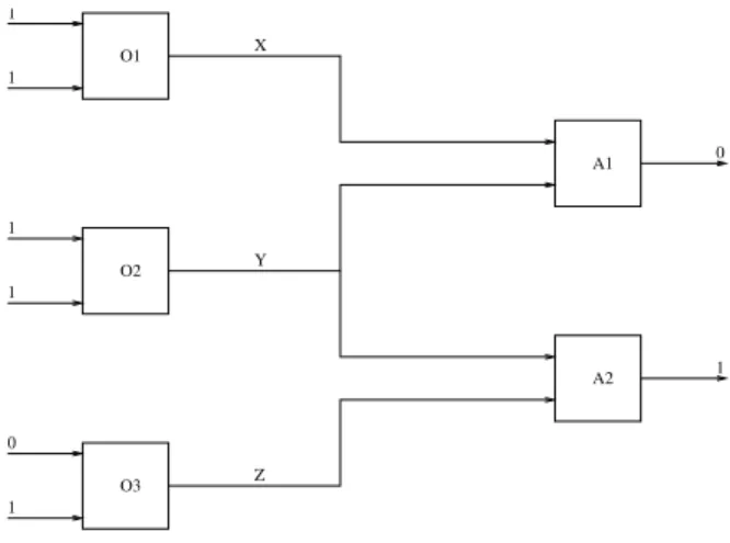
Figure 1: Topology of the boolean polybox The topology of the polybox is represented in figure 1. O1, O2, O3, A1, A2 are the components of the
sys-tem. O1, O2, O3are OR gates and A1, A2 are AND gates.
X, Y, Z are non-observable variables; each of those can take values in{0, 1}. mO1, mO2, mO3, mA1, mA2are mode variables associated to the components; each of those can take values in {G, B} (G for Good and B for Bad). A set of constraints link mode variables, observable and non-observable variables. When the non-observable variable values are provided, one can always instantiate observable vari-ables rather than keeping them in the model. This is why there are no observable variables in the polybox constraint model below.
For sake of clarity we use a constraint language which explicitly describes assignments of values to variables (we could have written the constraints in pure propositional logic). The constraints for the polybox are :
• (mO1 = G) =⇒ (X = (1 ∨ 1)) • (mO2 = G) =⇒ (Y = (1 ∨ 1)) • (mO3 = G) =⇒ (Z = (1 ∨ 0)) • (mA1 = G) =⇒ (0 = (X ∧ Y )) • (mA2 = G) =⇒ (1 = (Y ∧ Z))
These constraints can also be represented in extension be-cause, in this example, the domains of all the involved vari-ables are finite. For instance, the first constraint can be rewritten :{(O1, X), {(G, 1), (B, 0), (B, 1)}}.
Finally, the diagnosis problem of the polybox in the OCSP framework is :
• decision variables : {mO1, mO2, mO3, mA1, mA2}. Each associated domain is{G, B},
• non-decision variables : {X, Y, Z}. Each associated do-main is{0, 1},
• constraints are those described above. • cost function is g(mCi = vi) =
Q
jPj(mCi). Cost rep-resents the candidate probability. The component mode probabilities Pj(mCi) are combined with multiplication because faults on different components are assumed to be independent.
The associated constraint hypergraph is represented in fig-ure 2. O2 O3 A1 A2 O1 X Y Z
Figure 2: Constraint hypergraph of the boolean polybox
Hierarchical diagnosis and abstraction
Hierarchical diagnosis reasoning
Hierarchical diagnosis reasoning consists of solving a diag-nosis problem using an ordered list of diagdiag-nosis problems. Generally, this is initiated by a diagnosis problem P0 and
builds up to a more abstract diagnosis problem P1.
Itera-tively, one can build an ordered list of n diagnosis problems. Solving these problems is commonly achieved in a top-down fashion. First, the most abstract problem Pn−1 is solved.
Then (or at the same time), knowledge of solutions and non-solutions of Pn−1is used (through abstraction) to prune the
search space of the problem Pn−2. By iterating, one can
solve the original diagnosis problem P0. Results from
solv-ing problem Pkcan be useful for solving problem Pk−1in
different ways. It depends on the kind of abstraction which has been used to build problem Pk.
Abstraction concepts
In this section, different views of abstractions are described, each being more or less appropriate to exhibit properties in-teresting for diagnosis.
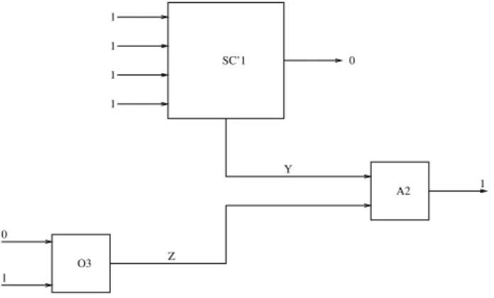
Topological view of abstractions (mapping of compo-nents) The topological view of abstractions relies on a component-centered representation. Graphically, as shown in figure 3, components are represented by nodes and la-beled by their name. The links between components are rep-resented by arcs (direction is chosen according to causality). Each arc is labeled by a value (observable variable) or the name of a non obervable variable. Some abstractions inter-pret naturally according to the topological view but others cannot be represented in this way. When such a representa-tion exists, topological views of the concrete model and of the abstract model are those giving the best intuition of the abstraction. SC’1 A2 O3 0 1 1 Z 0 1 1 1 1 Y
Figure 3: Topology of the abstract boolean polybox. Example In the polybox example, let us consider a simple structural abstraction (a special case of abstractions) which consists of aggregating for instance the components O1, O2
and A1 in one supercomponent SC1′. The topology of the
abstract polybox is represented in figure 3. But to com-pletely define this abstraction, the mapping between possible values of (mO1, mO2, mA1) and mSC1′ must be specified. As an example, a natural mode value mapping is :
• when (mO1 = G, mO2 = G, mA1 = G), then mSC′
1 = G, • mSC′
1 = B in other cases.
The topological view cannot capture all the abstraction information because the mode value mapping does not ex-plicitely appear.
This mode value mapping is represented in figure 4 and corresponds to the projection on D(mO1) × D(mO2) × D(mA1) → D(mSC′1) of an interpretation mapping as de-fined in (Nayak & Levy 1995). We can build any value map-ping among the28
possible mappings defined on D(mO1)× D(mO2) × D(mA1) → D(mSC′1).
It may be as well the case that mode variables can take more than two values. Some mappings can be more efficient than others, that is discussed in the fourth section. More general kinds of relations than mappings have been deeply described in (Lecoutre et al. 2006) but here, just mappings are considered.
m_SC’1 G G G G G G G G B B B B G G G G B B B B B B B B G B m_A1 m_O2 m_O1
Figure 4: A simple value mapping defined on D(mO1) × D(mO2) × D(mA1) → D(mSC′1).
Limits of the topological view In the last example, one can see that structural abstraction can naturally be defined by two choices :
• aggregation of variables (topological view), • aggregation of mode value tuples.
However, let us also notice that if we first choose an ag-gregation of mode value tuples, it implies an agag-gregation of variables; but the converse does not hold. This remark shows us that criteria for choosing good abstractions, even if it is in the structural abstraction case, can be more easily found by looking directly at the aggregation of mode value tuples (and not at the topological view). This leads us towards a new view of abstractions which corresponds to the search space view.
Search space view (mapping of states) The search space of a diagnosis problem is the set of possible complete as-signments to mode variables.
An extended mode value mapping (Lecoutre et al. 2006) (Nayak & Levy 1995) associates concrete states to abstract states. This extended mode value mapping can be found ex-tending a mode value mapping to all mode variables. The extended mapping, because its domain spawns on the whole search space, permits to evaluate the number of steps needed by a hierarchical diagnosis algorithm to solve a diagnosis problem. Given that the mode value mapping is gener-ally a surjective mapping (as in the polybox example), the extended mode value mapping is also surjective. Conse-quently, for each state of the abstract search space, the set of concrete states that correspond to it can be found thanks to the preimage of the extended mapping. The number of el-ements in this set is called the branching factor of an abstract state. Let us remind to the reader that the preimage of a sub-set B of the codomain Y under a function f is the subsub-set of the domain X defined by f−1(B) = {x ∈ X|f (x) ∈ B}.
The preimage exists even if the mapping is not bijective. The search space view is difficult to represent by a scheme when the number of components is high because the number of concrete states is exponential in the number of
compo-nents. In this paper, it is exactly2nstates for n components.
In our polybox example, the25
concrete states are abstracted into23
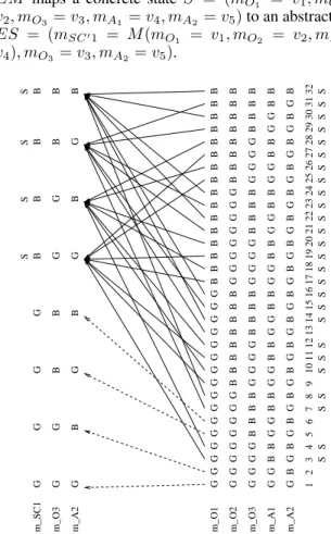
abstract states by the extended mapping. The latter that we note EM can be found given the mode value map-ping M represented in figure 4 in the following manner : • the domain of EM is D(mO1) × D(mO2) × D(mO3) ×
D(mA1)×D(mA2) → D(mSC′1)×D(mO3)×D(mA2), • EM maps a concrete state S = (mO1 = v1, mO2 = v2, mO3 = v3, mA1 = v4, mA2 = v5) to an abstract state ES = (mSC′1 = M (mO1 = v1, mO2 = v2, mA1 = v4), mO3 = v3, mA2 = v5).
G
m_O1 m_O2 m_O3 m_A1 m_A2
G G G G G G G G G G G G G G G G B B B B B B B B B B B B B B B B G G G G G G G G B B B B B B B B G G G G G G G G B B B B B B B B G G G G B B B B G G G G B B B B G G G G B B B B G G G G B B B B G G G G G G G G G G B B B B B B B B B B B B B B B B G G G G G G G G G G G G G G G G G G G G G G B B B B B B B B B B B B B B B B 1 2 3 4 5 6 7 8 9 10 11 12 13 14 15 16 17 18 19 20 21 22 23 24 25 26 27 28 29 30 31 32 S S S S S S S S S S S S S S S S S S S S S S S S S S m_SC1 m_O3 m_A2 G G G G B B B B S S S S G G G G G G B B B B B B B B G
Figure 5: The extended mapping for a structural abstraction of the polybox.
The extended mode value mapping EM is represented in figure 5. Each arrow represents a mapping from a concrete state to an abstract state. The symbol S denotes a state which is solution. One can see that there are 4 solutions to the abstract problem and 26 solutions to the concrete problem. Constraint view (mapping of constraints) The con-straint view of an abstraction is established by the concon-straint hypergraphs of the concrete and abstract OCSP’s.
The constraints of the concrete problem are abstracted into other constraints. In the example of the polybox, con-straints 1, 2 and 4 are merged into one constraint :(mSC′
1= G) =⇒ ((X = (1 ∨ 1)) ∧ (Y = (1 ∨ 1)) ∧ (0 = (X ∧ Y ))). Constraints 3 and 5 are preserved.
The search space view and the constraint view correspond to semantic and syntactic abstractions as defined in (Nayak & Levy 1995), respectively.
Influence of abstractions on computational
complexity
The word “best” in “best abstraction” is used for minimal computational temporal complexity, in other words for the minimum number of steps to solve the diagnosis problem. For this analysis, we consider that abstract diagnosis prob-lem(s) are precomputed, so we do not take into account the temporal computational complexity of constructing a hier-archical model of the system to be diagnosed (which is a reasonable hypothesis in the case of on-line state-tracking applications).
The analysis proceeds as follows : firstly, the set of so-lutions (hence the set of non soso-lutions) is supposed to be known. This permits us to give criteria of “good” abstrac-tions in the space search view; secondly, these criteria are interpreted in the topological and constraint views to deter-mine how they can be used to precompute “good” abstrac-tions that are garantied to be efficient.
Analysis in the search space view
Among all possible abstractions, two general kinds have been identified in the litterature (Nayak & Levy 1995) (Chit-taro & Ranon 2004) (Lecoutre et al. 2006). :
• Concrete Solution Increasing (CSI), • Concrete Solution Decreasing (CSD).
Definition 4 (CSI abstraction) An abstraction is CSI iff for
all concrete states which are solutions of the concrete prob-lem, their corresponding abstract state (w.r.t extended mode value mapping) is solution of the abstract problem.
From this definition, one can trivially deduce the follow-ing proposition :
Theorem 1 Consider a CSI abstraction, then if an abstract
state is shown not to be solution, then all its correponding concrete states are not solutions.
For example, the structural abstraction of the polybox mentioned above is CSI, one can verify it in figure 5. Definition 5 (CSD abstraction) An abstraction is CSD iff
for all concrete states which are not solutions of the concrete problem, their corresponding abstract state (w.r.t extended mode value mapping) is not solution of the abstract problem.
From this definition, one can trivially deduce the follow-ing proposition :
Theorem 2 Consider a CSD abstraction, then if an abstract
state is shown to be solution, then all its correponding con-crete states are solutions.
A general and simple hierarchical diagnosis algorithm be-gins from the most abstract problem, generates and tests all the states of a level n in the abstraction hierarchy, then goes down to the level n− 1, and iteratively, the algorithm fin-ishes to test all the concrete states of the level0 to give the solutions of the concrete problem.
In this paper, we consider two levels in the abstraction hierarchy but the results can be extended to more than two levels.
Let us recall to the reader that without abstraction, with a simple-minded diagnosis algorithm which just generates and tests states, the temporal computational complexity is O(n) where n is the number of states of the diagnosis problem, i.e. exponential in the number of components.
Consequently, the temporal computational complexity of the hierachical diagnosis algorithm described above depends on two factors :
• the number of abstract states, • the number of concrete states.
The number of concrete states cannot be changed. An ideal abstraction would consist of two abstract states a and b. a maps all the states which are solutions and b maps all the states which are not. Let us notice that the ideal abstraction we propose is CSI and CSD. So an abstract solution is suffi-cient to represent all the solutions of the concrete problem; and a non solution abstract state rules out all the non solu-tion concrete states. Consequently, from the CSI and CSD propositions, one can deduce the following proposition : Theorem 3 An abstraction that is CSI and CSD reduces the
complexity of the diagnosis problem to O(n′) where n′is the
number of abstract states. The ideal CSI and CSD abstrac-tion has two abstract states.
But this ideal abstraction cannot be easily built for two reason :
• which states are solutions and which are not is not known in advance,
• constraints associated to the abstract states may not exist. Refering to the first issue, solutions are supposed to be known (for the analysis) to target which abstractions can easily capture solutions and non solutions. We tackle the second issue using the constraint space view to exhibit ab-stract constraints which can be easily built.
It appears that the ideal abstraction does not exist in the general case. However one can capture all the solutions and non solutions of a problem using several abstractions of the same problem.
Example
For the polybox example, there are 32 states and, among them, 26 solutions. The diagnosis community is used to represent the 26 solutions by 3 minimal diagnoses : {O1}, {A1}, {O2, A2}. These minimal diagnoses represent
16, 13 and 8 solution states, respectively. Some states are represented by several minimal diagnoses. Non solution states can be captured by minimal conflicts. Minimal con-flicts{O1, O2, A1} and {O1, A1, A2} each captures 4 non
solutions.
The ideal abstraction of the polybox example maps the 26 solutions to one abstract state a and the 6 non solutions to another abstract state b. But with such a partition of the search space, building abstract constraints means solving di-agnosis problem. However, given that we want to build hi-erarchical model for all possible set of inputs, this approach is not feasible. One may however notice that using abstract states corresponding to minimal potential conflicts (Cordier
et al. 2004), we can build a relatively efficient hierarchical model for all sets of inputs. All non solutions are captured and ruled out in an efficient way. This idea is developped in the next subection.
Using constraints to find “best” abstractions
We can relax the ideal abstraction requirement using sev-eral “two abstract states-based” abstractions to capture the whole search space. One needs, for each abstraction, one abstract state which can represent the highest number of non solutions and another abstract state to represent the highest number of solutions.
To choose these states, the topological and constraint views of abstractions are used. Choosing abstractions in the search space view may lead to non existant abstract CSPs, i.e. for which one cannot find the corresponding variables and constraints.
To represent a maximal number of states, one has two main choices :
• aggregating variables and mode values as described in the topological section,
• removing variables and/or values.
In the constraints view, aggregating variables corresponds to merging constraints and removing variables corresponds to removing constraints. The first option exactly corre-sponds to structural abstraction and one can see in the poly-box example that with natural mappings, abstraction is CSI but does not permit to rule out a lot of non solution states in one test. For the second option, removing n variables per-mits one to represent2n states. So, one has to remove the
highest number of variables while keeping the constraints decidable. Removing variables means removing their asso-ciated constraints. Consequently, one must find the smallest set of constraints which remain decidable. These sets are hence just overdeterminated, i.e. they involve n equations for n− 1 unknowns, and they are well-known in the diag-nosis field as corresponding to minimal potential conflicts (Pulido & Alonso 2002) (Cordier et al. 2004).
When the test on a given OBS of one such just overdeter-minated constraint set does not pass, the conjunction of as-signments to G of the involved mode variables is a minimal conflict. The case in which at least one variable is assigned to B does not help for finding solutions since the constraints are always satisfied. It is easy to show that when using a minimal potential conflict to construct an abstraction, this abstraction is CSI but not CSD. It is also known that all mini-mal potential conflicts capture all concrete non solutions. So checking all the abstract states built this way garanties to rule out all the non solution states. However, one abstraction per minimal potential conflict is necessary since one concrete state may correspond to more than one minimal potential conflict. Indeed, we have restricted our analysis to map-pings between concrete states and abstract states. With gen-eral relations, we conjecture that one abstraction can contain all minimal potential conflicts but in this case, one concrete state may have more than one image.
Conclusion and future work
Hierarchical diagnosis efficiency strongly depends on the choice of the abstractions used to build a hierarchical model of the system. For analysing the influence of this choice, three complementary views of abstractions have been de-fined : the topological view, the search space view and the constraint view. In the case in which abstractions are built removing variables or contraints, we argue that most effi-cient abstractions are obtained from minimal potential con-flicts because they rule out all non solution states.
But finding efficient abstractions has a cost. For instance, determining minimal potential conflicts is known to be of exponential complexity. So our future work will focus on defining an efficiency measure for an abstraction that takes in account not only the computational gain on the hierarchi-cal model but also the cost of finding the model. In par-ticular, we will pay much attention to structural abstraction because it is generally cheap; and we will consider building a bridge between structural abstractions and other types of abstractions (like conflict-based) that all together may boost the diagnosis resolution process efficiency.
References
Chittaro, L., and Ranon, R. 2004. Hierarchical model-based diagnosis model-based on structural abstraction. Artif.
In-tell.155(1-2):147–182.
Cordier, M. O.; Dague, P.; Levy, F.; Montmain, J.; Staroswiecki, M.; and Trav´e-Massuy`es, L. 2004. Con-flicts versus analytical redundancy relations : a compara-tive analysis of the model-based diagnosis approach from the artificial intelligence and automatic control perspec-tives. IEEE Transactions on Systems, Man and
Cybernet-ics.34(5):2163–2177.
Hamscher, W.; Console, L.; and de Kleer, J. 1992.
Read-ings in model-based diagnosis. Morgan Kaufmann. Lecoutre, C.; Merchez, S.; Boussemart, F.; and Gr´egoire, E. 2006. A csp abstraction framework. Revue d’intelligence artificielle20(1):31–62.
Nayak, P., and Levy, A. 1995. A semantic theory of ab-stractions. In Mellish, C., ed., Proceedings of the
Four-teenth International Joint Conference on Artificial Intelli-gence, 196–203. San Francisco: Morgan Kaufmann. Pulido, B., and Alonso, C. 2002. Possible conflicts, arrs, and conflicts. Proceedings of the Thirteenth International
Workshop on Principles of Diagnosis (DX 02).
Torta, G., and Torasso, P. 2006. Qualitative domain ab-stractions for time-varying systems: an approach based on reusable abstraction fragments. In Proc 17th Workshop on
Principle of Diagnosis (DX 06).
Williams, B. C., and Ragno, R. J. 2003. Conflict-directed a* and its role in model-based embedded systems. Journal