Calibrating activity-based travel demand model system via microsimulation

Calibrating Activity-based Travel Demand Model

System via Microsimulation

by

Siyu Chen

B.S., University of California, Berkeley (2017)

Submitted to the Department of Civil and Environmental Engineering

in partial fulfillment of the requirements for the degree of

Master of Science in Transportation

at the

MASSACHUSETTS INSTITUTE OF TECHNOLOGY

June 2019

Massachusetts Institute of Technology 2019. All rights reserved.

Author

...

Signature redacted...

Department of Civil and Environmental Engineering

May 17, 2019

Signature redacted

C ertified by

... ..

...

Moshe E. Ben-Akiva

Edmund K. Turner Professor of Civil and Environmental Engineering

Thesis Supervisor

i

fl'1i.

Signature redacted

Accepted by

...

Seau

epf

/ 1

1

He diNepf

Donald and Martha Harleman Professor of Civil and Enviro

ental

MASSACHUSETTS INSTITUTE

_Engineering

OF TECHNOLOGY >

0

Chair, Graduate Program Committee

JUL 1

02019

Calibrating Activity-based Travel Demand Model System via

Microsimulation

by

Siyu Chen

Submitted to the Department of Civil and Environmental Engineering on May 17, 2019, in partial fulfillment of the

requirements for the degree of Master of Science in Transportation

Abstract

This thesis addresses the problem of calibrating activity-based travel demand model systems. After estimation, it is common practice to use aggregate measurements to calibrate the estimated model system's parameters. However, calibration of activity-based model systems has received much less attention. Existing calibration ap-proaches are myopic heuristics in the sense that they do not consider inter-dependency among choice-models and do not have a systematic way to adjust model parameters. Also, other simulation-based approaches do not perform well in large-scale applica-tions. In this thesis, we focus on utility-maximizing nested logit activity-based model systems and calibrating count based aggregate statistics like OD flows, mode shares, activity shares and so on. We formulate the calibration problem as a simulation-based optimization problem and propose a stochastic gradient-based solution procedure to solve it.

The solution procedure relies on microsimulation to calculate expected aggregate statistics of interest to the calibration problem. Additionally, we derive approximate analytical expressions for the gradient of the objective function -that are evaluated through microsimulation on mini-batches of the population. The proposed solution procedure is sensitive to the fundamental structure of the activity-based model sys-tem and is non-myopic in considering the dependencies across its model components. Finally, we show -through a real-world application- that the proposed solution procedure outperforms other state-of-the-art purely simulation-based optimization approaches in terms of computational efficiency, stability, and convergence. We also compare various gradient-based solution algorithms to determine the best algorithm to update the parameters. This work has the potential to facilitate wider and easier application of activity-based model systems.

Thesis Supervisor: Moshe E. Ben-Akiva

Acknowledgments

First and foremost, I would like to express my deepest gratitude to my research advisor and thesis supervisor Professor Moshe Ben-Akiva for his patient guidance and useful critiques. Not only he provided me invaluable suggestions on several research projects, but also he set very high standards for me and pushed me to do better.

I would also like to extend my deepest gratitude to Dr. A. Arun Prakash. He played a decisive role in coming up this research idea with me. This thesis would not have been possible without his patient support and numerous advice. Apart from this thesis, he constantly provided invaluable insight into other research projects I involved with.

I must also thank Professor Carlos Lima De Azevedo, Dr. Jimi Oke, and Dr. Ravi Seshadri for their great amount of assistance on research projects.

I also had great pleasure of taking multiple useful courses with amazing professors at MIT. Their knowledge, expertise and wisdom are valuable to me.

I am very grateful to my colleagues: Youssef Medhat Aboutaleb, Mazen Danaf and Yifei Xie. I feel fortunate to study and work with them. I got inspired by them from time to time.

Last but not least, I am deeply indebted to my parents for their endless love and continuous support.

Contents

1 Introduction 13

1.1 Activity-based models . . . . 14

1.2 Thesis motivation and objective . . . . 15

1.3 T hesis outline . . . . 16

2 Background 19 2.1 Calibration of trip-based models . . . . 19

2.2 Calibration of activity-based models . . . . 21

2.3 Sum m ary . . . . 25

3 Methodology 27 3.1 O verview . . . . 27

3.2 Problem Definition . . . . 28

3.2.1 Generic ABMs structure . . . . 28

3.2.2 Problem formulation . . . . 30

3.2.3 Evaluating the objective function via microsimulation . . . . . 32

3.3 Solution procedure . . . . 35

3.3.1 Description of the solution procedure . . . . 35

3.3.2 Flow of gradient computation . . . . 37

3.3.3 Derivation of the gradient of the objective function with respect to choice-niodel specific coefficients . . . . 38

4 Illustrative example 51

4.1 Overview . . . . 51

4.2 Solution procedure application . . . . 53

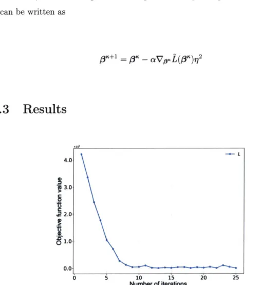
4.3 Results . . . . 56 5 Case Study 59 5.1 Overview . . . . 59 5.1.1 Day Activity-Schedule . . . . 60 5.1.2 Simulation set up . . . . 62 5.1.3 Problem formulation . . . . 62 5.2 Application . . . . 67

5.2.1 Numerical gradient check . . . . 67

5.2.2 SPSA . . . . 68

5.2.3 Stepsize tuning . . . . 70

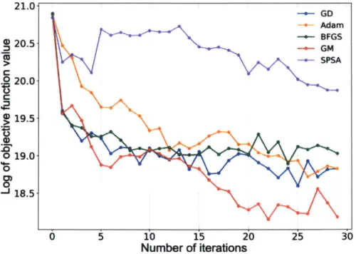
5.2.4 Performance comparisons . . . . 71

List of Figures

3-1 A BM s graph . . . . 29

3-2 Flow of gradient computation . . . . 39

4-1 Illustrative example . . . . 52

4-2 Illustrative example objective value plot . . . . 56

5-1 DAS ABMs structure . . . . 61

5-2 Convergence comparison . . . . 72

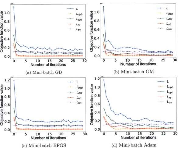
5-3 Four algorithms' objective function component values plots . . . . 73

List of Tables

3.1 Table of important notation . . . . 28

4.1 Illustrative example result table . . . . 58

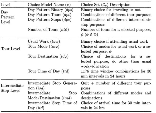
5.1 DAS model system . . . . 62

Chapter 1

Introduction

Travel models are created to help managers, planners and directors make informed decisions. They produce quantitative information about travel demand and trans-portation system performance. There are various forms of travel models developed with different modeling assumptions and purposes. Using person-trips as the unit of analysis, trip-based models, developed in the 1950s, are widely used in practice. However, trip-based models suffer from several major limitations. First, trip-based models are not behaviorally realistic. They model demand for trip making rather than for activities. Second, because trip-based models are based on person-trips, they do not capture any dependency among household members. Third, they assume that individuals within the same group share the same characteristics, which causes demographic aggregation errors. Also, they suffer from spatial and temporal aggre-gation errors because they assume all households in a zone are treated as identical and only differentiate between peak and off-peak periods. Fourth, they cannot model induced travel because each person-trip is independent. Because of aforementioned drawbacks, limited types of policies can be analyzed and activity-based models are developed.

1.1

Activity-based models

Based on the principle that travel demand derives from activities, activity-based models model individual's behaviors sequentially in a continuous domain of time and space. Rasouli and Timmermans [1] identified three activity-based modeling approaches: 1). constraints-based models, 2). utility-maximizing models, and 3). computational process models. They are mainly different in terms of the way to model individual and household activity patterns.

Constraints-based models are able to identify feasible activity schedules under space and time constraints instead of directly predicting individual and household activity-travel patterns. However, they have several limitations, including the limited consideration on household accessibility instead of individual accessibility, the unre-alistic assumption of isotropic conditions [2], and lack mechanisms to deal with choice behavior under uncertainty. Regarding these limitations, some generalizations of the classic space-time prism are proposed to address them and are brought together in

[3].

On the other hand, utility-maximizing models utilize discrete choice models and other econometric models to maximize individual's utility in choosing among travel patterns. As an advanced model applied widely in practice, the day activity schedule (DAS) model system [4, 5, 6, 7, 8, 9] is a nested logit model system consisting of several nests to model travel choice as a multidimensional choice with shared unobserved elements. The topmost choice is activity pattern choice, in which time of day, mode and destination for primary tour, time of day, mode and destination for secondary tour are modeled. Conditional on the activity pattern choice, lower levels include time-of-day, mode and destination choice for the primary tour, time-of-day, mode and destination choice for the secondary tours. However, it has coarse representation of schedule as combinations of discrete time periods. Apart from the DAS model, there are other activity-based models, like the Prism-Constrained Activity Travel Simulator (PCATS) [10], the Comprehensive Econometric Micro-simulator for Daily Activity-travel Patterns (CEMDAP) [11], and the Comprehensive Utility-based System of

Travel Options Modelling (CUSTOM)[12].

More recently, computational process models are created to relax the strict and behaviorally unrealistic assumption of utility-maximizing behavior. The most com-prehensive one is Albatross [13], which controls the scheduling processes in terms of a sequence of 27 steps. However, such scheduling process is based on a priori assump-tions of the researchers. Some other applicaassump-tions are SCHEDULER [14], AMOS [15] and ADAPTS [16].

1.2

Thesis motivation and objective

As a result of research in various modeling aspects over the past years, Activity-Based Model systems (ABMs) have become a part of integrated travel demand model systems. However, the fundamental task of calibrating ABMs has received limited attention in literature. In this light, this thesis presents a systematic ap-proach to calibrate ABMs that explicitly considers the complex interactions among its components.

The motivation for this study is threefold. First, although ABMs is a powerful and widely accepted modeling framework, there are limited studies on their calibra-tion. Efficiently calibrating these model systems is crucial for their wider and easier application. Second, the existing calibration approaches for ABMs are predominantly myopic heuristics that overlook inter-dependency among choice-models and can re-sult in ill-formed model systems -especially in complex ABMs. Third, relying on "black box" -purely simulation-based- approaches to calibrate ABMs have not been successful in large-scale applications.

In light of the aforementioned motivations, the objectives of this thesis are as follows:

1. To propose a generic mathematical formulation of the ABM calibration problem.

2. To propose an efficient solution procedure, adopting microsimulation and struc-tural relationships within the ABMs.

3. To apply and test the proposed formulation and solution procedure on an ex-isting ABM.

This study contributes to the existing literature in following aspects. First we formulate the ABM calibration problem as a simulation-based optimization problem. Second, for nested logit activity-based models, we derive the expressions for unbiased estimators of the simulated aggregate statistics of interest which are used in the ob-jective function of the calibration problem and can be computed via microsimulation. Third, using the proposed analytical expressions of the objective function we derive an unbiased estimator of the gradient of the objective function -with respect to any parameter of interest in the DAS model system- through microsimulation. Fourth, this proposed generic approach is able to get both objective function and its gradient in a single run of the microsimulation. It explicitly considers the structure of the ABMs to accurately and efficiently calculate the gradient of the objective function without the need to rely on commonly used black-box approaches. Fifth, we propose a stochastic gradient-based approach that uses a sample of the population to iteratively solve the formulated problem. Finally, we demonstrate the correctness and efficiency of the procedure through a real-world application and test various gradient-based solution algorithms. Comparison with the existing simulation based state-of-the-art algorithms -simultaneous perturbation stochastic approximation (SPSA)[17]-showed that the proposed algorithm is computationally efficient, more stable, and results in faster convergence.

1.3

Thesis outline

Chapter 2 examines past travel demand model calibration efforts. Following past development, Chapter 3 formulates the calibration problem as a simulation-based optimization problem and proposes a gradient-based solution procedure to solve the optimization problem. In addition, it also reports derivations of analytical gradient expressions. Chapter 4 contains a illustrative example for better understanding of the solution procedure. Chapter 5 presents the results from experiments done on a

prototype city to demonstrate the efficacy of the calibration approach. The conclu-sions drawn from the research are reported in Chapter 6, along with future research work.

Chapter 2

Background

Transportation Model Systems have become more complex as a result of readily available computational resources and the need to more realistically model activity-travel planning. Further, various simulation systems are being developed as tools to facilitate analysis and decision-making by researchers, practitioners, and policy-makers [18, 19, 20]. It is increasingly being recognized that calibration and validation of these model systems, specifically the activity-based models, is one of the key aspects that needs to be addressed for a wider and more reliable application of the modeling tools. Yet, very little attention has been devoted to the development and application of robust techniques for calibrating the demand-side parameters of activity-based model systems.

2.1

Calibration of trip-based models

Calibration of traditional trip-based models has a long history and includes ap-proaches that are both manual and algorithmic. The manual approaches involve estimating and constructing of the model system and then adjusting individual mod-els in it to better match the observed statistics. Some of the techniques include (i) adjusting zonal scaling factors, (ii) introducing OD K-factors, (iii) changing alterna-tive specific constant of the mode choice-models. The zonal scaling factors are used for some specific zones to adjust the trips generation and attraction rates [21].

Simi-larly, OD K-factors are constants that are added to specific origin-destination pairs in the destination choice-models (or trip generation models) to make OD flows of mod-els closer to the observed statistics [22]. Finally, the alternative specific constants of the modes are changed such that mode-shares from the model match the observed statistics

[23].

Algorithmic approaches to calibrate trip-based models have been predominantly focused on estimating OD matrix. Three modeling approaches are postulated in [241: traffic modeling based approaches, statistical inference approaches and gradient based solution techniques. As an example, [251 formulated the problem as an analytical op-timization problem where the observations were the sensor counts. Recently, the OD estimation problems have been formulated as simulation-based optimization prob-lems and solved using stochastic algorithms [26, 27, 281. The trip-based models are considered in the OD estimation problem through a seed matrix that is part of the objective function. [26] concludes that simultaneous perturbation stochastic approx-imation (SPSA) performs well in real word applications in terms of solution quality and computational efficiency compared to other simulation optimization algorithms like Box-Complex, SNOBFIT, and finite difference stochastic approximation (FDSA).

Both FDSA and SPSA are stochastic approximation (SA) algorithms. With model parameters of interest denoted as 3 and formulated objective function denoted as

L(/3), both algorithms use approximate gradient of objective function denoted as

VaL'(,3) to update model parameters. The update rule at iteration r, can be written as:

1

=3K

- a"VOL'()3K)

(2.1)

where a' represents the step size at iteration r,, which becomes smaller as K increases.

However, FDSA approximates the gradient by perturbing each parameter of 0 in both plus and minus direction separately and takes 21,31 runs to approximate while

SPSA efficiently estimates the gradient by perturbing all parameters in 3 simultane-ously. Thus the approximation of gradient only needs two function evaluations instead of 211 function evaluations in FD scheme. In terms of convergence performance, [171 argues that SPSA performs as good as FDSA while has 1/31-fold simulation saving. In this study, we compare our proposed solution procedure with SPSA and more detail about SPSA algorithm is in section 5.2.

However, the performance of SPSA suffers from gradient approximation error when it is applied to a large-scale system with sparse correlations between parameters and measurements. [27, 28] propose Weighted SPSA (W-SPSA) to overcome this limitation by relying on a weight matrix, which represents the appropriate correlation structure. However, generating the essential ingredient -weight matrix- is not systematic, which considerably limits the applicability of the algorithm.

[29, 30] also propose a computationally efficient metamodel simulation-based op-timization approach, which embeds within the simulation-based opop-timization algo-rithm information from an analytical yet differentiable and tractable network model. In addition, online estimation of OD matrix for real-time applications has also gained attention [31] with recent work on the problem scalability [32, 33].

2.2

Calibration of activity-based models

Calibration of activity-based model systems has received much less attention in the literature although they are increasingly applied in practice [34, 35, 36, 20]. ABMs also get questioned by many practitioners because it is in many aspects easier to adjust four-step models to fit base level traffic counts exactly [37]. The prevailing practice, which is similar to that of the trip-based models, is to calibrate individual models to better match the observed statistics [38]. Researchers and practitioners have been using top-down model-specific sequential methods, since adjustments to upper level models will tend to have a higher impact on lower level models than vice-versa. [38], for example, calibrated sequentially from the top to the bottom of the DaySim model hierarchy: longer term person and household choices, single

day-long activity pattern choices, tour-level choices, and trip-level choices. As the number of parameters in each level can be quite significant, such calibration generally focuses on the adjustment of alternative specific constants, which tend to capture the effects of variables ignored in the estimation phase [391. Such adjustment procedure has also been recently proposed when transferring an existing model system and re-calibrating it with local data to a new region

140].

In similar settings, to minimize the burden of the manual iterative procedure at each model level, some researchers and practitioners adopt an incremental alternative-specific constant adjustment method using dampening factors [41, 231. When an aggregate measurement for a given choice dimension is available in terms of shares (e.g.: mode share, activity type shares, etc) constants are updated at each iteration as follows:

=

+~~2

DF,,i

*

1n

( j

where r, is the iteration index, 3g i is the alternative specific constant coefficient p in the utility expression of alternative i in a choice-model 7 to be calibrated, Ari is the observed share of alternative i, S1i is the estimated share of alternative i at iteration K. The DF is the dampening factor usually set between 0.10 to 0.75 which helps eliminating the oscillating pattern between iterations of the calibration procedure.

It is common practice to normalize the above adjustments by setting one alter-native as a baseline and subtracting its adjustment from all the alteralter-natives. The steps described above are repeated till the predicted and the observed distributions are satisfactory close. This state-of-the-practice method is highly limited in the cov-ered degrees of freedom and the considcov-ered interactions between the different model system components, thus often forcing modellers to iteratively revisit the estimation phase and slows down the calibration process [421.

[43] proposed that the activity-based models can be calibrated to external OD flow information derived from traffic counts in an indirect approach or direct approach. The indirect approach tries to analyze traffic counts, for example, identify effects of holidays and weather effects, and incorporate findings into the model components

of activity-based models. However, this indirect approach requires changes of model specifications and specifically works for calibrating traffic counts. In addition, the authors do not discuss the influence of such indirect approaches on other models' results.

The direct approach proposed by [431 to fine-tune activity-based models' param-eters can be done at four different levels: the data level, the model level, the OD-matrix level and the assignment level. As the data level, the calibration approach attributes weights to the different agents and generate new activities using updated data. However, the weighting procedure can become very computationally intensive as the number of agents increases. In addition, we cannot use activity-based models to do predictions because models' parameters are not adjusted according to observed statistics.

At the model level, without considering route choice and mode choice, they pro-posed a heuristic approach to adjust only destination choice-models in the model system and demonstrated the approach on a small 10-zone network. Although they recognized the need to calibrate the complete ABMs considering inter-dependency and admitted the complexity would increase significantly, they did not discuss any solution for such situation.

At the OD-matrix level, we have briefly mentioned common approaches in previous section. The problem of applying OD-matrix estimation approaches on calibration is that forecasting future year matrices needs extra attention. The adjustments per-formed on the OD-matrix in the base year need to be somehow reflected in forecasted matrices. Absolute difference or percentage of change between simulated OD matrices and adjusted matrices for the base year can be applied to future matrices. Another problem is that OD-matrix estimation approaches cannot be used to calibrate other aggregate statistics like certain activity-purpose share or mode share.

At the traffic assignment level, the way of assigning OD flows to the network plays a important role in matching model-based traffic counts with the benchmark measures. However, calibration approaches at this level do not consider if other measures, like the number of individuals traveling, match or not. It also has the

similar prediction issues because model parameters do not adjust.

[441

elucidated the limitations of existing calibration approaches and proposed using Taguchi experimental design and ANOVA to improve the calibration process. They used Taguchi experimental design to identify the models/parameters that have impact on the outputs in a robust manner: ANOVA was applied to determine the effectiveness of models/parameters on the outputs of interest. However, the method-ology to adjust the parameters is a heuristic that relies on the outputs from running the simulation with different level of the parameters which might result in premature solutions and intractable number of simulation runs.

Researchers have stepped away of the direct modelling of all these complex inter-actions in activity-based model systems. Approaches mentioned in previous section like SPSA are applied to calibrate ABMs. In addition, [45 adopted an iterative black-box methodology for the calibration of POLARIS, assuming to only know the inputs and outputs of the entire modelling process. By using a meta-model of the model system surrogate, the authors evaluated and estimated the unknown relationship be-tween the simulated results and observed outputs at a given input set. A Gaussian Process over all potential functions representing this relationship was determined at each iterative step utilizing Bayesian estimation. Active learning methods are used for sample determination in the exploration phase. However, the authors still point out the computational intractability of the proposed process, as it resulted in long and costly simulations for a single experiment alone.

Fltterdd [46] presents an approach to calibrate both DTA simulators and disag-gregate demand models' parameters within a Bayesian framework at individual level. Relying on an agent-based dynamic traffic simulator, the analyst's prior knowledge is represented by the simulator and measurements are time dependent traffic counts. Then priori assumption about every individual's choice distribution is combined with available measurements' likelihood from simulator to form an estimated posterior choice distribution. The authors also show that the framework is capable of handling large scenarios [471. However, this calibration framework only limit to traffic counts

2.3

Summary

In summary, studies on calibration of models for demand generation in transportation model systems have focused primarily on trip-based models. Although, activity-based models are increasingly being adopted in practice, effectively calibrating them has been a challenge because it is complex and computationally intractable. This study tries to address this critical gap by proposing an optimization framework and algorithm to effectively calibrate activity-based model systems.

Chapter 3

Methodology

3.1

Overview

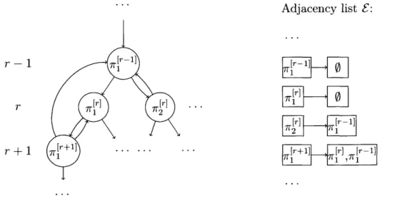
As discussed briefly earlier, the activity-based model system in this paper refers to utility-maximizing nested logit ABMs. In this chapter, we discuss calibrating count based simulated aggregate statistics acquired from simulating ABMs against actual aggregate statistics acquired from travel diary, transit on-board surveys, screenline and other counts. Section 3.2 first introduces a generic ABMs structure and then formulates calibration problem as an optimization problem to minimize the distance between simulated aggregate statistics and actual aggregate statistics. In addition, we propose to use expected simulated aggregate statistics from ABMs outputs as estimates of true simulated aggregate statistics to avoid dealing with uncertainties from activity generation and make objective function value deterministic for given choice-model coefficients. Then we derive simple analytical expressions of simulated aggregate statistics in the objective function that can be evaluated through microsim-ulation utilizing the structure of ABMs and closed form of logit choice-model's proba-bility expression. Following that, section 3.3 explains the complete solution procedure to solve the optimization problem and explains two important aspects of the solu-tion procedure -gradient computation and parameter update- in detail. Important notations are shown in table 3.1.

n Individual/agent' n JV Full set of individuals simulated (complete population) I -|Cardinality

II Set of all choice-models in the ABMs

Set of choice-models to calibrate in the ABMs, It c

i

7r _Choice-model 7r, 7r E H

X, Set of individuals on whom the choice-model

7r

will be run

77r Individual n's choices in upper level choice-models lead to current choice-model 7r

C, Choice set of choice-model

7r

1911 Expected number of individuals from ABMs choosing choice-model 7r's alternative i

Swi Estimated number of individuals from ABMs choosing choice-model 7r's alternative i

A,i Actual number of individuals choosing choice-model 7r's alternative i

X~ri Vector of individual n's characteristics and attributes of choice-model ir's alternative i Un, Individual n's utility of choice-model 7r's alternative i

V,,n Individual n's systematic utility of choice-model ir's alternative i

En Individual n's random utility

Vwn Individual n's systematic utility vector for choice-model ir P,(7ri) Individual n's probability of choosing choice-model 7r's alternative i

A,,,, Individual n's inclusive value/logsum term of choice-model 7r

#ai Coefficient' p of choice-model 7r's alternative i

00 Vector including apriori values of #ti, we want to calibrate

0 Vector including current values of #,i, we want to calibrate

a Step size used to update coefficients

Wiri Weight of choice-model 7r's component i in objective function

r; Number of mini-batches

a-(.) Sigmoid function

() Softmax function

f(-)

Microsimulation function

L(.) Objective function

Lr(-) Component of choice-model ir in objective function L

VOL(.) Gradients of objective function with respect to 8

Statistics or objective value associated with mini-batch

K Iteration number

Table 3.1: Table of important notation

awe use individual and agent interchangeably

bwe use coefficient and paramter interchangeably

3.2

Problem Definition

3.2.1

Generic ABMs structure

In this section, we define a graph G = (H, R, D) to present an Activity-Based Model

system. H is a set of nodes and each node, ir E H, represents a choice-model. R is

a set of ordered levels and each level contains at least one model 7r. A

choice-model

7r

located at level

r

is denoted as irgr] and upper level choice-models have smaller

level number. D is a set of directed edges, which represents inter-dependency among choice-models.

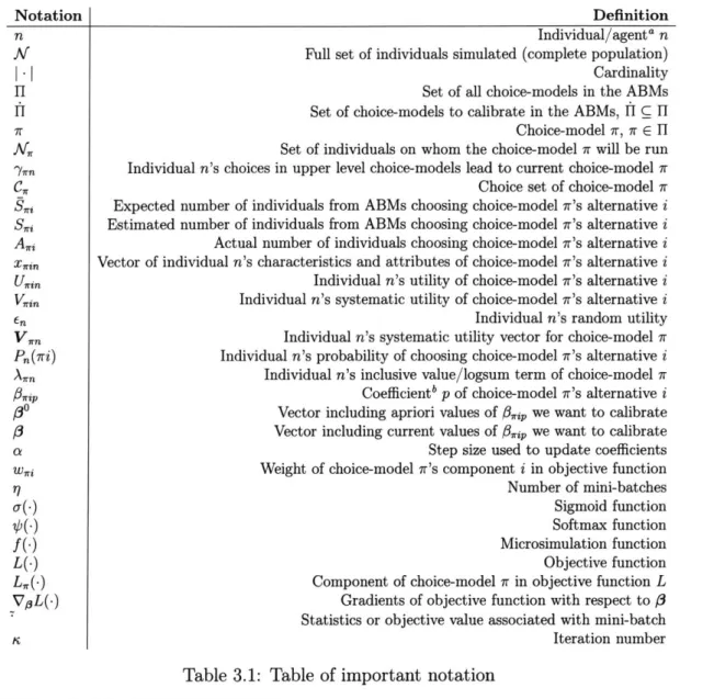
In addition, E is an adjacency list with size equal to the number of nodes, JrIi. An entry 9[7r] represents the list of upper level choice-models -above than choice-model 7r- dependent on the choice-model 7r through logsum term or inclusive value [481 of model 7r. Logsum term of lower level model makes upper level choice-models sensitive to important attributes that are measured directly only at the lower levels of the model.

Without loss of generality, we assume that any choice-model ir, located at level r as 74r1 in the given ABM system, except the root choice-model (r ' 1), is only directly

dependent on a choice-model 7

rq in one level above, 7rq This means that in the

ABMs graph G, there is an unique downward path from the root node to a lower level choice-model 7rj 1. In other words, there is only one possible choice combination

from the root choice-model leading to a lower level choice-model. Adjacency list E:

r~7 [0 r

r 4[ r

~A

] .. .. [r+1] [) r 1

Figure 3-1: A part of Activity-Based Model system graph G. Each circular node represents a choice-model 7r and each arrow represents the dependency of the end node on the start node. I={1 .r-1 , , [r] r [r+,= ,r-1, rr+1, }

,1 ) 1 2~ 1

A part of ABMs graph is shown in Figure 3 - 1. There are four choice-models located on three different levels as a part of a activity-based model system. The dependency shown in the figure includes the dependency of the lower level

choice-model on the upper level choice-choice-model. Also, it includes the dependency of the upper level choice-model on the lower level choice-model through logsum, which is represented by adjacency list E. For example, an entry E[7r j[+]] is a list of two elements: 7r] and 7rr-1, which represents that upper level choice-models 7r-] and

irj depend on the choice-model 7r+01 located on the lower level r

+

1. The following calibration problem formulation and solution procedure illustration are based on these four choice-models. However, they can easily be generalized to calibrate any set of choice-models within a ABM system as we show in section 3.2 and section 3.3.

3.2.2

Problem formulation

To calibrate this generic ABMs, we need the following two categories of variables: 1). actual observed aggregate statistics and 2). simulated aggregate statistics. In this study, we focus on calibrating count based aggregate statistics. The commonly avail-able count based aggregate statistics are the following: number of individuals travel-ing, number of individuals performing each activity, number of tours corresponding to each activity, number of tours/trips corresponding to each mode, and origin and destination flows at a zonal level. The first four statistics are generally obtained from survey data and expansion factors. The OD flows can generally be obtained from an existing planning model or from an OD estimation procedure performed on the network.

To formulate the problem, let 1 = {[r-,7r],7r,7r }1 I represent the set of

choice-models needed to be calibrated among all choice-models in the ABMs and let C, represent the set of alternatives in a choice-model -r. Further, let Si denote the estimated number of individuals choosing alternative i E C, in choice-model 7r, and ARi denote the actual number of alternative i E C, in choice-model 7r. Let fpi

represent the coefficients/parameters in the utility expression of alternative i E C, in choice-model 7r. The objective of calibration problem is to determine 3,'s -for the selected choice-models and their alternatives- such that the discrepancies between the simulated aggregate statistics and actual aggregate statistics are minimized. The vector including all 3's is denoted as 3. Coefficient p in Oi is denoted as Oi.

As we want to minimize the difference between Si and Ai for all choice-models

in f by updating 3 between its lower bound

/LB

and upper bound

fUB,

our

opti-mization problem can be written as

min

L([)

=

Z L,(3) + Lo(i3)

/3 irEf

(3.1)

subject to: fLB !513 I3UB

where we can denote the component of the objective function L(j3) pertaining to

a choice-model ir as L,(,3) and apriori component as L,(,3). These components are

expressed below:

Lr(0) = ( wi Z( S~i(O), Ar ) V-7r

E

(3.2a)

iECff

L

o

(f3)

=

wOZ(30,)3)

(3.2b)

where Z(.) is a distance function to calculate the difference between two scalars or

two vectors. In the remainder of this paper we use the sum-of-squares distance

func-tion:

Z(Si,,

A,.) is (Si, - Ai)

2

and Z(3',3) is 1130

-

0112. Yet, other differentiable

distance functions can be used when appropriate.

We use different weights w,,i for various components of objective function as the

scale of the errors among different components can be different. For example, if 7rV

1

'

choice-model has 4 alternatives and

7r,[

choice-model only has 1 alternative, the error

of 7r~r' choice-model will effectively be weighted 4 times more than the error of 7r

choice-model -if we do not have weight parameters. An approach to set these weights

is to ensure the following: (i) errors pertaining to choice-models at a given level must

have the same scale and (ii) within a given choice-model, different alternatives in

the choice-set should have different scales that depends on the number of individuals

choosing the corresponding alternatives. The details on how to appropriately set

weights are discussed in the following section.

It should be noted that choice-model 7r's alternative i in objective function L(,3)

can also be a combination of several alternatives in choice set Cr. For example, in Tr₁ choice-model, we can aggregate some alternatives as one option j to determine

S

7 and calibrate it against

A

r

.

This detail will be shown in section 5.1.

For any choice-model 7 we want to calibrate and include in objective function L(3), we also need to include all choice-models in the entry E[r] if any. In other words, all models in E[7r], Vir E f have to be in f too. This is because choice-model ir's any alternative i's coefficients

3,i

can influence upper level choice-models through the inclusive value from choice-model 7r. The reason that we do not need to consider any lower level choice-models -below choice-model IT- is that lower level

choice-models do not contain any terms having 0,'i. For example, in the Figure 3- 1, if we only want to calibrate choice-model i +I, we still need to include components related to irl and 7r, in objective function apart from components related to

[+1] _{because these two choice-models in E[7 +]]. Right now, we are interested in}

7r, eas [1~11 ih

calibrating all four choice-models, which do not have inclusive values flow into any upper level choice-model beyond choice-model 7r[-. Therefore, we do not need to consider any other upper level choice-model when we are calibrating these four.

3.2.3

Evaluating the objective function via microsimulation

Computing the objective function in equation (3.1) entails obtaining simulated ag-gregate statistics from the entire activity-based model system. This is because lower level choice-models are dependent on upper level choice-models. As choice-models in ABMs calculate probabilities of choosing available alternatives, we have to rely on simulator to generate activity schedules and every simulation run may generate different simulated aggregate statistics Si's. In order to have a deterministic value to compare against actual aggregate statistics, we use the expected number of indi-viduals choosing choice-model ir's alternative i (Si's) as estimates for Si's.

In this section, we first derive the analytical expressions of S 's for evaluating objective value. Then we utilize microsimulation to avoid simulating every choice-model on every individual. In addition, we apply unbiased Hansen-Hurwitz estimator to derive much simpler analytical expressions of Si's, which can be evaluated through

microsimulation. We demonstrate that this approach is simple, straightforward, and ideal for calibration algorithm presented in section 3.3.

As an example, consider the expected number of individuals choosing choice-model 7rl's alternative i, Sr-_19. Let conditional probability ( -)

represent individual n's probability of choosing an alternative i C C J_11 through the choice-model 7rj'-4 conditional on her choices in upper level choice-models leading to

7rir-

1 denoted as 'yr-1] n. Also, let the random variable I be equal to 1 if

indi-vidual n chooses choice-model r1's alternative i and equal to 0 otherwise. Then, from the Bernoulli random variable's property, the expected value of I, is equal to

Pfl(rl i~ygr_1] )P,(ygr_1 ). Subsequently, we can estimate the number of

individu-als choosing grr-1] choice-model's irir--] alternative i by using the following expression

7r 11 E

1:

=

In

p (r1 ] 77

)P(

/ ) (30

.nE./ neK

Unfortunately, the analytical expressions for

5,i's

can quickly get complex as we move to lower-level models because we need to consider individual n's all past choices in upper level choice-models, thus complicating the analytical evaluation of the objective function. As an alternative, we can evaluate Sni's and the objective function purely through microsimulation: simulate every individual's activity-travel schedule by running the series of choice-models for her. In other words, we simulate all individuals in the population and directly evaluate the objective function after simulation. However, we still need a preferably analytical expression of the objective function so that we can estimate its gradient to effectively minimize it. In this light, we derive analytical expressions for Sai in the objective function that are now eval-uated through microsimulation. In the paragraphs below we show the derivation of analytical expression for S r1 .

In microsimulation of nested logit activity-based model system, the sample of in-dividuals at any choice-model is not a simple random sample because each individual is not necessarily simulated through all choice-models. Therefore, the sample mean is

not an unbiased estimator of Sj. For example, EnEg1 1 Pn(7r IV1 1 7yr-1') n (-i]n) -where

A/[-

1] represents the set of individuals simulated through choice-model

r-]- is not an unbiased estimator of S [r- as V[r-11 is not a simple random

sample from AV. The set AfI(r-11 C

K

depends on the probabilities of individual n choosing ^y7e- [1 in upper level choice-models, P,(/arl,). From the Bernoulli

ran-dom variable's property, we can estimate the number of individuals simulated through the choice-model 7rl1- by using the following expression

JIAii

Str-ij = - Pn(y-ii) (3.4) nE/

Therefore, we need to estimate S- 11 from an unequal probability sample which

can be done using Hansen-Hurwitz estimator.

Hansen-Hurwitz estimator is used to determine an unbiased estimate of popu-lation total from a sample, when the sample is drawn with replacement according to prespecified sampling probabilities. For the population set M, let pi denote the probability that the population unit 1 E M will be selected and tj denote the value-of-interest for the population unit I E M. Hansen-Hurwitz estimator of the population total T = Z1EM t₁ from a sample M' is given by 1

= >eM, p.

Hansen-Hurwitz estimator when applied to determine S [-i with

being the selection probability of an individual and A/ 1 being the set of individuals

selected is

S

[r-1J. [r-1] [ GA (n]I

(3.5)

From equation (3.4), EnE Pn(7 rTr- 10 is S which is the expected of the

number of individuals on whom choice-model iri will be applied and is approxi-mately equal to the actual number of individuals simulated through the choice-model

S

[r-l]. rl

S [r--l]

S

I

nYl'I[r-1] 7r1

~Pn([r l f

)

(3.6)

Then, we can plug in Si 1- into equation 3.1 as Sr . Thus, using

microsimu-lation toealaeS rrn r

lation to evaluate S does not need to run choice-model 1r 1 on every individual.

Then applying Hansen-Hurwitz estimator, we have a simple analytical expression to calculate S rl] -using equation (3.6)- that does not depend on parameters of any choice-model at a higher level than 7r 11 choice-model.

Using the same arguments as above, we can construct simple analytical expressions for other components in the objective function that is calculated through microsimu-lation. In other words, the objective function calculation and expression depend only on running the regular microsimulation on ABMs.

3.3

Solution procedure

3.3.1

Description of the solution procedure

The proposed solution procedure is to minimize the objective function L(j3) in equa-tion (3.1) using a mini-batch, gradient-based approach. We chose a gradient-based approach as it is straightforward and provides insights for further algorithmic devel-opments. In addition, using a subset of complete population as mini-batch in every iteration to estimate the gradient provides a good balance between efficiency and robustness of the procedure. Choice-model parameters are now updated after com-puting the gradient of objective value with respect to a subset of full population. The two important aspects of the solution procedure are as follows: (i) estimating the gradient of the objective function with respect to the parameters using mini-batches and (ii) updating the parameters for the next iteration based on the 'directions'

pro-vided by the gradient evaluations. The pseudo code of calibration algorithm is shown below

Algorithm 1 ABM calibration approach

Input

AF complete population;

3

coefficients want to calibrate

L objective function; a descent step size

err gradient value threshold; MaxIter maximum number of iterations

17 number of mini-batches

Output

0' calibrated model coefficients

procedure Calibrate(f,

/3,

L, a, err, MaxIter, g)

r = 0

BatchSize =

77

,30 < vector of initial weights

)3K 130

while

IVa-LI

> err or r, < MaxIter do > keep looping until 3" converges divide Ar into q batches

for

j

= 1

...

. do

run microsimulation f(03) on batch

j

acquire batch j's simulated statistics Si(3) and gradient VpOL(3K)

approximate Si(/3) as 1Sri(/3) and V,3.L(/3K) as 712Va-L(3K) for complete population (refer to section 3.3.4)

calculate search direction d' using the gradient VO L(3K)

K = K

+ d

end for

end while

return /3 > The calibrated weight is /3

end procedure

We estimate the objective function's gradient by calculating the gradients of its components contributed by each individual -using microsimulation- and summing over them. This approach avoids working with complex analytical expressions over the complete population or a purely simulation-based gradient estimation. Further, it helps us efficiently estimate the objective function's gradient to determine the search direction by running the microsimulation on a mini-batch (sample) of the population. The details of the gradient calculation are provided in section 3.3.2.

mini-batch gradient-descent, gradient-descent with momentum, Adami, and BFGS-to acquire different search directions with slight modifications. We iteratively up-date the parameters of interests -until convergence- with the corresponding search direction and an appropriate step size that reduces objective function's value. The details of updating parameters are provided in section 3.3.4.

In the following three subsections, we first discuss gradient calculation at an level and estimating the complete objective function's gradient from individual-level gradients. Then, we present analytical gradient expressions of objective function with respect to any choice-model's parameter we are interested in calibrating. Finally, in parameter update section, we discuss additional modifications on estimating search directions using estimated gradients while updating the parameters using different gradient-based algorithms.

3.3.2

Flow of gradient computation

The gradient of objective function L(/3), in equation (3.1), with respect to a particular parameter

#,i/

in 3 can be expressed as

L(#)

a(,)+

_Lr-]

(/)

L r] (113)

L[ri (13)

DL[r+i]

(/3)

+r _{+ 1}

C)07ip W#ip W#rip 07,3, 0#7ip (3.7)

+ Lo(o)

Therefore, the gradient of the objective function can be expressed as the sum of gradients of each of its components. We will discuss the gradient of the objective function's components below.

In section 3.2.3, we showed that the estimated number of individuals (from pop-ulation) choosing choice-model ir's alternative i is the sum over each individual's probability of choosing choice-model ir's alternative i given that the choice-model was evaluated for her -i.e., she belongs to A,. The equation is shown below:

where -y, represents individual n's choices in upper level choice-models leading to current choice-model 7r.

Note that, for each component of the objective function L_,

(/3),

only Sii()3), Vi E C, terms depend on

3.

Therefore, aLU) , essentially can be expressed as a function

of &S~,d/) which -from equation (3.8)- is a function of aP-(7 i w) for i E C7, n E f,.

We explicitly derive this relationship below for 3.2a and 3.2b.

ar0)=2 EL

-r S-r

li

ieLw7

(( 7, (/)

A

S~

=2 E WKi - Ar_,

)

E

P(ijI

_7,r) V7

E

H (3.9a)

= 2wo(#30ri - ip) (3.9b)

Thus, from above equations, to calculate the gradient of the objective function, we need to calculate the gradient of P,(7i7,fln) with respect to 37,7i for each individual n E .A. We do this by calculating 'P9 nj-n) -details of which are discussed in section

a /

3

,Tip

3.3.3- along with Pn(7rilYnV

₇

) in the nested logit model system's microsimulation framework. The process is shown as a flowchart in Figure 3-2 for a single individual, assuming in microsimulation she is only going through choice-models

ir[

1],

irif

and r . For each choice-model 7r, we calculate individual n's conditional probability of choosing choice i, PF(7riJy, ,), and aPn 7 -/,,) at the same time.

3.3.3

Derivation of the gradient of the objective function with

respect to choice-model specific coefficients

In this section, we use L to represent objective function listed in equation (3.1) and calculate the gradient of L with respect to coefficients /3,ip we are interested in from

(start)

+ Lreve 1

aPn(r7

i -1 Level r Pn(7 rljY[1 J aOip &P[lr+lljyr ] Level r + 1 Pn(T7r

l11Y7T[r+

)

-Figure 3-2: Flow of gradient computation. In each choice-model 7r, we are able to calculate each individual n

E

A,'s conditional probability Pn(7ri|rnn) and its gradi-ent OPn("iI- ). According to Hansen-Hurwitz estimator, choice-model 7r needs to be evaluated only on individuals n E

A,

to evaluate both Si (3) and 9s . Also, each individual n is not necessarily simulated through every choice-model. For example, choice-model r] is not applied to individual n in this plot because we assume that her choice in choice-model 7

rj-

1 leads to choice-model iri]. Similarly, she is only

subject to certain lower level choice-models according to her selected alternative in choice-model 7r[+]

1

U

into two mutually exclusive sets, f, and f* according to adjacency list E, such that ft, U ft* = f. f is a set of choice-models only having downward linkage to lower level choice-models. In other words, ft*

{=r|E[7r]

= 0, 7 E fl}. f* contains the rest, which are choice-models of interest having upward linkage as logsums to upper level choice-models of interest, * = {7rE[7r] , 0, 7r

E

H}. As shown in Fig-ure 3-1,

E

= {r-, r } and

U1

= {1rf , 7r+']}. In next following subsections, we derive generic gradient expressions of the objective function with respect to co-efficients corresponding to choice-models in I1U and f* separately. Then we present actual analytical gradient expressions with respect to coefficients corresponding to four choice-models of interest shown in Figure 3-1.

However, before that, we introduce notation to represent some functions used extensively in the derivations below -like sigmoid function, a-(-), and softmax func-tion, V(-). We also present the expressions for their gradient here in order to avoid repetitive notation in following sections.

If z be a real valued scalar input to a(.), the gradient of

cr(z)

with respect to z is:

(z)

=

-(z)(1

- 0(z))

_(3.10)

az

If z = [Z... ZK ]T represents a K-dimensional vector with real valued scalars and (z) Z , then the gradient of

ib(z)j

with respect to Zk is:

{(z) (z)(1 -

(z)j), if

j =

k

0Z9 -k(Z)kO(Z)k, otherwise

In addition, if Aw, = log(Eic ev."in) represents the logsum term of choice-model 7r for individual n, where

Vi,

represents systematic utility of choice-model ir's alter-native

i

for individual n. Then the gradient of A4, with respect to coefficient p of any choice-model r's alternative i,

/

3i, is:

OXrn _ZECI. e "l~f av~2f

(3.12)

aO#riP EiEC,

li

where " can be easily calculated according to actual systematic utility specification of choice-model wr's alternative

j.

Finally, we can calculate the gradient of apriori component L" in objective function

L with respect to coefficient p of choice-model wr's alternative i,

#,f3

as.

=

2w (37ri

-

fhi#ip)

(3.13)

Generic gradient with respect to coefficients of choice-model 7r E 11,

We now derive the expression for the gradient of the objective function L with respect to coefficient p of choice-model r,'s alternative i (7, E H,), represented as # .ip. From equation (3.7), this expression can be written as follows

___

9L,.

0L

₀

As all lower level choice-models below r, do not contain any terms related to 0,3

ip,

the gradients of components of these choice-models with respect to ,,jp are 0. Also, all upper level choice-models above 7r, do not contain any longsum term related to

3

7.ip, the gradients of components of these choice-models with respect to

#3,,ip are

0. As we have already calculated 9Lo in equation (3.9b) we only need to calculate ao-"ip

L-* . From equation 3.9a, the expression OL7 * can be written as

Oip .9),*ip

Lr*

= 2

_{wi(Si(O) - A )}

_*

_**n

(3.15)

a *

iEip

nEA, 0*

As choice-model qr, is a logit model, the probability of individual n choosing alternative i is

P(7r~i|' ,) V * n(V ), (3.16)

where V-,, = [V41 ,..., Vin.,... ]T represents a IC, I-dimensional systematic

utility vector for individual n and V, * denotes the systematic utility of alternative

i in the choice-model wr, for individual n. Subsequently, we can write

OP,,(1T*zI|Yw*) - (Virn)i aVw,4jn

(3.17)

where av"*n) is expressed in equation (3.11). 9"T* * can be calculated easily

ac-v,*jn .90',i

cording to the actual systematic utility specification of choice-model Tr*.

Finally, by combining the expressions in equations (3.14),(3.16) and (3.17) we have

L

= 2

z

W. -

zA.i)

z

a4

* iEC. nEJA- jEC

a.

n*" a74P

+2wa(#

ip - Or.ip) (3.18)

Generic gradient with respect to coefficients of choice-model r* E

From equation (3.7), the gradient of objective function L with respect to coefficient p of choice-model ir*'s alternative i, 0,3

ip can be written as

_ = _{____ + *L +}

L

(3.19)

aO'* p 7rE86[-l a~ i

a1r~p

aW-'ip

Note that all lower level choice-models below r* do not contain any terms related to

h,.ip,

the gradients of components of these choice-models with respect to #,yi are 0. However, there are some upper level choice-models {7rjir

E

[7r*]} containing logsum related to

#,*p,

the gradients of components of these choice-models with respect to 3_{,7,:ip are not equal to 0. The expression 9L,, can be calculated as shown in equation}

(3.9b). From equations (3.9a), the expressions and aL"* can be written as

n*ip

a,3,*ip OL-7r

=

_{2 E w,,,i (S7(3)} -- Ai)

_C

a (iriK7r)

V7r

E [7r*]

(3.20a) 8L,- Pn (7r*i|%..r~) *

E)

wL: - A. ( gg (3.20b) Z C,* nE.A* Q*ip

Thus, to compute the above expressions, we need to derive ,P(,*) and 8P(rIi**

7*iP

aor*ip separately.

alternative i is

eCD

Pn(7,*i~~n) $(V:n);(3.21)

where V,:?- =

[V-,Tn,...

, 7,. ..

]T

represents a

IC,:

-dimensional systematic utility vector and V(*zin) denotes the systematic utility of alternative i in the choice-model 7r* for individual n. Subsequently, we can write

D37r*%n)

_ 0(Vir:n)i _V-j

_(3.22)

where (av,* is expressed in equation (3.11). "9 * can be calculated easily according to the actual systematic utility specification of choice-model 7r*.

As choice-model 7r is a logit model, the expression for 1 , ) is

af37r~iP

OPn(7ri1nn)

_ &(Vir,n)i DVrjn_{- E}

V7 E S [IT*] (3.23)

where '9'(V", can be calculated using equation (3.11). The term 'v-j" in the above equation is not equal to zero as Vn contains a inclusive value (logsum) term from choice-model 7Tr*, A,*, -defined as log(Ejec* e'tn) which is a function of

07r* As a result, O can be calculated easily according to the actual systematic

utility specification of choice-model 7r and equation 3.12.

Finally, by combining the expressions in equations (3.19), (3.20), (3.22) and (3.23) we have

2L =2

E w~(

,,(/3)

,

A )

-

A &/,V)

avr

j

00~DlrJ

*D!irn

07p i

7r rCE [,*] \ iEC' nEN, jGC,

icw/ 3*)"(.24 nEA* j-C