A Preliminary Analysis of Molikpaq Local Ice Pressures and Ice Forces at Amauligak I-65.

Publisher’s version / Version de l'éditeur:

Proceedings 18th International Conference on Port and Ocean Engineering under Arctic Conditions, POAC '05, 1, pp. 365-374, 2005

READ THESE TERMS AND CONDITIONS CAREFULLY BEFORE USING THIS WEBSITE.

https://nrc-publications.canada.ca/eng/copyright

Vous avez des questions? Nous pouvons vous aider. Pour communiquer directement avec un auteur, consultez la

première page de la revue dans laquelle son article a été publié afin de trouver ses coordonnées. Si vous n’arrivez pas à les repérer, communiquez avec nous à PublicationsArchive-ArchivesPublications@nrc-cnrc.gc.ca.

Questions? Contact the NRC Publications Archive team at

PublicationsArchive-ArchivesPublications@nrc-cnrc.gc.ca. If you wish to email the authors directly, please see the first page of the publication for their contact information.

NRC Publications Archive

Archives des publications du CNRC

This publication could be one of several versions: author’s original, accepted manuscript or the publisher’s version. / La version de cette publication peut être l’une des suivantes : la version prépublication de l’auteur, la version acceptée du manuscrit ou la version de l’éditeur.

Access and use of this website and the material on it are subject to the Terms and Conditions set forth at

A Preliminary Analysis of Molikpaq Local Ice Pressures and Ice Forces at Amauligak I-65.

Sudom, Denise; Frederking, Robert

https://publications-cnrc.canada.ca/fra/droits

L’accès à ce site Web et l’utilisation de son contenu sont assujettis aux conditions présentées dans le site

LISEZ CES CONDITIONS ATTENTIVEMENT AVANT D’UTILISER CE SITE WEB.

NRC Publications Record / Notice d'Archives des publications de CNRC:

https://nrc-publications.canada.ca/eng/view/object/?id=703049f7-10fc-4f88-a226-1bdd0d36c905 https://publications-cnrc.canada.ca/fra/voir/objet/?id=703049f7-10fc-4f88-a226-1bdd0d36c905

Proceedings 18th International Conference on Port and Ocean Engineering under Arctic Conditions, POAC’05

Vol.1, pp 365-374, Potsdam, NY, USA, 2005.

A PRELIMINARY ANALYSIS OF MOLIKPAQ LOCAL ICE PRESSURES AND ICE FORCES AT AMAULIGAK I-65

D. Sudom1 and R. Frederking2

1

Memorial University of Newfoundland, St. John’s, Newfoundland

2

Canadian Hydraulics Centre, National Research Council of Canada, Ottawa, Ontario

ABSTRACT

The Amauligak I-65 deployment of the Molikpaq for the winter of 1985/86 provides a good source of local pressure data and a basis for estimating global loads on a wide structure. Data including Medof panel pressures and hourly ice conditions at Molikpaq have been extracted from the “Catalogue of Local Ice Pressures” (CLIP) database. Pressures as high as 10 MPa were experienced on small areas; on areas greater than 3 m2, peak pressures are less than 2 MPa. A method is presented for the calculation of peak loads on the north and east faces, using local ice loads to obtain estimates of global face loads. Extreme values of global ice loads were of the order of 200 MN, with most ice forces during the season being much lower. Thicker ice generally corresponds to higher ice loads on both the east and north faces. However for the thickest ice, lower than expected forces were calculated for the faces of the structure. This could be due to less ice drift (and lower exposure) for very thick ice. INTRODUCTION

Data from the Amauligak I-65 deployment of the Molikpaq encompass a variety of ice conditions and provide a good basis for establishing exposure criteria. The data cover a period from late October 1985 to early July 1986. The Molikpaq is an annular steel caisson supporting a self-contained deck structure. The caisson has near vertical sides and is square in plan, with cropped corners as shown in Figure 1. At the water line, the long sides are about 60m long and the cropped corners about 22m long. The Molikpaq had an extensive data acquisition system which monitored local ice pressures on Medof panels, as well as extensometer and strain gauge readings. There were hourly observations of ice and meteorological conditions, from which

reasonably detailed ice data such as maximum and average ice thickness, concentration, and drift speed and direction were determined.

Figure 1 Plan and side views of Molikpaq

MOLIKPAQ INSTRUMENTATION AND DATA ACQUISITION

The local ice pressures analysed in this paper were obtained from Medof panel data. The panels are 1.135 m wide and 2.715 m high, with a capacity of 20 MN, and are configured so that they measure the total force acting on the plate, regardless of how it is distributed or where it acts (Metge et al, 1983). Figure 2 shows the location of the Medof panels deployed on the North and East faces of the Molikpaq. A total of 26 panels in arrays of 4 or 5 panels were distributed on the two faces. Each array was 2 panels across and 2 panels vertically, with the water line passing across the lower part of the upper level of panels. One array on each of the faces had a fifth panel directly beneath the other four. The spacing between the centre of group N1 and N2 is 19.5 m and between N2 and N3 it is 17 m. The centres of E1, E2 and E3 are spaced 19.5 m apart. Slightly more than 10% of the length of each the north and east faces is covered with panels.

Figure 2 Medof panels on the North and East faces of the Molikpaq

As built drawings indicate that Mean Sea Level was 2.3 m below the top edge of the upper panels, that is the water line was 0.4 m above the lower edge of the upper row

of panels. Thus there should be some force on the upper row of panels whenever ice interacts with the structure. Also the panels extend to 5.8 m below the waterline, so the lower panel should provide some indication of ice ridge keel forces.

Normally the data acquisition system monitored outputs and recorded the mean, minimum and maximum of all channels every 5 minutes. When certain trigger levels were exceeded, files were recorded at a frequency of 1 Hz for all channels for a period of about 65 min. Due to various problems some data were lost over the eight and a half month measurement period. This still left over 60,000 5-minute interval readings.

CLIP PROJECT AND AVAILABLE DATA

The joint industry project “Catalogue of Local Ice Pressures” (CLIP) carried out by the Canadian Hydraulics Centre of the National Research Council is a compilation of local ice pressure data from a number of sources organized into an Access database (Frederking and Collins, 2005). Local ice pressures can be extracted as a function of operational factors and ice conditions such as hourly ice thickness, concentration, and drift speed. The north, east and northeast faces of the Molikpaq were treated as separate data sets. The ice conditions of thickness and concentration are common for all 3 faces, but the ice drift components normal to each face are different.

Average, minimum and maximum forces on each Medof panel at the end of 5-minute intervals were available. To obtain a more manageable quantity of data and to be able to better relate average local ice forces to ice conditions, one-hour maximum values were obtained. Ice conditions were noted on the whole hour. The time interval over which maxima were determined was from half an hour before a whole hour to half an hour after it. With this approach over 5000 hourly sets of local ice pressure data were obtained. The panels are able to measure the total ice force acting on them, however being 2.7 m high it is reasonable to expect that ice loading does not act over the entire surface of the panel. For simplicity the Molikpaq data in CLIP have been presented in terms of force per unit width. The forces from two or three vertically adjacent panels can be summed to obtain a line load or force per unit width.

ICE THICKNESS

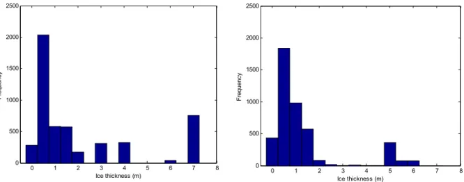
Hourly values for maximum ice thickness for the 1985-86 winter season at Amauligak can be obtained from the CLIP database. The frequency of the thicknesses is shown in Figure 3. Weighted average ice thickness values were also calculated from hourly observations of ice types and concentrations, and are shown below. Relatively stationary 7m thick multiyear floes were present for part of the season, as shown in Figure 3 (graph on left). Other ice types were also present at this time, resulting in lower overall average ice thicknesses (right).

Figure 3 Hourly ice thickness observations: maximum ice thicknesses (left); weighted average ice thicknesses (right)

LOCAL PRESSURES ON MOLIKPAQ

The data from Medof panels can be interpreted as an average pressure on the area of the panel. The Molikpaq data in CLIP have been presented in terms of force per unit width. The forces from two or three vertically adjacent panels can be summed to obtain a line load, i.e. a force per unit width. For each hour, the ice thickness is recorded, and this value can be divided into the line load to yield a local ice pressure. An example of the determination of design area for pressures on one Medof panel group (E2) is shown below in Figure 4. If the maximum line load is on panels 1027 and 1029, the area A1 is used for pressure-area calculations. This area is equal to the

panel width multiplied by the ice thickness. For 2m thick ice, A1 = (1.135m) * (2m) ≈

2.3 m2.

Figure 4 Area determination

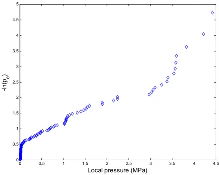
An example of a distribution of peak hourly local pressures on the East face of the Molikpaq is shown in Figure 5. This Weibull plot shows pressures for 1m thick ice (design area of 1.135m2), calculated using the method described above. Note that 46% of the hourly maximum local ice pressures were less than 0.1 MPa.

0 1 2 3 4 5 6 7 8 0 500 1000 1500 2000 2500 Ice thickness (m) F req ue nc y 0 1 2 3 4 5 6 7 8 0 500 1000 1500 2000 2500 Ice thickness (m) F requ enc y

1 0 0.5 1 1.5 2 2.5 3 3.5 4 4.5 0 0.5 1 1.5 2 2.5 3 3.5 4 4.5 5

Local pressure (MPa)

-l

n

(p e

)

Figure 5 Local pressures on the East face of Molikpaq for 1m thick ice Pressures on areas calculated with the method described above are shown in Figure 6 for the East face, and in Figure 7 for the North face. Maximum and average peak hourly pressures were calculated for each value of ice thickness. As shown below, pressures as high as 10 MPa were experienced on areas of approximately 0.45 m2. On areas greater than 3 m2, maximum pressures are about 1 to 2 MPa.

0 1 2 3 4 5 6 7 8 0 2 4 6 8 10 12 Area (m2) P re s s u re (M P a ) Maximum pressure Average pressure

0 1 2 3 4 5 6 7 8 0 1 2 3 4 5 6 7 Area (m2) P re s s u re (M P a ) Maximum pressure Average pressure

Figure 7 Local pressures on North face of Molikpaq

CALCULATING PEAK FACE LOADS ON THE MOLIKPAQ

Experience has shown that immediately adjacent panels tend to have similar time series. Therefore it is reasonable to add the maximum local loads on immediately adjacent panels to get the maximum group load for each 5-minute interval, essentially assuming that the maximum values of loads for immediately adjacent panels are perfectly correlated. Thus for 5 minute intervals on the north face:

(1) N1avg = 1001avg + 1002avg + 1003avg + 1004avg

N2avg = 1006avg + 1007avg + 1008avg + 1009avg

N3avg = 1011avg + 1012avg + 1013avg + 1014avg

(2) N1max = 1001max + 1002max + 1003max + 1004max … and so on.

Here the lower panel (1010) is not taken into account for analysis, since there is only one lower panel for each face of the structure. Next it is assumed that each panel group represents the load on a 20-m length of the face. It is also assumed that the group load histories are statistically similar, while the means and standard deviations can vary from group to group.

The mean load on a face, µ, is the sum of the means of the three groups on a face: (3) µ = Σ µi = N1avg + N2avg + N3avg

Since a value for standard deviation, σ, is not available, it will be assumed that the difference between the group maximum and group average is a measure of the

standard deviation or spread. For panel group 1, the standard deviation is proportional to (N1max – N1avg). In the below equation, n is a constant and is unknown. For three

independent random processes (i = 1, 2, 3), (4) σ = n (Σ σ i 2)1/2

= ((N1max – N1avg)2 + (N2max – N2avg)2 + (N3max – N3avg)2)1/2

One method of estimating the force is allowing it to be equal to the mean plus the standard deviation (D. Matskevitch, personal communication, 1999). Then the peak face load for 5-minute intervals on the 60 m wide North Face is

(5) Fpeak = [N1avg + N2avg + N3avg + ((N1max – N1avg)2 + (N2max – N2avg)2 +

(N3max - N3avg)2)1/2]*20/(2*1.135)

In the above equation, the term (2*1.1.35) accounts for the width of two Medof panels. This gives the peak load on the North Face at each 5-minute interval. Peak loads for the East face were calculated in a similar fashion.

For both the north and east faces, 99 percent of the loads calculated at 5-minute intervals were less than 50 MN. Approximately 95 percent of calculated east face loads were less than 15 MN, and 95 percent of north face loads were less than 25 MN. For both faces, extreme values of ice loads were of the order of 200 MN. This is comparable to previously-calculated estimates of global loads on the Molikpaq at the Amauligak location (Timco and Johnston, 2004).

There is some built-in conservatism in the Fpeak calculations since we assume that

peak loading occurs simultaneously on the panel groups (i.e. N1, N2, N3) during each 5-minute interval. This is not always the case, and typically adds about 10%

conservatism.

As mentioned previously, the Catalogue of Local Ice Pressures contains data on maximum ice thickness and ice drift speed and direction at hourly intervals. To compare the peak face loads to the data available from the CLIP database, hourly values of peak face load were calculated corresponding to the hourly intervals used in CLIP. To do this, the maximum face load was determined for each hour using the peak face loads for 5-minute intervals, as calculated in the previous section. These maximum hourly face loads are used in the analyses in the following sections.

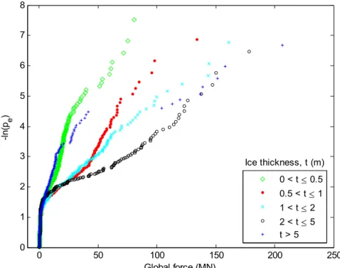
EXCEEDANCE PLOTS FOR ICE THICKNESS AND GLOBAL FACE LOADS For the following analysis, the maximum ice thickness data was used, as it is assumed that thicker ice will generally create greater loads on the structure. Global loads are

sorted by ice thickness and plotted using the Weibull plotting position for the east face (Figure 8) and north face (Figure 9).

0 50 100 150 200 250 0 1 2 3 4 5 6 7 8 Global force (MN) -l n( p e ) Ice thickness, t (m) 0 < t ≤ 0.5 0.5 < t ≤ 1 1 < t ≤ 2 2 < t ≤ 5 t > 5

Figure 8 Probability of exceedance of ice loads on East face of Molikpaq

0 50 100 150 200 250 0 1 2 3 4 5 6 7 8 Global force (MN) -l n(p e ) Ice thickness, t (m) 0 < t ≤ 0.5 0.5 < t ≤ 1 1 < t ≤ 2 2 < t ≤ 5 t > 5

Note that for greater ice thicknesses, the Medof panels may not capture the entire load. The panels are each 2.7m high, so each panel group measures ice loading up to 5.4m vertically. Some of the loading may occur below the panels, which may explain why the distributions in the following figures are not well behaved for ice greater than 5m thick. Some variation can also be expected in the distributions in the following figures since ice information, including thickness, is collected only once per hour (on each whole hour). The face loads take into account pressure data ranging from a half hour before to a half hour after the whole hour. During this period of time, the ice thickness may vary.

PRELIMINARY ESTIMATES OF DESIGN FACE LOAD

Table 1 summarizes the approximate expected values of global load on the 60m wide structure, for each value of ice thickness. Expected face loads are calculated for the appropriate value of probability of exceedance (pe) by fitting a best-fit line to the tail

of each distribution.

As expected, thicker ice generally corresponds to higher ice loads on both the east and north faces. However for the thickest ice (greater than 5 m), this is not the case. As mentioned previously, thick multi-year floes were present for part of the season and had very little movement against the structure. Lower forces than expected may have been exerted on the faces of the structure due to less ice drift for very thick ice. Less ice movement means less exposure to ice, thus a lower probability of high loads on the structure.

Table 1 Estimated global loads on east and north faces of Molikpaq

East face North face

Face load (MN) Face load (MN)

Ice thickness, t (m) Amount of drift (km) pe = 10-2 pe = 10-3 Amount of drift (km) pe = 10-2 pe = 10-3 0 < t ≤ 0.5 850 30 75 133 25 50 0.5 < t ≤ 1 123 60 130 24 70 130 1 < t ≤ 2 174 90 170 80 105 200 2 < t ≤ 5 76 120 190 49 140 190 t > 5 1.6 100 220 0.2 90 190 SUMMARY

Data from the Amauligak I-65 deployment of the Molikpaq for the winter of 1985/86 cover a variety of ice conditions and provide a good basis for establishing exposure criteria. Over the eight and a half month measurement period, more than 60,000 5-minute interval readings of local loads on the Medof panels are available.

For Molikpaq at the Amauligak location, the NRC ‘Catalogue of Local Ice Pressures’ includes hourly observations of ice and meteorological conditions, such as maximum ice thickness and drift speed and direction. One-hour maximum values were obtained

for local ice forces on Medof panels. The Medof panel data in CLIP have been presented in terms of force per unit width. The forces from two or three vertically adjacent panels can be summed to obtain a line load. The ice thickness can be divided into the line load to yield a local ice pressure.

Local pressures up to 10 MPa are calculated for small areas (0.45 m2). On areas greater than 3 m2, pressures are below 2 MPa.

A method is presented for the calculation of peak global loads on the north and east faces. Local ice loads are extracted from the CLIP database and used to obtain estimates of global loads on the north and east faces of Molikpaq. For both the north and east faces, 99 percent of the loads calculated at 5-minute intervals were less than 50 MN. Maximum hourly values of face loads are also calculated, for comparison with the CLIP data on ice thickness.

ACKNOWLEDGEMENTS

The financial support and interest of the CLIP Joint Industry Project participants, (Chevron Canada Resources, ExxonMobil Upstream Research Company, Husky Oil Operations Ltd. and Petro Canada, Transport Canada, the Program of Energy

Research and Development, and the CHC) is greatly appreciated. The support of the participants of the project Ice Data Analysis and Mechanics for Design of Offshore Structures (NSERC, NRC, Petro-Canada, Husky, Chevron, and Memorial University of Newfoundland) is also gratefully acknowledged.

REFERENCES

Frederking, R., and Collins, A., 2005. NRC Catalogue of Local Ice Pressures (CLIP). Canadian Hydraulics Centre Technical Report CHC-CTR-037.

Metge, M., Pilkington, R., Strandberg, A. and Blanchet, D., 1983. A new sensor for measuring ice forces of structures: laboratory tests and field experience. Proceedings 7th International Conference on Port and Ocean Engineering Under Arctic

Conditions, POAC ’73, Helsinki, VTT Symposium 28, Vol. 4, p. 790-801. Timco, G.W. and Johnston, M., 2004. Ice loads on the caisson structures in the Canadian Beaufort Sea, Cold Regions Science and Technology Vol. 38, pp. 185-209.