READ THESE TERMS AND CONDITIONS CAREFULLY BEFORE USING THIS WEBSITE. https://nrc-publications.canada.ca/eng/copyright
Vous avez des questions? Nous pouvons vous aider. Pour communiquer directement avec un auteur, consultez la première page de la revue dans laquelle son article a été publié afin de trouver ses coordonnées. Si vous n’arrivez pas à les repérer, communiquez avec nous à [email protected].
Questions? Contact the NRC Publications Archive team at
[email protected]. If you wish to email the authors directly, please see the first page of the publication for their contact information.
NRC Publications Archive
Archives des publications du CNRC
This publication could be one of several versions: author’s original, accepted manuscript or the publisher’s version. / La version de cette publication peut être l’une des suivantes : la version prépublication de l’auteur, la version acceptée du manuscrit ou la version de l’éditeur.
Access and use of this website and the material on it are subject to the Terms and Conditions set forth at
The Parallel Iterative Closest Point Algorithm
Langis, C.; Greenspan, M.; Godin, Guy
https://publications-cnrc.canada.ca/fra/droits
L’accès à ce site Web et l’utilisation de son contenu sont assujettis aux conditions présentées dans le site
LISEZ CES CONDITIONS ATTENTIVEMENT AVANT D’UTILISER CE SITE WEB.
NRC Publications Record / Notice d'Archives des publications de CNRC:
https://nrc-publications.canada.ca/eng/view/object/?id=69df0800-3552-4491-9fc8-5cceec080cec https://publications-cnrc.canada.ca/fra/voir/objet/?id=69df0800-3552-4491-9fc8-5cceec080cecNational Research Council Canada Institute for Information Technology Conseil national de recherches Canada Institut de technologie de l'information
The Parallel Iterative Closest Point Algorithm *
Langis, C., Greenspan, M., Godin, G.
June 2001
* published in Proceedings of the Third International Conference on 3D Digital Imaging and Modeling (3DIM), Québec City, Québec, Canada. May 28- June 1, 2001. NRC 44184.
Copyright 2001 by
National Research Council of Canada
Permission is granted to quote short excerpts and to reproduce figures and tables from this report, provided that the source of such material is fully acknowledged.
The Parallel Iterative Closest Point Algorithm
Christian Langis
Michael Greenspan
Guy Godin
Visual Information Technology Group
Institute for Information Technology, National Research Council Canada
Bldg. M-50, 1500 Montreal Rd., Ottawa, Ontario, Canada, K1A 0R6
email: firstname.lastname@
nrc.ca
Abstract
This paper describes a parallel implementation developed to improve the time performance of the Iterative Closest Point Algorithm. Within each iteration, the correspon-dence calculations are distributed among the processor re-sources. At the end of each iteration, the results of the cor-respondence determination are communicated back to a central processor and the current transformation is calcu-lated. A number of additional techniques were developed that served to improve upon this basic scheme. Calculat-ing the partial sums within each distributed resource made it unnecessary to transmit the correspondence values back to the central processor, which reduced the communication overhead, and improved time performance. Randomly dis-tributing the points among the processor resources resulted in a better load balancing, which further improved time performance. We also found that thinning the image by randomly removing a certain percentage of the points did not improve the performance, when viewed as the progres-sion of with time. The method was implemented and tested on a 22 node Beowulf class cluster. For a large im-age, linear performance improvements were obtained for up to 16 processors, while they held for up to 8 processors with a smaller image.
1
Introduction
The Iterative Closest Point Algorithm ( ) has be-come established as one the most useful methods of range data processing. Given two sets of partially overlapping range data and an initial estimate of their relative positions, is used to register the data sets by improving the po-sition and orientation estimate. First described by Besl and McKay [1], is an essential step in model building, di-mensional inspection, and numerous applications of range data processing.
At each iteration, correspondences are determined between the two data sets, and a transformation is
com-puted which minimizes the mean square error ( ) of the correspondences. The iterations continue until either the falls below some threshold value, the maximum number of iterations is exceeded, or some other stopping condition is satisfied. Due to its fairly large computational expense, is typically considered to be a batch or, at best, a user-guided online process where the user initiates and assists the process and then allows it to execute unsu-pervised for a number of minutes. An which executes in real-time, or near real-time, would prove advantageous in several situations. One reason is that range data acqui-sition sensors are getting faster. The combination of real-time range data acquisition with a real-real-time forms the basis of a number of new and useful systems, such as geometric tracking and hand-held sensors. Furthermore, there are emerging applications such as environment mod-eling where the volume of data is large, and for which any improvement in the speed of is desirable.
There has been some previous work in developing ef-ficient versions of . Simon et al. [2] implemented efficient correspondence calculations based upon the k-d tree and decoupled acceleration for the rotation and trans-lation components. Jasiobedzki et al. [3] implemented and compared a variety of model representations and cor-respondence methods. Greenspan and Godin [4] proposed a correspondence method which is specifically tailored to efficient .
A generic method for speeding up computations is
par-allelization. There has been a recent resurgence in the pop-ularity of parallel computing, which can be attributed to the improved availability, ease of use, cost effectiveness, and power of PC clusters. Images are an inherently parallel data structure, and image processing methods are likely to benefit directly from the proliferation of parallel comput-ing systems. In this work we describe a parallelized ver-sion of the which we call . The parallelization
scheme proposed here is coarse grain, in that tens of thou-sands of operations or more are executed by each parallel resource between any synchronization or communication. But it is likely that some of the techniques that we present here also apply to the fine grain case.
The objective of parallelization is to approach linear im-provement, i.e. if it takes time to execute using a single processor, we would like it to take only time for processors. While some methods are mired in the sequen-tial framework and seem not to be amenable to paralleliza-tion, others parallelize trivially. If a method is paralleliz-able, then there are two general design principles which must be followed to maximize speedup. The first is to re-duce the ratio of communications to computation. The sec-ond is to balance the computational load equally among the resources.
This paper continues with a description of the basic method in Section 2. In Section 3, a number of techniques are described which aim at improving upon the basic , including parallelized computation of cross-covariances, shuffling, thinning, and acceleration. A set of experiments are reported in Section 4 which characterize the performance of the method. The paper concludes in Section 5 with a summary and a discussion of future re-search.
2
Basic method
The algorithm iteratively registers a floating (i.e.
data) surface towards a reference (i.e. model) surface. In the original description of the method [1], the surfaces can be described by a number of representations, such as point sets, line segments, triangle sets, etc. The only requirement is the existence of a closest point operation which returns, for a given query point, the point on the reference surface that is closest to the query point.
In this work, we consider the case where both surfaces are described as 3D point sets. The decision to restrict ourselves to this geometric representation was motivated by the objective of developing a process which performs registration between range images in real-time as they are acquired. Nevertheless, the parallelization techniques pre-sented here generalize directly to the use of other surface representations, and some other registration methods.
Let the floating and reference images be respectively denoted as and . The basic algorithm is well known [1], but we restate it briefly here for completeness:
1. Establish correspondences: the closest point on the surface of is sought for all points in .
2. Derive transformation: the correspondences are used to compute a transformation matrix which minimizes the mean square error ( ) of the residuals. 3. Transform : the transformation is applied to all
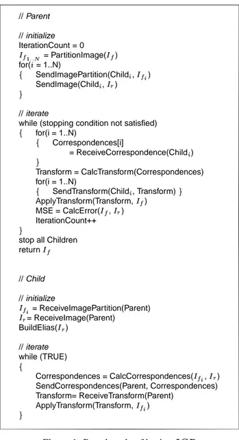
points of . // Parent // initialize IterationCount = 0 = PartitionImage( ) for( = 1..N) SendImagePartition(Child , ) SendImage(Child , ) // iterate
while (stopping condition not satisfied) for(i = 1..N) Correspondences[i] = ReceiveCorrespondence(Child ) Transform = CalcTransform(Correspondences) for(i = 1..N) SendTransform(Child , Transform) ApplyTransform(Transform, ) MSE = CalcError( , ) IterationCount++
stop all Children return // Child // initialize = ReceiveImagePartition(Parent) = ReceiveImage(Parent) BuildElias( ) // iterate while (TRUE) Correspondences = CalcCorrespondences( , ) SendCorrespondences(Parent, Correspondences) Transform= ReceiveTransform(Parent) ApplyTransform(Transform, )
Figure 1: Pseudocode of basic
4. Terminate: if the change in falls below a preset threshold, then terminate. Else, repeat from step 1. The metric which is used to evaluate the good-ness of the registration is the average of the squared dis-tances between corresponding points, i.e. the average of the square of the residuals. It has been shown that if the transformation derived in step 2 minimizes the of the residuals, then the is bound to reduce monoton-ically over the iterations. The iterative structure of the al-gorithm imposes that any parallelization must take place within each iteration.
Within an iteration, establishing the correspondences accounts for the largest portion of the processing expense, and is the most likely candidate for parallelization. Effi-ciently determining the closest point from a set of
possi-bilities is a classical problem of Computational Geometry called the Nearest Neighbor Problem. A variety of practi-cal solution methods exist, such as k-d tree [5] or Elias (or voxel-binning) methods [6], which greatly reduce the cost of establishing correspondences over exhaustive searching. In our tests, we have used a straightforward implementa-tion of the Elias which we found to be very time efficient when compared to the k-d tree method [4]. Regardless of the method used, a nearest neighbor must be found for ev-ery points of the floating image . Hence, the most nat-ural strategy parallelizes the correspondence step by parti-tioning into subsets across the processes.
2.1
Parallelization
A pseudocode representation of the basic parallelized version of the method is depicted in Fig. 1. At initializa-tion, the complete reference image is sent to each of the
childprocesses. The parent process partitions into disjoint subsets , and transmits each subset to a child process. At each iteration, each child process establishes the correspondences between its and , and sends the correspondences back to the parent. The parent then cal-culates the incremental transformation and sends it to the children, which apply it to their in preparation for the next iteration. The basic is composed of the follow-ing operations:
Data partition:The parent process partitions into disjoint subsets. Since the correspondence search time of each subset increases linearly with the number of points in the subset, dividing into subsets of approximately equal cardinality should distribute the workload almost evenly across the child processes.
Initial data transmission: The parent transmits a sub-set to each child process. Each child will work exclu-sively on this subset throughout the registration. Although this initial communication is intensive, it fortunately oc-curs only once every call.
Parallel iterations: Each child concurrently computes the correspondences between points in and the points of . The resulting correspondences are then sent back to the parent process.
Sequential parent computations: Once it receives all correspondences from the child processes, the parent then derives a transformation as in the sequential . At little additional expense, the parent also applies the transforma-tion to its copy of and computes the .
Transformation redistribution: The parent process then transmits the transformation back to the children. The children apply the received transformation to their , thus keeping the distributed copy of consistent with the par-ent’s copy. The parent will stop the iterative process when-ever the requested registration accuracy, or some other con-dition such as a maximum number of iterations, has been
met.
3
Enhancements to the parallel method
At this point, the runtime behaves linearly in terms of (the number of child processes) up to a certain limit of processes, which is characteristic of parallel ap-plications. As increases, the relative cost of communi-cations becomes dominant. Also, the time limiting factor for an iteration is always determined by the slowest pro-cess. Thus the basic can be enhanced by reducing the amount of interprocess communications and by load balancing. A further approach to performance enhance-ments is to reduce the total amount of computations using subsampling of the data and parametric acceleration. The particulars of each of these solutions, along with their rel-ative impact, are presented here.
3.1
Quaternion method
In the simple method outlined in Figure 1, the child processes must transmit at each iteration the list of corre-spondences for their subset to the parent. Derivation of the transformation requires the traversal of the correspon-dence pairs to compute their centroids as well as a matrix from terms of the cross-covariance matrix of the pairings [7].
Explicit transmission of the correspondence informa-tion results in considerable data traffic and introduces a sig-nificant time expense per iteration. Furthermore, sequen-tial addition of the residuals on the parent node does not make use of the available parallel processing power.
A first improvement to the basic parallelization dis-tributes the calculation of the cross-covariance terms across the children. After calculating the local correspon-dences for their subsets of , each child process computes partial sums, which are then sent to the parent and com-bined into the total cross-covariance matrix.
This modification of the method has three positive ef-fects on performance. First, it significantly reduces the amount of data which must be exchanged between the chil-dren and the parent at each iteration: the basic scheme re-quired the transmission of a total of integers (the indices of the corresponding points) at each iteration, whereas the proposed modification requires only values. Sec-ondly, the amount of communication per iteration becomes independent of the size of the images being registered. Thirdly, the degree of parallelism is increased by dividing the burden of the computation of cross-covariance terms among the child processes.
For notation simplicity, the modification to the basic method is described here in general terms for a set of pairings , with points represented as column vec-tors of dimension . With the method, these pairs are those found between and at each iteration.
We are seeking the rigid transformation that minimizes . It is computed using the quaternion-based least squares method [7], which requires computa-tion of the centroids and cross-covariance matrix of the two point sets, from which matrix is computed. The centroids of the paired points are defined as:
(1)
respectively, and the cross-covariance matrix as:
(2)
In the parallelized scheme, the set of pairings is broken into disjoint subsets, each of cardinality , with pair-ings noted as . As well, the centroids for each subset are defined as and . The sum of Eq. 2 can be broken into partial sums ; the computation of can then be rewritten as:
(3)
where the centroids and are computed as:
(4)
Each child reports 16 values to the parent: the second-order elements of , centroid elements, and
, the number of pairs in the subset. In the specific case of the , if all query points in a subset produce a pair-ing, then only 12 values per child need to be transmitted, since remains constant, and the updated centroids of the query points in each subset are readily available to the parent node.
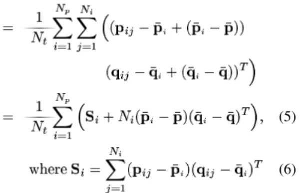
Although the expression in Eq. 2 is algebraically cor-rect, it may be subject to numerical errors for large num-bers of points when the centroid is far from the origin, due to the subtraction of two potentially large terms. The fol-lowing alternative version avoids this potential difficulty at a minimal additional computational cost on the parent pro-cessor:
(5)
(6)
The global centroids are obtained from using Eqs. 4.
In this improved method, almost all computations are parallelized. After finding the pairs, each child com-putes the centroids and . Then, the local cross-covariance matrix (that is, relative to and ) is com-puted (Eq. 6). Each child sends to the parent, which combines them sequentially using Eq. 5. The rigid transformation for all pairs can finally be estimated with the method in [7].
This simple optimization brought a tangible difference in the execution times of our algorithm. Relieved from heavy communications at every iteration, the algorithm shows significant speedup throughout iterations. The dif-ference in time between the parallelized and the sequential computations methods is shown for a typical run in Fig. 2.
0 10 20 30 40 50 60 0 5 10 15 20 25 30 35 40 Time(sec) Iterations Sequential Parallel
Figure 2: Sequential vs. parallel computation of cross-covariances.
3.2
Shuffling
At initialization of the , the floating image is divided into subsets , one for each child process. The subsets are of equal size, in an attempt to balance the work-load evenly across all children. This balancing is crucial to the global performance of the , since one iteration
cannot start before all the children have completed the pre-vious one. Were the correspondence computation a con-stant time operation, then any equal division of the points between processes would indeed achieve the goal. How-ever, this is not the case in general.
The correspondence computation is a Nearest Neighbor problem, which is a classical problem of Computational Geometry for which a variety of solution methods exist, such as k-d tree and Elias methods (e.g. [5, 6]). A com-mon property of most of these methods is that they tend to execute with increasing efficiency as the actual distance to the nearest neighbor decreases. The calculation will there-fore execute more efficiently for regions of for which the residuals to are smaller on average.
The images used here were acquired using a Biris laser range sensor [8] and are ordered as 2D arrays of 3D points, as is typical of imaging range sensors. Thus, points stored contiguously in the image array tend to be located in the same neighborhood of the measured surface.
In our initial implementation, the subsets of were de-rived by simply dividing the image into contiguous blocks. Thus, points would be assigned to child . Under this scheme, some children were as-signed regions of which were either very well or very poorly registered with , leading to an unbalanced work-load. Since the time for an iteration of the is bound by the completion of the slowest of the processes, this issue had to be addressed.
If the points of were uniformly randomly ordered then all subsets of would have approximately the same average residual size for a given iteration, and the cor-respondence computation would bear approximately the same cost across subsets. A simple process known as
shuf-flingwas implemented in an attempt to distribute the work-load more evenly at no additional cost. With shuffling, child is assigned points . Each subset is therefore composed of a set of points uni-formly dispersed across .
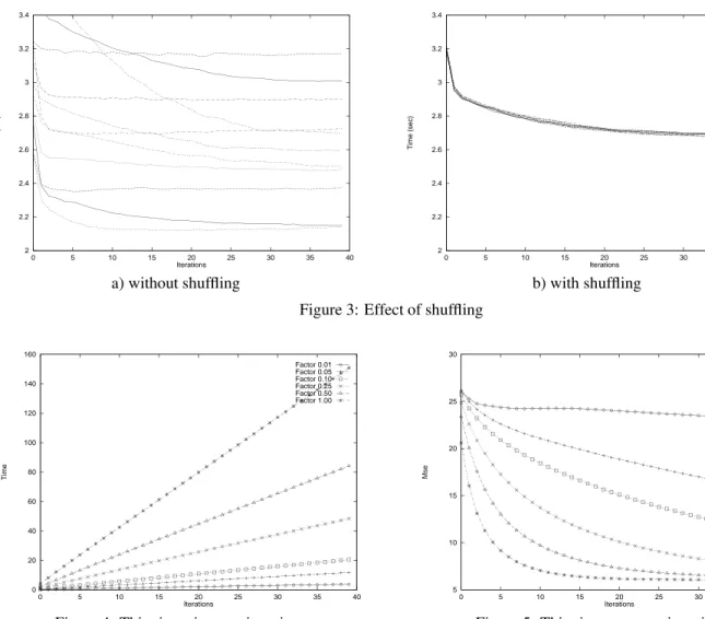
The improvement in the distribution of the workload us-ing shufflus-ing is illustrated in Fig. 3. The was run on the same data set for the same starting conditions with and without shuffling. The graphs show the execution time per iteration for 11 child processes. Clearly in Fig. 3 b) shuf-fling reduces the variation in execution time between pro-cesses, and the curves are tightly grouped together. Signif-icantly, after a few iterations, the total time was reduced by , from 3.2 to 2.7 seconds, when shuffling was ap-plied. The gain is even larger during the first few iterations where the curves exhibit more variability. Shuffling also tends to yield similar centroids of pairings for each child process, which makes Eq. 5 even more numerically stable. However, the experimentations with shuffling did not
always yield positive results. One of the undeniable ben-efits of shuffling is to group together the individual child timings rather than leaving the original point ordering of determining the variance of workload on the children. However, sometimes, there was still no speedup; the slow-est child with shuffling was not any faster than without shuffling.
An interesting behavior was observed when evaluating the aggregate time (sum of all of the 11 individual child times) for each iteration. The aggregate times of the runs with shuffling exceeded those without shuffling by 20%. Our analysis attributed this unexpected performance to a poorer data cache usage. It should be remembered that the aggregate time is not in itself the measure of perfor-mance for a parallel algorithm. It does, however, provide the means for a comparison of the overhead of parallelism between different trials.
Without shuffling, the correspondences for each subset of are rather well localized on a specific region of . However, when the subsets are uniform samples of , their individual correspondences span completely. Hence, the consequence of uniformly distributed subsets is that each child must probe completely, as opposed to a specific region of in the non-shuffled case. And since the Elias data structure for typical images rarely fits completely into the available cache memory, shuffling often causes much lower cache hit rates than the non-shuffled case. For this reason, shuffling must be used with caution, adjusted to the amount of cache available to each child CPU. Mod-ifications of some key data structures used in the Nearest Neighbor computation are under way to alleviate this ef-fect.
3.3
Thinning
Using either the sequential or parallel method, the time to establish correspondences increases linearly with the size of . One is therefore tempted to speed up (and ) by using only a smaller portion of the points in . Masuda and Yokoya [9] used random sampling to remove outliers, and the technique of subsampling has become a common practice to improve computational efficiency.
We evaluated the effect of reducing the size of with a technique called thinning. At the beginning of each iter-ation, the processes randomly subsample their subsets, at a factor . Following the subsampling, only the points selected by the subsampling filter are consid-ered further in the correspondence computations.
To study the effect of thinning, experiments were per-formed using the sequential (i.e. only one child pro-cess) for six values of . Figure 4 plots the cumulative time per run as a function of iterations. As expected, the time per iteration decreases linearly with the value of . In Fig. 5, the is plotted as a function of iterations.
2 2.2 2.4 2.6 2.8 3 3.2 3.4 0 5 10 15 20 25 30 35 40 Time (sec) Iterations 2 2.2 2.4 2.6 2.8 3 3.2 3.4 0 5 10 15 20 25 30 35 40 Time (sec) Iterations
a) without shuffling b) with shuffling Figure 3: Effect of shuffling
0 20 40 60 80 100 120 140 160 0 5 10 15 20 25 30 35 40 Time Iterations Factor 0.01 Factor 0.05 Factor 0.10 Factor 0.25 Factor 0.50 Factor 1.00
Figure 4: Thinning: time vs. iterations
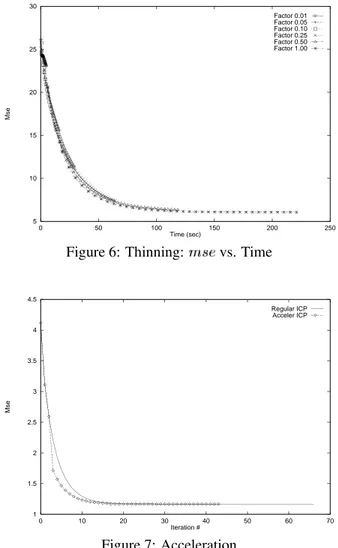
Despite the random subsampling of at the beginning of each iteration, it can be seen that for a given iteration the value is smaller for the more densely sampled subsets. An interesting conclusion can be drawn from Fig. 6, where the evolution of the with time is seen to be nearly identical for all values of . By decreasing the value of , the slower convergence of the almost exactly cancels out the faster iterations. From this graph, it ap-pears that there is no efficiency improvement to be gained by thinning the image.
3.4
Acceleration
Another enhancement which is not specific to the par-allel implementation is parametric acceleration [1]. It is a technique that can be applied on top of to quicken the convergence: it does not speedup the execution time of the iterations, but instead skips some of them by applying an extrapolation factor based on the 6D trajectory of the transformation.
Estimation of the acceleration factor does not require
5 10 15 20 25 30 0 5 10 15 20 25 30 35 40 Mse Iterations Factor 0.01 Factor 0.05 Factor 0.10 Factor 0.25 Factor 0.50 Factor 1.00
Figure 5: Thinning: vs. iterations
correspondence computations; its execution time is in-significant compared to that of a single iteration. There-fore, it seems appropriate to take advantage of this tech-nique as much as possible. However, the transforms it de-rives do not follow the monotonic convergence prop-erty. In fact, our particular implementation of accelera-tion showed that very few accelerated transforms yielded smaller . Nevertheless, this does not prevent its use since a disadvantageous acceleration step can simply be discarded.
The best result is shown in Fig. 7. The acceleration pa-rameters were especially tuned for this data set (for max-imum acceleration). The two curves show the con-vergence for accelerated and non-accelerated runs. Both curves appear superposed until iteration 4, where the acceleration kicks in and drives the lower on the ac-celerated curve. This was the only beneficial acceleration for this registration run. Furthermore the non-accelerated curve catches up quickly with the accelerated one in the
5 10 15 20 25 30 0 50 100 150 200 250 Mse Time (sec) Factor 0.01 Factor 0.05 Factor 0.10 Factor 0.25 Factor 0.50 Factor 1.00
Figure 6: Thinning: vs. Time
1 1.5 2 2.5 3 3.5 4 4.5 0 10 20 30 40 50 60 70 Mse Iteration # Regular ICP Acceler ICP Figure 7: Acceleration
region of the figure where convergence slows down heavily. In this figure, acceleration eliminated about 20 it-erations out of over 60. However, on average with different data sets less than 10% of iterations are spared which is far less performance than what we expected out of the tech-nique.
Further experimentations were also conducted with an-other acceleration method [2]. This method, based on the previous one, breaks up the transformation into rotation and translation, each with a different extrapolation factor. Again, we observed no tangible improvements.
Although acceleration makes sense in theory, experi-mentations showed that a transform slightly off the trans-form trajectory generated with regular iterations causes ev-ident regressions in terms of . Hence such a transform close to the transformation path, might possibly generate a much higher than the first transform in the sequence. Again, our battery of tests was restricted on points clouds data sets. Hence, the results showed in this paper may not be comparable with those of other papers. Baring that,
those results may also be the consequence of an implemen-tation error.
4
Experimentation
All experimentations were performed on a Beowulf class cluster of PCs comprising 24 Pentium II processors connected over a 100Mbps Ethernet switch. The nodes were configured as dual processors so that all CPUs fit within 12 boxes. The system was not completely sym-metric: 9 of the PCs were dual Pentium II 350Mhz with 500MB of RAM, while the remaining 3 were dual Pentium II 450Mhz with 1GB of RAM. All processors were running the RedHat LINUX 5.2 operating system. We were ini-tially inclined to use MPI as the message passing layer, but in preliminary tests, it was found that MPI did not support a true multicasting function. As multicasting was deemed to be important to our application, we decided to use PVM (version 3.3.11) which had an efficient implementation of multicasting and multityped messages.
Tests were run on eight image pairs acquired with a
Birisrange sensor [8]. For the sake of brevity, the results of only two of these test sets are reported here: a large pair ( , ), and a small pair ( , ). The results of the other image tests followed a pattern similar as those presented here, and led to the same conclusions. These images contained sufficient variation in shape so that they did not register trivially, and were considered to represent typical test cases.
Eighty iterations of the were executed for each image pair for a varying number of child processes,
. Note that the total number of processors available in the system was 24, one of which was required for the parent process. The additional CPU which shared the same motherboard as the parent process CPU was not used, so that symmetry of the child processes was maintained.
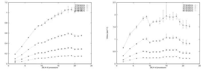
A graph of the large and small image pair tests are re-spectively illustrated in Figures 8a) and b). The graphs show the system speed, defined as the inverse of the execu-tion time as a funcexecu-tion of . The curves are the average of five different test runs with error bars indicating the mini-mum and maximini-mum values between runs.
The large data plot (Fig. 8a)) shows that up to
the speed improvement is nearly linear in the number of child processes. For , the performance begins to degrade. The same effect is observed in the small data plot, but commencing at . In both cases, this degradation was believed to be caused by the increase in the commu-nication overhead as increased. The values of
and therefore represent the limitations of the granularity of this implementation of the parallel method on this system architecture for the respective data sets. It is be-lieved that the observed limitations on the granularity will be similar for data sets of similar size, and this behavior
0 0.2 0.4 0.6 0.8 1 1.2 0 5 10 15 20 25 1/time (sec^-1) (N) # of processors 10 iterations 20 iterations 40 iterations 80 iterations 0 0.5 1 1.5 2 2.5 0 5 10 15 20 25 1/time (sec^-1) (N) # of processors 10 iterations 20 iterations 40 iterations 80 iterations
a) Large Image ( ) b) Small Image ( ) Figure 8: vs. speed (inverse of time)
was indeed observed on the other data sets that were tested.
5
Conclusions
We have presented , a parallel implementation of which has achieved a linear speedup for up to 18 pro-cessors for an image of size points. For a smaller image of size points, the speedup was linear for up to 8 processors.
A number of enhancements were developed to im-prove the performance over that of the basic parallelization scheme. By distributing the cross-covariance calculation, it was possible to considerably reduce the communication overhead, which realized a speedup of in some runs. Shuffling the image served to better balance the load among the processes, which improved performance by an-other . It was also found that a straightforward ap-plication of image thinning did not have any beneficial ef-fects. While the iterations were certainly faster, the rate of reduction of the registration error did not improve. This result was deemed to be significant, as it was both counter-intuitive, and contrary to popular belief.
The amount of communication per process was quite small, and so the ultimate breakdown in linearity was at-tributed to specifics of the current networking system. It is believed that faster switches (which are currently available) or a different machine architecture (such as a shared mem-ory machine) would reduce this effect so that the region of linearity could be extended over a much larger number of processes. Experiments on fine grain parallel systems are planned to assess the efficiency of the on such architectures.
References
[1] Paul J. Besl and Neil D. McKay. A method for registration of 3d shapes. IEEE Trans. PAMI, 14(2):239–256, February 1992.
[2] David A. Simon, Martial Hebert, and Takeo Kanade. Real-time 3-d pose estimation using a high-speed range sensor. In IEEE Intl. Conf. Robotics and Automation, pages 2235– 2241, San Diego, California, May 8-13 1994.
[3] Piotr Jasiobedzki, Jimmy Talbot, and Mark Abraham. Fast 3d pose estimation for on-orbit robotics. In ISR 2000: 31st Intl. Symposium on Robotics, pages 434–440, Montr´eal, Canada, May 14-17 2000.
[4] Michael Greenspan and Guy Godin. A nearest neighbor method for efficient icp. Submitted to the 3rd Int. Conf. on Three-Dimensional Imaging and Modeling, 2001.
[5] Jon Louis Bentley. Multidimensional binary search trees used for associative searching. Communications of the ACM, 18(9):509–517, September 1975.
[6] Ronald L. Rivest. On the optimality of elias’s algorithm for performing best-match searches. In Information Processing 74, pages 678–681, 1974.
[7] B.K.P. Horn. Closed-form solution of absolute orientation using unit quaternions. Journal Optical Society of America A, 4(4):629–642, April 1987.
[8] Franc¸ois Blais and Mario Lecavalier. Application of the Biris range sensor for volume evaluation. In Optical 3-D Measure-ment Techniques III, pages 404–413, Vienna, Austria, Octo-ber 2-4 1995.
[9] T Masuda and N. Yokoya. A robust method for registration and segmentation of multiple range images. Computer Vision and Image Understanding, 61(3):293–307, 1995.