Case study of a 39-story building : model verification and performance comparison with a semi-active device

(1)

Case Study of a 39-Story Building: Model Verification and

Performance Comparison with a Semi-active Device

by

Fernando Pereira-Mosqueira Ingeniero de Caminos, Canales y Puertos

Universidade da Corufia, 2008 ACNES

SUBMITTED TO THE DEPARTMENT OF CIVIL AND ENVIRONMENTAL ENGINEERING IN PARTIAL FULFILLMENT OF THE REQUIREMENTS FOR THE

DEGREE OF MASTER OF ENGINEERING IN CIVIL AND ENVIRONMENTAL ENGINEERING AT THE MASSACHUSETTS INSTITUTE OF TECHNOLOGY

JUNE 2010

MASSACHUSETS INSnitijT OF TECHNOLOGY

JUL 15 2010

LIBRARIES

The author hereby grants to MIT permission to reproduce and to distribute publicly paper and electronic copies of this thesis document in whole or in part in any medium now

known or hereafter created.

Signature of Author:

DepartmentoiC il and Environmental Engineering May 14, 2010 Certified by:

Jerome J. Connor Professor of Civil and Environmental Engineering Thesis Supivisor

Accepted by: _.0e

C n ane Stdezino

(2)

Case Study of a 39-Story Building: Model Verification and Performance Comparison with a Semi-active Device

By

Fernando Pereira-Mosqueira

Submitted to the Department of Civil and Environmental Engineering on May 14, 2010 in Partial Fulfillment of the Requirements for the Degree of Master of Engineering in Civil

and Environmental Engineering at the Massachusetts Institute of Technology.

ABSTRACT

Implementing viscous dampers in high-rise buildings has proven to be an efficient structural way to control interstory drift and accelerations in buildings undergoing wind and earthquake excitations. However, the cost of this implementation sometimes turns to be prohibitive or too high. As a possible more economic solution, this paper introduces the use of a semi-active device to approach this kind of problems. A 39 story building computer model is fully developed. Static and dynamic characteristics of the model obtained are compared with the data obtained from the original design and the wind tunnel results in order to show the accuracy of the computer model. Finally, a comparative study of the efficiency of Modified Friction device and passive dampers under wind excitation is carried out.

Thesis supervisor: Jerome J. Connor

(3)

ACKNOWLEDGMENTS

The author would like to acknowledge Dr. Robert McNamara and McNamara/Salvia Inc. for their help with providing data for the simulated structure. The author would also like to thank Simon Laflamme for his help and advice throughout the whole duration of the study. Finally, the author would like to express his gratitude to Professor Jerome J. Connor, Mohamed Abdellaoui Maane, Geoffroy Larrecq, Alexander Graybeal, my parents and Lucia for their help and support at different stages of this thesis.

(4)

LIST OF FIGURES

Fig. 1 General viscous damper scheme (R. a. McNamara 2003) ... 9

Fig.2 Detailed viscous damper scheme (R. a. McNamara 2003) ... 10

Fig. 3 Viscous damper and diagonal framing conceptualization... 11

Fig. 4 Detailed viscous damper scheme (content.answers.com s.f) ... 11

Fig. 5 Dashpot response under periodic excitation Fig. 6 Coulomb device under periodic excitation... 12

Fig. 7 Coulomb and dashpot system under periodic excitation... 12

Fig. 8. VOD conceptual model extracted from (Connor 2002)... 14

Fig. 9 Scheme for a M R damper (Choi 2001)... 15

Fig. 10 MR damper and diagonal framing conceptualization ... 15

Fig. 11 MR Damper response under sinusoidal loading (Larrecq 2010)... 16

Fig. 12 MFD Duo-Servo drum brake scheme (Laflamme 20 10) ... 17

Fig. 13 MFD conceptualization (Laflamme 2010)... 17

Fig. 14 MFD damper response under sinusoidal loading (Abdellaoui 2010) ... 18

Fig. 15. Flowchart for a controlled system ... 19

Fig. 16 Clipped rule decision schem e ... 21

Fig. 17. SAP2000 structural model for the X and Y directions ... 23

Fig. 18. Stiffness extraction from a 3D frame model for the X direction ... 24

Fig. 19. Periods of vibration for the lumped model... 25

Fig. 20 W ind load tim e history ... 26

Fig. 21 Maximum acceleration profile for X direction ... 30

Fig. 22 Maximum acceleration profile for Y direction ... 31

Fig. 23 Viscous damper behavior between 17th and ₁₈th floor for X Direction ... 31

Fig. 24 MFD behavior between 17th and ₁₈th floor X Direction ... 32

Fig. 25 Maximum acceleration profile for X direction... 33

Fig. 26 Maximum acceleration profile for Y direction... 34

Fig. 27 MFD behavior between 17th and ₁₈th floor X Direction ... 34

Fig. 28 Maximum acceleration profile for X direction... 35

Fig. 29 Data Maximum acceleration profile for Y direction... 36 6

(7)

Fig. 30 MFD behavior between 1 7 th and 18th floor X Direction ... 36

Fig. 31. Maximum acceleration profile for X direction... 37

Fig. 32. Data Maximum acceleration profile for Y direction... 38

Fig. 33. MFD behavior between 1 7 th and 1 8 th floor X Direction ... 38

Fig. 34. Maximum acceleration profile for X direction ... 40

Fig. 37. Data Maximum acceleration profile for X direction... 43

Fig. 42. MFD behavior between 17 th and 1 8th floor X Direction ... 46

Fig. 45. MFD behavior between 19th and 2 0th floor X Direction ... 49

Fig. 48. MFD behavior between 19th and 2 0th floor X Direction ... 51

(8)

LIST OF TABLES

Table 1. Damping distribution in the current design ... 10

Table 2. Data extracted from (R. a. McNamara 2003) ... 24

Table 3. Data obtained from the lumped model ... 25

Table 4. Data extracted from (R. a. McNamara 2003) and data obtained from the lumped m o d el... 2 6 Table 5. Data obtained from the lumped model ... 29

Table 6. Work done by the MFD's ... 29

Table 7. Work done by viscous damper scheme ... 30

Table 8.Data obtained from the lumped model... 33

Table 21. Economic evaluation chart for heuristic method ... 52

(9)

1. INTRODUCTION

1.1. BUILDING STRUCTURAL SYSTEM

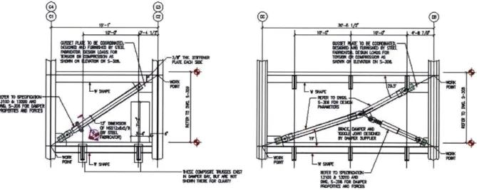
As McNamara described in his paper (R. a. McNamara 2003), the 39-story building can be considered as a moment-frame-tube structural system. In addition to that, diagonal dampers have been placed on every other floor between the 5th and the 3 4th floor in the X direction

(E-W). Regarding the Y direction (N-S), toggle braced damper (TBD) was chosen as the appropriate scheme. The main reason to use TBD was the amplification of the damper stroke achieved and the magnification of the damper maximum capacity.

DAMPER LOCATIONS

FROM EL 81'-6" & ABOVE

Fig. 1 General viscous damper scheme (R. a. McNamara 2003)

9 rd" PW rav raw raq aw RWM. raw raw MW 16 FM raw PAR FW rip fjml , ZZ71 7-7 -7-7-AiMMUMNLOL z

(10)

1.2. DAMPER CHARACTERISTICS

In the next figure from (R. a. McNamara 2003), it is showed the detailed damping implementation for both directions. Both drawings show the connection between damper and the rest of the structure. The design of those connections is fundamental because they need to transfer the loads to the rest of the structure.

+ ~~~7 1ff74~ L

iss p re sened

FMMM Mo FUS

InM next30 the tabl issowtsm a of the toaisoscefiin C (N~m per loo and iretion Fo futherdesripion n trmsof mximm srokeperflor an brcin

angles goE toApni .I h olwigcatr2 h eiiio o icu ofiin

is presented

Floors Cx total Cy total

(kN/m*s) (kN/m*s)

5th to 24th 73904 50165

25th to 34th 49270 25082

Table 1. Damping distribution in the current design

Next chapter describes in depth the nature of viscous dampers (Fig.4) previously described. Furthermore, a conceptual model is developed (Fig.3) and the behavior of this device is described in Fig.5 to Fig.7.

(11)

2. VISCOUS

DAMPERS (PASSIVE CONTROL SYSTEMS)

2.1.

INTRODUCTION

Passive control systems, such as viscous dampers, alleviate energy dissipation demand on the primary structure by reflecting or absorbing part of the input energy, thereby reducing possible structural damage (Housner 1997). Specifically, viscous fluid dampers dissipate

our _{energy by turning kinetic energy (due to velocity) into}

heat. As it can be observed in Fig.3, fluid viscous dampers consist of a piston that moves within a cylinder filled with a viscous fluid that dampen and control motion. A conceptualization of the real model is showed

L

in Fig. 4.

Fig. 3 Viscous damper and diagonal framing conceptualization Fig. 4 Detailed viscous damper scheme (content.answers.com s.f.)

In regards to the conceptual model, one dashpot is the part causing reduction in the kinetic energy while Coulomb/friction stabilizes the behavior of the damper when velocities are close to zero. This friction damper has capacity one or two orders of magnitude smaller than the viscous damper and it can be neglected most of the times.

Fvis =Co * va + F0 * sign(v) (2.1.)

Using this conceptual model, plots of force versus displacement were generated (Fig.5 to Fig.7).

(12)

Several graphs are showed to illustrate the viscous damper behavior under periodic excitation and the effect of the friction damper on the general behavior of the system.

Z 100 . 0 E $A -SW -0.8 -0.6 -04 -0.2 0 0.2 0.4 Displacement (m) 0.6 0.8 1

Fig. 5 Dashpot response under periodic excitation 2000 Z 1500 4)10D 0 U OW ~-1W0 ~-100 -All 15m -Soo 0--15M 1 -08 -0,6 -04 -02 0 0.2 0.4 0.6 0.8 Displacement (m)

Fig. 6 Coulomb device under periodic excitation

- 08 -0.8 -04 -02 0 0.2 0.4 0.6 0.8

Displacement (m)

Fig. 7 Coulomb and dashpot system under periodic excitation

Fig. 7 shows the behavior of the model including a dashpot and a friction device. It is important to point out that the friction device adds certain force to the system when displacement is maximum (dashpot is not able to generate any force in this situation of maximum displacements, Fig. 5). The quantity of force generated by the friction model is, as previously mentioned, one or two orders of magnitude smaller than the dashpot maximum capacity. Hence, the transition of the system through velocities equal to zero is still smooth without the discontinuity that a big friction would generate Fig.7.

(13)

Viscous dampers are classified as passive devices as previously mentioned. Hence, it is interesting to study some kind of devices able to either exert a force into the structure (active devices) or change their characteristics (semi-active devices) depending on the state of the structure. The latter kind of devices is discussed in the following chapter.

(14)

3. SEMI-ACTIVE CONTROL DEVICES

3.1.

INTRODUCTION

Active control devices have showed to be a more efficient way to dampen structural response under extreme events (high wind and earthquake excitations). However, the large energy consumption required during those extreme events has result in development of semi-active control systems. This type of device cannot exert a force into the structure, but their properties can be adapted practically in real time with only a small delay. Instead of using large amounts of energy, these devices can work with only a battery. This is an important issue because dampers must work under extreme conditions when power outages may occur. Among the multiple existing semi-active devices, this thesis covers three of them: Variable-Orifice Dampers, Magnetorheological dampers and modified friction devices.

3.2. VARIABLE-ORIFICE DAMPER (VOD)

This technology is one of the simplest used for semi-active control. It consists in a conventional viscous damper that has installed an additional valve (mechanically controlled) that can vary the resistance to flow for the fluid within the viscous damper (B.F. Spencer 1999). As a result viscous damping coefficient can range from a lower value (valve 100% opened) to a higher value (valve completely closed) depending on the force required to mitigate vibrations. Fig. 8 shows the conceptualization of the device.

(15)

3.3. MAGNETORHEOLOGICAL DAMPERS (MR DAMPERS)

Among this kind of systems, MR Dampers (controllable fluid dampers) are described in this thesis. MR fluids have the special characteristic that under certain magnetic field, they

are able to change from free-flowing, linear viscous fluids to semi-solids with controllable yield strength.

F v Regarding conceptual model, MR is made of a

Magneic I1combination of springs, dashpots and a hysteretic

""" \device _{system Fig. 10.}

x

Ampcro

Fig. 9 Scheme for a MR damper (Choi 2001)

Fig. 10 MR damper and diagonal framing conceptualization

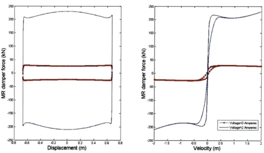
In order to show the change in behavior depending on the voltage applied. A sinusoidal load has been applied on the MR model developed in the thesis (Larrecq 2010). Results are presented in Fig. 11.

(16)

150

100 a50

-. 1-s -004 -0.2 0 0,2 0,4 06 0.

DispIcement (M) -2 -1.5 -1 -0.5 velocity (M)0 05 1 1.5

Fig. 11 MR Damper response under sinusoidal loading (Larrecq 2010)

2M0 150 150 50 0 1w -150 -2W 2hu -

(17)

-o"-3.4. MODIFIED FRICTION DEVICE (MFD)

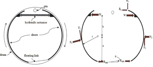
Another type of device, MFD (controllable friction brake), is presented in this thesis. MFD consists of one drum. Inside this drum, a hydraulic actuator exerts a force on two shoes designed for this purpose. This results in friction when rotation happens. The capability of changing the normal force exerted on the drum involves changes in the friction characteristics as desired. This makes MFD a really interesting device to consider.

hydraui actuator

4 =

)

oe

r

N2

drum floating link 1

1

Fig. 12 MFD Duo-Servo drum brake scheme (Laflamme 2010)

The scope of the thesis is to get an economical evaluation of the cost of implementing MFD technology in a 39-story building to compare against the estimated cost of the classical

dashpot element

stiffness

element

variable friction element

, v saJU3 arIIFp,]A 11peL U11.n.llukal

Regarding conceptual model, MFD is made of a combination of springs, dashpots and a friction + F device system (Fig. 13).

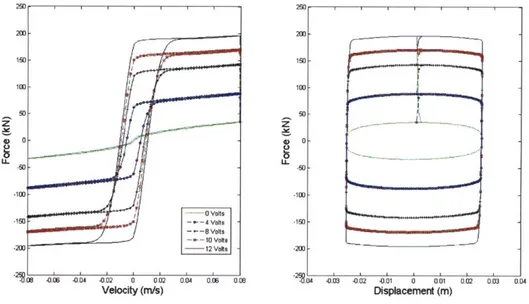
In order to show the change in behavior depending on the voltage applied (0-12 volts). A sinusoidal load has been applied on the MFD model developed for this purpose (Abdellaoui 2010). Results are presented in Fig. 14.

-+x

Fig. 13 MFD conceptualization (Laflamme 2010)

.. .. .. .. .. .. ..

(18)

The total force exerted by the MFD is a combination of friction, spring and dashpot forces. Expression for this total force is presented in the next formula (3.1.):

F = Ffriction + kmfd * X + Cmfd * X (3.1.)

It is really important to consider for this device the temperature increase due to heat generated by friction between surfaces. In order to solve this problem, the device proposed in (Laflamme 2010) mixes steel fiber lining with 15% weight ceramic fibers.

Velocity (m/s)

-:.04 -0.03 -002 -001 0 0.01 002 Displacement (m)

Fig. 14 MFD damper response under sinusoidal loading (Abdellaoui 2010)

Previously, the study has covered the change in behavior of semi-active devices depending on the variable valve opening or variable voltage. However, how these conditions are varied has a big effect on the device's general behavior. Controllers are in charge of deciding the required action based on observations of the structure. The following chapter discusses the most common controllers.

(19)

4. CONTROL RULES FOR SEMI-ACTIVE DEVICES

4.1.

INTRODUCTION

Control rules are very important when dealing with active and semi-active devices. These rules are always based on the observations of the system state. Once the observations are measured, the controller decides the action to take and it sends this information to the actuator that acts in consequence to this.

Fig. 15. Flowchart for a controlled system

Regarding structures, based on the observations of the system, the actuator to reduce state in step i+ is obtained.

optimum force required by

Among the multiple optimum force methods, most widely used are: LQR (Linear Quadratic Regulator), H-infinity, and LQG (Linear Quadratic Gaussian). LQR will be discussed in this thesis.

When dealing with active controllers, force required can be directly exerted in the structure (action). However, semi-active devices change properties based on changes in the dynamics of the device (electric field, electromagnetic field or valve orifice) but they cannot exert a force into the structure (they generate a reacting force based on the state of the structure but the can actively change their own dynamics). Hence, the action involves a voltage or valve opening selection. The clipped optimal rule and sliding mode controllers are two controllers discussed in this thesis.

(20)

4.2. LINEAR QUADRATIC REGULATOR

(LQR)

Linear Quadratic Regulator (LQR) optimization is chosen to calculate the force required by the damper. The final aim is to obtain a scalar performance index called J. As a result of minimizing J, gain matrix (Kf) is obtained. This matrix multiplied by the state vector Xi (containing displacements and velocities for every degree of freedom for step i provides the force required by the actuators to minimize the damped response state for step i+1.

1=

XT*Q*X+uT*fN*u (4.1.)

Q

and R are the weight matrices on the state vector (X) and the damper forces (u), respectively. There is no method to obtain optimal values for both control matrices. Following heuristic methods, different weight matrices have to be tested until get the desired performance in the system.

4.2.1. CLIPPED OPTIMAL RULE

Voltage change leads into an important variation in the general damper efficiency. Hence, the control rule, that is going to be implemented in the system, will play a crucial role in the behavior of the damper. Clipped control rule is implemented at the beginning of the research. Its simplicity and high efficiency make this control rule perfect for these first stages.

Involving this clipped rule, optimum force required by the device is used to decide the voltage to apply to the semi-active system.

Once the force required is known, it is compared to the force exerted by the damper at step i. If the force generated by the damper for step i is bigger than the required force, voltage is turned off (0 volts). However, if the force generated by the damper is smaller than the required and the sign of the force is the same than the sign for the velocity of the system, the order is turn on the voltage (12 volts).

(21)

Fig. 16 shows the decision scheme for the clipped rule control used in the first stage of the research. The black area corresponds to maximum voltage while the white corresponds to 0 volts.

required i+1

V=12 Volts

LMFD

V=12 Volts

(22)

4.3.

SLIDING MODE CONTROLLER (LYAPUNOV)

This controller tries to increase the frequency of voltage change in the system in order to increase the efficiency of the device under any circumstance (Laflamme 2010).

This controller is used to control the MFD out of the hysteresis area (velocity close to zero). The final aim is to generate the force required by the LQR. Error is defined as e=Fact-Freq.

Ideally, this error would tend to zero. However, the device does not have enough capacity to generate the Freq for every state. Hence, voltage is selected in order to minimize this error

as much as possible.

Using the squared standard deviation and deriving it, it is obtained the minimum for this function.

V - 2 (4.2.)

2

V =e - (4.3.)

V = e [Fact - Freq] (4.4.)

In (Laflamme 2010) it is said that to ensure the negative definiteness of the Lyapunov function (4.2.), the control voltage can be chosen such that:

vreq=vact + 0 -Ee) sign(x) (4.5.)

Tr Fc,0

where X, X and X represent the state of the system. , represents the system uncertainty and 11 represents the delay of the voltage. The other factors in the equation are intrinsic to the MFD nature. To get the complete mathematical basis for this control method, consult (Laflamme 2010).

(23)

5. MODEL VERIFICATION

5.1.

MASS AND STIFFNESS MATRIX EXTRACTION METHODOLOGY

The SAP2000 structural model is used as a base for the structure stiffness and mass extraction. First, ultra-stiff elements are added to the model to lump the behavior of every floor in a single 3 degree of freedom (DOF) element which is going to contain the stiffness in the X and Y direction plus rotation in Z axis (torsion). Furthermore, the mass of the whole story is lumped at those points. Known that the ultra-stiff additional elements are going to introduce unrealistic stiffness in the model, the final stiffness matrix (K) obtained is proportionally scaled to obtain the dynamic and static behavior of the initial model (deflection subjected to static loading, periods of vibration and mass participation factors).

Fig. 17. SAP2000 structural model for the X and Y directions

The methodology used to extract the stiffness matrix consisted in restraining interstory movements and rotations. Afterwards, unitary displacement at the top of each floor, for every desired direction (X, Y and Z rotation), is applied. As a result, the reactions obtained in the floor are equal to the stiffness of this floor in the direction were the displacement is applied (Fig. 18).

(24)

x=1

F

Fig. 18. Stiffness extraction from a 3D frame model for the X direction

In the paper developed by (R. a. McNamara 2003), 1% proportional damping was chosen for the building undergoing seismic excitation. In this thesis, 5.26 and 5 seconds have been chosen calculate the Rayleigh proportional damping (matching the first two periods of vibration for the structure). This results in coupled (complex) eigenvalues for the structure.

5.2.

MODAL ANALYSIS COMPARISON

As described in the previous chapter, K matrix was scaled in such a way that the static deflection was similar to the one obtained for the initial structural model. After this step, first 6 periods of vibration and mass participation factor were extracted, yielding the following results. Final stiffness, mass and damping matrix are presented in Appendix B (building structural properties).

Table 2. Data extracted from (R. a. McNamara 2003)

Mode Shape 1 2 3 4 5 6

Period (sec) 5.26 5.00 3.65 1.92 1.82 1.71

Effective Mass(%) 66.1 62.6 81.2 15.3 12.8 8.5

(25)

Mode Shape 1 2 3 4 5 6

Period (sec) 5.27 4.97 3.63 2.15 2.05 1.73

Effective Mass (%) 65.62 63.69 66.04 15.15 14.77 25.85

Direction X (E-W) Y (N-S) Rotation X (E-W) Y (N-S) Rotation

Table 3. Data obtained from the lumped model

4

03

(-Natural periods of vibration

b 5.28 05,00 @364 @216 _@ 2 07 _1,82 1 2 3 4 5 Mode of vibration 6 7

Fig. 19. Periods of vibration for the lumped model

5.3. LOAD CASES

5.3.1. WIND LOAD

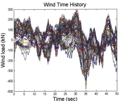
Regarding wind loads, just time history acceleration at the roof is available in the literature. Because of this, loading cannot be extrapolated to generate the same simulation. Data available from another similar structure (Fig. 20) has been used. The peak wind load is scaled in such a way that the same peak acceleration will be generated on the 37th floor, as the one provided in the literature (R. a. McNamara 2003).

(26)

Wind Time History

, , , IA I 300 , 200 1W -100 C-200--300 M 2 X

Time (sec)

Fig. 20 Wind load time history

5.4. RESULTS

Wind tunnel Lumped Lumped

results model model

E-W (X) Dir. E-W (X) Dir. N-S (Y) Dir. N-S (Y) Dir

Response without dampers Response with dampers accel. at 37th Flr. (M/S2) displ. at 3 7th Flr.(m/s) Base Shear (kN) accel. at 37th Flr.(m/s 2 ) displ. at 3 7h Flr.(m/s) Base Shear (kN)

a. McNamara 2003) and data obtained from the lumped model Wind tunnel results 0.70 0.53 17378 0.52 0.42 14109 0.64 0.40 9267 0.42 0.30 5871 0.45 0.28 12913 0.30 0.19 9065 0.41 0.28 6140 0.32 0.25 5163

(27)

6. SIMULATIONS

6.1. GENERAL STRATEGY

The n degrees of freedom model's behavior is simulated in MATLAB. Among the different state space formulations available, Direct Integration is used in this thesis. The formulation for this method is presented in equations 6.1, 6.2 and 6.3.

AP

=

**_{_g-1 * K _g-1 *}**

(6.1)

= e Ap*At * Xt+Ap-1* (e AP*At

-Y)

([--

2* * W + - 1 t (6.2)

Xt+1 = Ap*Xt+1+ _ * * t

M

* *

't

(6.3)

In the previous equations, M is the matrix containing the mass of the building for every degree of freedom, K is the stiffness matrix and C is the damping matrix. Xt+1 is a vector that contains all the displacements and velocities of the system at step t+1 and Xt+1

contains all the velocities and accelerations of the system at step t+1. I is the identity matrix. B is a vector with 2n elements (zeros for the first n elements and ones for the latter n elements), Ot is a vector with zeros for the first n elements and in the last n elements

(28)

wind loading is stored at time step t+1. Bf is a matrix with 2n x m elements (m is the

number of actuators throughout the building and n is the number of degrees of freedom) whose bottom half contains the location of the devices. Ue is very similar to Wt, but the second half contains the forces exerted by either the viscous dampers or the MFDs.

Once the model developed is proved to be accurate enough to model the general behavior of a 39-story building, MFDs are incorporated to obtain a similar performance to the one achieved by viscous dampers.

The chosen time delay in the signal to the semi-active device is one time step (At =

0.005sec). Regarding weight matrices (Q and R), there is no method to obtain optimal values for both control matrices. The values for

Q

and R are chosen in order prevent the MFD from working at full voltage out of the hysteresis area (displacements close to zero). The main reason is that this would increase accelerations in the building while the target of this study is to reduce them.

First, MFDs are placed in the same locations than the initial viscous dampers (every 2 stories). Next, additional layouts using devices every 4, 6 and 8 stories with increasing MFD capacity (600 kN, 1000 kN and 2000 kN respectively) are simulated. Every scheme is studied under wind loading conditions to evaluate the performance of both devices when trying to reduce accelerations in the building.

After these initial simulations, a new strategy based on energy dissipated (6.4) by every device is developed. Devices with smaller participation in correcting building state (less energy dissipated) are removed from the design. Analysis is rerun in order to compare the efficiency of every scheme until an optimum distribution is obtained.

E = Zt"steps utj * (Xt,1+1 - xt~) - (Xt- ₁+1 - j=1,2,... m (6.4)

where ut,j is the force exerted at step t by the device between storyjth and

j+1th.

xt~j+1 is displacement at step t for story j+1. m is the number of actuators considered in the

(29)

6.2. MFD 200 KN EVERY 2 STORIES

Wind Load Case E-W (X) Dir. N-S (Y) Dir.

Response without accel. at 37" Flr.(m/s2) 0.64 0.41

dampers displ. at 37* Flr.(m/s) 0.40 0.28

Base Shear (kN) 9267 6140

Response with MFD accel. at 37" Flr.(m/s2) 0.46 0.36

displ. at 37" Flr.(m/s) 0.30 0.24

Base Shear(kN) 6284 5058

Table 5. Data obtained from the lumped model

Floor Work X direction (kN*m) Work Y direction (kN*m)

5 29.2 24.6 7 35.8 20.2 9 25.3 20.3 11 41.2 29.0 13 40.9 28.9 15 44.2 33.0 17 44.0 32.2 19 48.9 38.3 21 47.1 35.2 23 55.5 45.1 25 52.6 40.7 27 54.0 41.7 29 46.2 34.8 31 40.1 32.9 33 28.6 22.7

(30)

Work Y direction

Table 7. Work done by viscous damper scheme

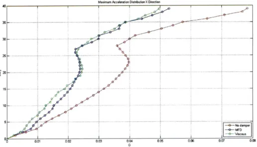
Maximvurm Acceleration Distribution X Direction

Fig. 21 Maximum acceleration profile for X direction

Floor Work X direction (kN*m)

5 27.7 7 32.3 9 31.5 11 46.6 13 45.8 15 52.8 17 50.0 19 59.8 21 54.1 23 72.2 25 62.6 27 46.2 29 37.6 31 34.0 33 22.1 (kN*m) 18.5 19.0 18.8 27.8 27.6 31.9 30.9 38.0 34.2 47.9 42.9 24.0 19.8 19.4 13.4

(31)

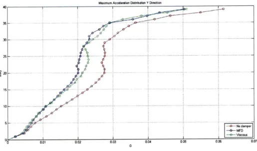
Maximum Acceleration Distnbution Y Direction

Fig. 22 Maximum acceleration profile for Y direction

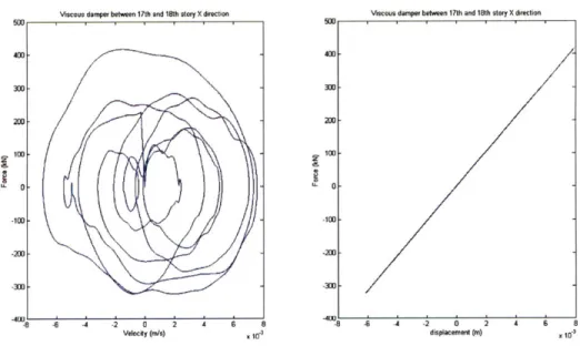
Viscous damper between 17th and 18th story X direction

8 -6 - 2 0 2

Velocity (m/s)

4 6

x i- . displacement (m)

(32)

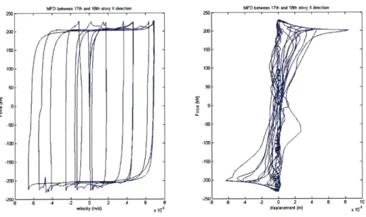
MFD between 17th and 18th story X direction

16o0 10

-150 -150

400t] -10

velocity (me) X 102 displacement (m) X 10

Fig. 24 MFD behavior between 17 and 18th floor X Direction

It is important to compare the maximum capacity for both devices. The viscous damper is exerting a maximum force of 400 kN (Fig. 23), while the MFD maximum capacity is half of this (Fig. 24). See in Fig. 21 and Fig. 22 that acceleration reduction is similar for both cases, but because of the control designed for the semi-active devices, much better efficiency in terms of maximum capacity of the device is obtained.

6.3. HEURISTIC STRATEGY

The way to remove devices for this first strategy consists in maintaining the spacing between MFDs. After checking the 2 floor spacing semi-active scheme behavior in section 6.2, devices are removed keeping a device spacing of 4, 6 and 8 stories. After every step, MFD maximum capacity is increased until behavior of the structure is similar to the viscous damper design. In addition to the increase of the device's maximum capacity,

Q

and R weight matrices are adapted to prevent MFDs working at full voltage (maximum friction) out of the hysteretic region (displacements close to zero). The reason to adapt MFDs behavior relies on the increase of accelerations in the system when MFD is working full voltage out of the maximum velocity area (regular friction device behavior).

(33)

6.3.1. MFD 600 KN EVERY 4 STORIES

accel. at 376 Flr.(m/s') 0.64 0.41 Response without dispi. at 3 7h Flr.(m/s) 0.40 0.28

dampers

Base Shear (kN) 9267 6140

accel. at 37h Flr.(m/s2) 0.43 0.35

Response with MFD displ. at 37* FIr.(m/s) 0.28 0.24

Base Shear (kN) 5652 4635

Table 8.Data obtained from the lumped model

Maximum Acceleation Distribution X Direction

Fig. 25 Maximum acceleration profile for X direction

(34)

Maximum Acceleratlion Distributlon Y Direction

Fig. 26 Maximum acceleration profile for Y direction

MFD between 17th and 18th story X direction MFD between 17th and 18th story X direction

400-400- 400 200 200 00 -20 -200-4-dI -400 S 8 -4 -2 2 A 6 8 -4 2 0 2 4 6 8

Wrecity (m/s) a- displacement (in)

Fig. 27 MFD behavior between 171h and 1₈th floor X Direction

Acceleration reduction for this first iteration is better than the reduction obtained for the viscous damper scheme (Fig. 25 and Fig. 26). The maximum capacity of the MFD is increased to 600 kN. In Fig. 27, velocity against MFD force is displayed on the left part. The controller shows a smooth behavior in the area of maximum velocities that prevents the device from generating high accelerations when the sign of the velocity changes (non-modified friction device).

(35)

6.3.2. MFD 1000 KN EVERY 6 STORIES

accel. at 37h Flr.(m/s2

) 0.64 0.41

Response without displ. at 37* Flr.(m/s) 0.40 0.28

dampers

Base Shear (kN) 9267 6140

accel. at 37* FIr.(m/s2) 0.43 0.33

Response with MFD displ. at 37th Flr.(m/s) 0.28 0.24

Base Shear (kN) 5644 4584

Maximum Acceleration Distwibution X Direction

(36)

Maximum Acceleration Distnbution Y Direction

Fig. 29 Data Maximum acceleration profile for Y direction

MFD between 17th and 18th story X direction

-locty-m/2 0 2 4 5 1

velocity (rrds)X o

MFD between 17th and 18th story X direction

displacement (M) X 103

Fig. 30 MFD behavior between 17th and 18th floor X Direction

Similar conclusions than those stated in section 6.3.1 could be provided for this iteration. However, there is an important difference to point out. Fig. 30 shows the behavior of the MFD between floors 1 7 th and 1 8 th for the X direction, the controller is be relaxed to get the

acceleration reduction desired, as a result of this, MFD behavior starts to seem like a viscous damper behavior. Hence, MFD starts to be inefficient (it does not work as it should) for this scheme.

...

(37)

6.3.3. MFD 2400 KN EVERY 8 STORIES

accel. at 37h Flr.(m/s2) 0.64 0.41

Response without displ. at 37' Flr.(m/s) 0.40 0.28

dampers

Base Shear (kN) 9267 6140

accel. at 370 Flr.(m/s2) 0.44 0.36

Response with MFD displ. at 37h Flr.(m/s) 0.28 0.25

Base Shear (kN) 5609 4533

Maxinum Acceleration Distribution X Direction

(38)

Maximum Acceleration Distibution Y Direction

Fig. 32. Data Maximum acceleration profile for Y direction

MFD between 17th and 18th story X direction

~8 -8 -d -2 0 2 4 t-6 -4 -2 0 2 4 velocity (m/s) 15W 1000 6 8 X 10 .3

MFD between 17th and 18th story X direction

-8 -6 4 -2 0 2 displacement (mn)

Fig. 33. MFD behavior between 17h and 18t' floor X Direction

Fig. 31 and Fig. 32 show that MFD between story _{2 4}th and _{2 5}th is problematic when trying

to reduce the accelerations. As a result, control is relaxed for this device in order to smooth the behavior. The same problem than 6.3.2 presented is observed in this iteration. Fig. 33 seems more a viscous behavior than a friction one as a result of the control relaxation.

1W

4 6 8

(39)

6.4.

STRATEGY BASED ON ENERGY DISSIPATION.

Keeping equal spacing between dampers seems a reasonable strategy. However, wind load is not uniformly distributed throughout the building. As a result, regular spacing may not be efficient in terms of wind excitation reduction. A second strategy is developed to decide which devices are going to be kept and which ones are going to be removed from the building. After analyzing the energy dissipated by every device (work done), those devices exerting smaller work into the structure are going to be removed gradually. At the same time,

Q

and R matrices are adapted to the new configuration and the device maximum capacity is increased to get similar acceleration reduction than the viscous damper original design.

6.4.1. Isr I TERA TION (400 KN MFD)

accel. at 3 7h FIr.(m/s

2

) 0.64 0.41

Response without displ. at 37' Flr.(m/s) 0.40 0.28

dampers

Base Shear (kN) 9267 6140

accel. at 37' Flr.(m/s2) 0.42 0.35

Response with MFD displ. at 37 Flr.(m/s) 0.27 0.24

Base Shear (kN) 5420 4257

(40)

Floor Work X direction (kN*m) Work Y direction (kN*m) 7 46.6 39.1 11 63.2 54.8 13 63.0 54.8 15 70.5 62.0 17 68.6 60.5 19 78.4 71.0 21 73.1 64.5 23 87.9 81.0 25 78.5 72.3 27 79.4 72.7 29 66.2 59.8 31 57.8 55.6

Table 12. Work done by the MFD's

Maximum A&teeation Disbtm~in X Directio

(41)

Moium Acceleration Distibution Y Direction

Fig. 35. Data Maximum acceleration profile for Y direction

MFD between 17th and 18th story X direction MFD between 17th and 18th story X direction

200 200 --lto - to 30 -0 -20 - -200 --300 - - -ID -300 -3D -8 -4 -2 0 2 A 6 8 :; - 2 0 2 6 a Velocity ("Vs) x displacerent (m) X 10"

Fig. 36. MFD behavior between 171h 18td 'h floor X Direction

In this first iteration, devices in stories 5, 9 and 33 are removed. MFD maximum capacity is 400 kN. The acceleration reduction for both directions is slightly better than the one obtained for viscous dampers (Fig. 34 and Fig. 35). The behavior of one of the devices is presented in Fig. 36. This plot shows a very smooth behavior when velocities are high while maintaining a friction nature when velocities are closer to zero.

(42)

6.4.2. 2ND ITERATION (400 KN MFD)

accel. at 37h Flr.(m/s2) 0.64 0.41

Response without displ. at 37h Flr.(m/s) 0.40 0.28

dampers

Base Shear (kN) 9267 6140

accel. at 37* Flr.(m/s2) 0.44 0.36

Response with MFD displ. at 37h Flr.(m/s) 0.29 0.24

Base Shear (kN) 5841 4476

Floor Work X direction (kN*m) Work Y direction (kN*m)

15 77.1 76.1 17 75.3 74.9 19 85.2 83.7 21 79.7 78.2 23 94.7 91.8 25 85.2 83.6 27 86.1 82.5 29 72.0 68.9 31 63.4 59.5

(43)

Maximum Acceleration Distribution X Direction

Fig. 37. Data Maximum acceleration profile for X direction

Maxunum Acceleraion Distnbution Y Direction

(44)

MFD between 17th and 18th story X direction

8 -6 -4 -2 0 2

velocity (m/s)

4 6 8

X 10,3 displacement (m) X 10

Fig. 39. MFD behavior between 17th ad 18th floor X Direction

Second iteration removes devices in stories 7, 11 and 13. MFD maximum capacity is keep as 400 kN. The acceleration reduction for both directions similar to the one obtained for viscous dampers (Fig. 34 Fig. 37 and Fig. 38). The behavior of one of the devices is presented in Fig. 36.

This behavior shows a very smooth behavior when velocities are high while maintaining a friction nature when velocities are closer to zero. The device in story 31 for the Y direction is critical in the design of this iteration (Fig. 38). The control is relaxed to avoid full voltage in the device when velocities are high.

6.4.3. 3RD ITERA TION (800 KN MFD)

accel. at 37" Flr.(m/s2) 0.64 0.41 Response without _{displ. at 37h Flr.(m/s)} _0.40 _0.28

dampers

Base Shear (kN) 9267 6140

accel. at 37* Flr.(m/s2₎

0.40 0.35

Response with MFD displ. at 37" Flr.(m/s) 0.25 0.24

Base Shear (kN) 5034 4550

(45)

Floor Work X direction (kN*m) 15 139.9 17 136.9 19 151.7 21 142.6 23 157.6 25 141.4 27 136.0 Work Y direction (kN*m) 83.5 79.8 96.0 84.6 115.0 101.7 107.3

Maximwn Acceteration Distsibtion X Direction

(46)

Maimum Acceleration Distnbrution Y Direction

Fig. 41. Data Maximum acceleration profile for Y direction

The third iteration involves removing devices in stories 29 and 31. In the design of the controllers for each device, MFD between floors 24 and 25 is the most critical (Fig. 40 and Fig. 41). Control is relaxed just for this device to generate a smooth behavior which reduces accelerations in the building.

MFD between 17th and 18th story X direction

8 -6 -4 -2 0 2

ietocity (nvs)

4 6

displacement (m) if'

Fig. 42. MFD behavior between 17th and 18th floor X Direction

(47)

Fig. 42 presents a strong friction behavior in the MFD while maintaining a smooth transition in the area of high velocities. In the right hand side, a very interesting hysteretic behavior is presented for MFD between 17 and 18 floor. Maximum capacity of the device is increased up to 800 kN.

6.4.4. 4TH ITERATION (800 KN MFD)

accel. at 37" Flr.(m/s2) 0.64 0.41

Response without displ. at 37h Flr.(m/s) 0.40 0.28

dampers

Base Shear (kN) 9267 6140

accel. at 37"' Flr.(m/s2) 0.43 0.37

Response with MFD displ. at 37*' Flr.(m/s) 0.28 0.25

Base Shear (kN) 5682 4412

Floor Work X direction (kN*m) Work Y direction (kN*m)

19 161.6 148.6

21 153.7 138.4

23 176.5 160.7

25 156.9 146.2

27 153.2 107.0

(48)

Maximum Acceleration Distribution X Direction

Fig. 43. Data Maximum acceleration profile for X direction

Devices in 15 and 17 stories are removed for this 4 th iteration (Table 18). MFDs installed in

21 and 25 floor are the most sensitive to acceleration performance. As a result, control is relaxed for both devices. If the last 3 stories are discarded, maximum acceleration of the building is the same for both viscous scheme and MFD scheme (Fig. 43 and Fig. 44). MFD maximum capacity is maintained to 800 kN and the behavior (Fig. 45) is similar to the one observed in the previous iteration.

Maximum Acceleration Distribution Y Direction

(49)

WD between 19th and 20th story X direction

-2001-41 .6 -4 -2 0 2 4 6 8 4.01 -0.00 -0.16 -.64 -0.02 0 0-002 0.004 0.006 0.00B 0.01

"Wcity (m/s) x i04 displacement (m)

Fig. 45. MFD behavior between 19th and 20' floor X Direction

6.4.5. 5TH ITER ATION (1500 KN MFD)

accel. at 37' Fr.(m/s2) 0.64 0.41

Response without displ. at 37' Flr.(m/s) _0.40 _0.28

dampers

Base Shear (kN) 9267 6140

accel. at 37' Flr.(m/s2) 0.45 0.37

Response with MFD displ. at 37' Flr.(m/s) 0.29 0.25

Base Shear (kN) 6102 4532

Floor Work X direction (kN*m) Work Y direction (kN*m)

19 280.7 212.3

23 213.9 233.6

25 170.7 172.2

(50)

Maximum Acceleration Distritbution X Direction

Fig. 46. Data Maximum acceleration profile for X direction

Maximum Acceleration Distrbution Y Direction

(51)

15m - 15W

-5M --W

-1XX - -1(

--15W - 15W

-- -S -4 - 0 2 4 6 s 15 -001 -0.A 0 0.S 1Ot 0.015

Vloct (t/s) X to- d1s0acemerd (m)

Fig. 48. MFD behavior between 1 9th and 2th floor X Direction

For the last iteration, MFDs in stories 21 and 27 are removed (Table 20). Device maximum capacity is chosen to be 1600 kN. Device controller for the 25 floor is critical in the design of the Y direction scheme. Hence, control has been relaxed fort this story. Building maximum accelerations obtained with this simple scheme are similar to the ones obtained for the initial viscous damper scheme (Fig. 46 and Fig. 47).

(52)

7. ECONOMIC EVALUATION

For the economic evaluation, a single viscous damper unit has a value of approximately $5,000 while MFD is estimated to be $15,000. However, bracing schemes have a great impact in the final total cost of the implementation. Hence, a basic economic evaluation has to compare every different solution previously presented. Final budgets are summarized in

Table 21 and Table 22.

Assuming a total cost of $1,000,000 for the current solution with viscous dampers and considering that toggle brace system (TBS) has a price 2 times bigger than the simple diagonal frame; unitary prices have been extrapolated for dampers and both bracing systems.

Due to the adaptability of the behavior for semi-active controlled systems. It has not been necessary to use toggle brace systems in the Y Direction. This fact has a direct impact on the final budget of the MFD's solutions because, as previously mentioned, this special bracing has a higher cost than the common diagonal bracing system.

After price for bracing units has been obtained and viscous damper bracing and connections are assumed to be designed to handle up to 300 kN, the cost of the rest of the bracing systems has been assumed to be linearly proportional to the respective device maximum capacity.

Number Price per Cost of the Price per Cost of Total Cost

of devices unit devices bracing the the

bracing

Viscous dampers X Direction 30 $5,000 $150,000 $7,778 $233,333 $1,000,000

Y Direction 30 $5,000 $150,000 $15,556 $466,667

MFD every 2 stories X Direction 30 $15,000 $450,000 $4,444 $133,333 $1,150,000

Y Direction 30 $15,000 $450,000 $4,444 $133,333

MFD every 4 stories X Direction 16 $15,000 $240,000 $13,333 $213,333 $900,000

Y Direction 16 $15,000 $240,000 $13,333 $213,333

MFD every 6 stories X Direction 10 $15,000 $150,000 $22,222 $222,222 $750,000

Y Direction 10 $15,000 $150,000 $22,222 $222,222

MFD every 8 stories X Direction 6 $15,000 $90,000 $53,333 $320,000 $820,000

Y Direction 6 $15,000 $90,000 $44,444 $266,667

(53)

Number Price per Cost of the Price per Cost of Total Cost

of devices unit devices bracing the the

bracing

Viscous dampers X Direction 30 $5,000 $150,000 $7,778 $233,333 $1,000,000

Y Direction 30 $5,000 $150,000 $15,556 $466,667 MFD 1st iteration X Direction 24 $15,000 $360,000 $8,889 $213,333 $1,150,000 Y Direction 24 $15,000 $360,000 $8,889 $213,333 MFD 2nd iteration X Direction 18 $15,000 $270,000 $8,889 $160,000 $860,000 Y Direction 18 $15,000 $270,000 $8,889 $160,000 MFD 3rd iteration X Direction 14 $15,000 $210,000 $17,778 $248,889 $920,000 Y Direction 14 $15,000 $210,000 $17,778 $248,889 MFD 4th iteration X Direction 10 $15,000 $150,000 $17,778 $177,778 $650,000 Y Direction 10 $15,000 $150,000 $17,778 $177,778 MFD 5th iteration X Direction 6 $15,000 $90,000 $40,000 $240,000 $660,000 Y Direction 6 $15,000 $90,000 $40,000 $240,000

Table 22. Economic evaluation based on the work measurement method

Considering economics and performance for the heuristic method, using MFD's either every 6 stories or 8 stories are the most sensible schemes to follow for the new implementation. However, when work done by every actuator has been considered to remove devices, much better economical solution has been achieved. The final budget for this implementation is reduced by a 45%.

Fig. 49. MFD final layout for X and Y direction.

Final solution consists in 2 MFD's per floor with maximum capacity of 800 kN located in stories 19,21,23,25 and 27 for every direction (X and Y).

(54)

8. CONCLUSIONS AND FURTHER STUDIES

Implementing MFD's with maximum capacity 200 kN every 2 stories has shown to be very efficient in terms of acceleration reduction under wind excitation. However, because of the assumed higher price of the devices in comparison to the common viscous damper, this solution would result more expensive than the current design.

After reducing the number of devices (every 4, 6 and 8 stories), same performance than wind viscous damper has been achieved. Because of the reduction in number of devices and bracing systems, more economical solutions than the current solution (viscous damper) are achieved. However, this heuristic method based on maintaining the same spacing between dampers has shown to be inefficient. Energy dissipation method has achieved much better solutions in terms of efficiency and economy.

Further studies would include the use of optimization method to select control matrices (see chapter 4). Besides, optimization tools could be used to allocate the MFDs throughout the building (work-based method) in order to optimize the final cost of the implementation. This thesis has used heuristic rules in order to reduce as much as possible the number of devices while maintaining the performance under wind excitations. However, improvement can be done in order to automate the process.

Finally, further studies have to be accomplished in terms of device control and structural behavior when undergoing seismic excitations.

(55)

9. REFERENCES

Abdellaoui, M. Study of a Modified Friction Device for the Control of Civil Structures.

Boston: MIT, 2010.

B.F. Spencer, Jr.and T.T. Soong. "New applications and development of active, semiactive and hybrid contorl techniques for seismic and non-seismic vibration in the USA."

International Post-SMiRT Conference Seminar on Seismic Isolation, Passive Energy Dissipation and Active Control of Vibration of Structures. Cheju, Korea, 1999.

Choi, S.B. and Lee, S.K. "A hysteresis model for the field-dependent damping force of a

magnetorheological damper." Journal of sound and vibration, 2001: 375-383. Connor, J.J. Introduction to Structural Motion Control. Boston: Prentice Hall, 2002.

content. answers. com.

http://content.answers.com/main/content/img/McGrawHill/Encyclopedia.

Dyke, S.J., B.F. Spencer Jr., M.K. Sain and J.D. Carlson. "Reduction, Modeling and Control of Magnetorheological Dampers for Seismic Response." 1996.

Housner, G.W. et al. "Structural control: past, present and future." Journal of Engineering

Mechanics, ASCE, 1997: 123:897-971.

Huang, R. J. McNamara and C. D. "An Efficient Damper System For High Rise Buildings." 2000.

Laflamme, S., Taylor, D., Abdellaoui Maane, M., and Connor, J. J. "Modified Friction Device for Control of Large-Scale Systems." In preparation, 2010.

Larrecq, G. Heating effects on Magnetorheological damper. Boston: MIT, 2010.

McNamara, R. and Taylor. "Fluid viscous dampers for high-rise buildings." the structural

design of tall and special buildings, 2003: 145-154.

McNamara, R. "Viscous-Damper with Motion Amplification Device."

www.taylordevicesindia.com. March 15, 2010. http://www.taylordevicesindia.com

(56)

APPENDIX

A

(VISCOUS DAMPER BRACING SCHEME)

Bottom Amplification Amplification Max stroke Msemice floor Cx(kN/m*s) Cy(kN/m*s) No dampers X No dampers Y factor X factorY wind X (kN) tkei

(kN) 5 52535 3502 2 2 0.70 7.16 721 2807 7 52535 3502 2 2 0.70 7.16 721 2807 9 52535 3502 2 2 0.70 7.16 721 2807 11 52535 3502 2 2 0.70 7.16 721 2807 13 52535 3502 2 2 0.70 7.16 721 2807 15 52535 3502 2 2 0.70 7.16 738 3056 17 52535 3502 2 2 0.70 7.16 738 3056 19 52535 3502 2 2 0.70 7.16 738 3056 21 52535 3502 2 2 0.70 7.16 738 3056 23 52535 3502 2 2 0.70 7.16 738 3056 25 52535 3502 2 2 0.70 7.16 627 2482 27 35024 1751 2 2 0.70 7.16 627 2482 29 35024 1751 2 2 0.70 7.16 627 2482 31 35024 1751 2 2 0.70 7.16 627 2482 33 35024 1751 2 2 0.70 7.16 627 2482

Bottom Max stroke Max stroke Cx total Cy total Max stroke Max stroke Max stroke Max stroke floor wind Y (kN) seismic Y (kN/m*s) (kN/m*s) wind X (kN) seismi X wind Y (kN) seism Y

flo wnY k) (kN) _________ ________ _____________ 5 160 712 73904 50165 604 2354 850 3778 7 160 712 73904 50165 604 2354 850 3778 9 160 712 73904 50165 604 2354 850 3778 It 160 712 73904 50165 604 2354 850 3778 13 160 712 73904 50165 604 2354 850 3778 15 151 712 73904 50165 619 2563 803 3778 17 151 712 73904 50165 619 2563 803 3778 19 151 712 73904 50165 619 2563 803 3778 21 151 712 73904 50165 619 2563 803 3778 23 151 712 73904 50165 619 2563 803 3778 25 71 587 73904 50165 526 2082 378 3117 27 71 587 49269 25082 526 2082 378 3117 29 71 587 49269 25082 526 2082 378 3117 31 71 587 49269 25082 526 2082 378 3117 33 71 587 49269 25082 526 2082 378 3117

Case study of a 39-story building : model verification and performance comparison with a semi-active device