HAL Id: hal-00221537
https://hal.archives-ouvertes.fr/hal-00221537
Submitted on 29 Jan 2008
HAL is a multi-disciplinary open access
archive for the deposit and dissemination of
sci-entific research documents, whether they are
pub-lished or not. The documents may come from
teaching and research institutions in France or
abroad, or from public or private research centers.
L’archive ouverte pluridisciplinaire HAL, est
destinée au dépôt et à la diffusion de documents
scientifiques de niveau recherche, publiés ou non,
émanant des établissements d’enseignement et de
recherche français ou étrangers, des laboratoires
publics ou privés.
Collective organization in an adaptative mixture of
experts
Vincent Vigneron, Christine Fuchen, Jean-Marc Martinez
To cite this version:
Vincent Vigneron, Christine Fuchen, Jean-Marc Martinez. Collective organization in an adaptative
mixture of experts. IEEE/SMC 18th international Conference Systems engineering (ICSE), Mar 1996,
Las-Vegas, United States. pp.00. �hal-00221537�
COLLECTIVE ORGANIZATION IN AN ADAPTIVE
MIXTURE OF EXPERTS
Vincent Vigneron1,2 and Christine Fuchen2 and Jean-Marc Martinez1
1 CEA de Saclay, DRN/ DMT/SERMA/LETR, 91191 Gif-sur-Yvette, France 2 CREL, 161, rue de versailles, 78180 Le Chesnay, France
Abstract. The use of multiple neural models have attracted much interest recently as pre-dictive models in system identification and control in the statistic and in the connectionist communities. In this paper, we shall restrict our attention to one particular form of density estimation called a mixture model. As well as providing powerful techniques for density tion, mixture models find important applications in techniques for conditional density estima-tion, in the technique of soft weight sharing and in mixture-of-experts model. By example, the hierarchical mixture-of-experts of Jacobs & Jordan have a powerful representational capacity and ability to handle with any multi-input multi-output mapping problem, yelding significantly faster training through the use of Expectation Maximisation algorithm. The general approach consists to divide the problem into a series of sub-problem and assign a set of ’experts’ to each sub-problem.
In this paper we design a new approach coupling EM algorithm (non-parametric) and Back-propagation rule (parametric) for a supervised/unsupervised segmentation of data originating from different unknown sources. We present this method as a feasible approach for learning any inverse mapping of causal systems, since Least-squares approach often leads to extremely poor performance if the image of an input is a non-convex region in the output.
But in contrast to mixture-of-experts architecture, the competitions depend on the relative per-formance of their experts-networks, not on the input. This reasonning leads to a somewhat Bayesian version of the ’decision’ by postulating a refinement of the data. the Bayesian con-text is presented as an alternative to the currently used frequency approach, which does not offer clear, compelling criterion for the design of statistical methods.
This approach is ’non-destructive’ in the sense that it does not force the data into a possibly inappropriate representation. As a simple illustration of this problem, we consider a problem of control of uranium enrichment by spectrometry-γ .
1
Introduction
Especially in the fields of classification and time series prediction, ANN have made substantial contributions. Of particular interest for modelling is their ability to describe the behaviour of any linear systems, proved by [?]. From a modeling point of view, a NN is a particular (often non-linear) parametrisation of a regression model for the system like y(x) = F (x, W). The device is capable to extract the underlying structure in the examples it was trained on and to ”generalise” from them.
But, since we have limited resources we would like to be able to use all our data to fit the model. Furthermore if the data originate from different sources, like many kinds of physical phenomena, direct approaches are likely to fail to represent the cancealled input-output relations.
[?] cited the non-causal approach as particularly relevant to map one-to-many relations, where the image of an input is a non-convex region in the output. There are three key ideas in our treatment. First, we demonstrate that reconstruction methods can be used to form the joint density P (x, y), to estimate, given a particular input x, the mixture representation for the vector function y = f (x). We show that these methods are preferable on grounds of convenience and accuracy and we believe they are more flexible than other recently proposed mixture of experts techniques. Secondly, we show that the mixture models approach allow much more subtle extraction of information from posterior distributions. Finally, we base our experiments and discussion on a model for mixtures that aim to provide a simple and generalisable way of being strongly informative about the mixing proportion parameters, even as an alternative to query learning.
2
Non-causal mixture of models
2.1 Background
We consider the case where the different input samples y(i) can be generated by a number n of
known functions fl, l= 1, . . . , n, i.e. y
(i)
l = fl(x(i), θl). The task then is to determine the functions
fl together with their respective contribution l(i) from a given data set X = {x(i), y(i)}Ni=1, where
x∈ <oand y ∈ <i. Since the functions are considered to be unknown, they have to be determined
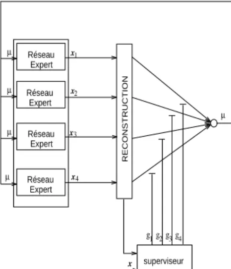
simultaneously (see Fig. 1), i.e. the correct attribution has to be found in an unsupervised manner.
Réseau Expert Réseau Expert Réseau Expert Réseau Expert x x x1 2 3 4 x x RECONSTRUCTION g1g g2 3g4 superviseur µ µ µ µ µ
Fig. 1.Competition-Cooperation in an inverse model. The modular approach presents three main advantages on the single BP models: it is able to model behavior, it learns faster than a global model and representation is easier to interpret : the modular architecture takes advantage of task decomposition, but the statistician must decide which variables to allocate to the networks.
In this strategy, the input data y(i) are physically segmented without prior knowledge about the
sources. Through these hard spatial constraints, we attribute at each input-output pair (yl(i), x(i))
a parcimonious model yl(i) = fl(x(i), θl). This segmentation assigns an expert-network to a single
geographical region or dimension of y. It is not necessary to rank the yl, to know which elements
are neighbors and which one are not. We show recently it is possible to take into account spacial contiguity constraints.
We therefore adapt the set of predictors fl, l= 1, . . . , n, by ”training”the netwoks on the
training-data set : we train the weights θl of network l by performing a gradient descent ∆θl ∝ −P∂C
(i) l
∂θl
on the squared costs Cl(i) = (fl(x(i)) − yl(i))2. Now, we can rewrite the output as the basic mixture
model for independant observations yl(i) as a mixture of inverse models :
x(i)∝
n
X
l=1
p(i)l gl(y(i)| θl), independantly for i = 1, . . . , N.
The objective of the analysis is inference about the unknown mixing proportions ”pl”. We postulate
a heterogeneous population from which our random sample is drawn (the objective of this modeling
step is not density estimation but fusion of data). The weighting coefficient p(i)l corresponds to
the relative probability for a contribution of network l and they are constrained to be Pnl=1pl =
1 and 0 < pl <1 for all l = 1, . . . , n. The gl(y(i) | θl) is the “contribution” (see section 2.2)of each
2.2 The inverse model
This section outlines the basic learning algorithm for finding the maximum likelihood parameters of the mixture model ([?,?]). [?] has shown that the EM algorithm is an alternate optimisation algorithm which considers the following decomposition of the (complete) likelihood :
`(Θ | X) = n X l=1 N X i=1 uillog {plgl(y(i) | µl, Σl)} − n X l=1 N X i=1 uillog uil, (1)
where Θ ≡ (u1, . . . , un; µ1, . . . , µn, Σ1, . . . , Σn) is the parameters vector. The EM algorithm is
an iterative method for maximising the former criterion. The intuition behind it is that if one had access to a ”hidden” random variable (here u) that indicated which data point was generated by which component, then the maximisation problem would decouple into a set of simple maximisations. `(Θ | X) can be maximised by iterating the following two steps :
E-step : uil= plˆgl(x (i)|µ l,Σl) P jpjˆgj(x(i)|µj,Σj) M-step : ˆµ(i)l = P iuilx(i) P iuil , Σl= P l P iuil(x(i)− ˆµl)(x(i)− ˆµl), ˆpl= P iuil n
using the Lagrange’s equation L = `(Θ | X) +Pnl=1λi(PNi=1uil− 1), where the λi are the Lagrange
coefficients corresponding to the constraintsPNi=1uil− 1 = 0, ∀i.
The E (Expectation) step computes the expected complete data log likelihood and the M
(Max-imisation) step finds the parameters that maximise this likelihood3. Convenient for calculation and
interpretation, the pl’s incorporate memory that is present in the process. This solution enables the
simultaneous determination of the numerical estimates of the a posteriori probability distribution
functions (pdfs) gland their uncertainties Σl.
An inverse problem entails the reliability of the inverse solution given the data set and the
class of models fl(. | θl) used to simulate the data. It arises in two rather distinct contexts ; the
first explore the classical frame of the bias-variance trade-off in the sense of [?]. In the second
context, the gl(. | θl)’s is thought of as a convenient parcimonious representation of a non-standard
density function, which is particularly well suited for any appropriate class of model, when a priori
information is available, i.e. by example the jacobian of each expert model ∂fl
∂x(i) (see [?]).
In this case, let both dx and be a finite shift in any model input towards the solution x∗, the
expected solution < x > and the variance σ2may be derived from :
< x >= Z x(i) pl ∂fl ∂xdx, and σ 2=Z x(i) p2l( ∂fl ∂x) 2dx− < x >2 . (2) The marginal pdf ∂fl
∂x may be interpreted as the bayesian prior of the parameter pl. For general
non-linear problems, its distribution cannot be predicted from a priori pdf or from the data pdf. In the following, we propose a complete procedure to estimate the output x of our inverse model :
3 maximising the log-likelihood is equivalent to minimising the non-equilibrium Helmholtz free-energy from
Algorithm
1. for a given y(i), compute x(i)0 = arg maxx(
P
l(fl(x
(i)) − y(i) l )2)
x being chosen in the training data set.
2. compute the mixing parameters pl following EM procedure
3. repeat x(i)= x(i)+ αP lpl ∂fl ∂x(i)δx (i) σ2= σ2+ αP l{p 2 l( ∂fl ∂x(i)) 2δx(i)− < x >2} until convergence.
Table 1.Inverse learning algorithm. The derivatives ∂fl
∂x(i) for each model l are calculated by backward
propagation starting from the output units.
One of the advantages of this model against the classical stochastic inverse techniques is that gaussian priors are rarely adequat to describe our a priori beliefs about the model parameters. A modified version of the algorithm 2.2 can be used for maximising also the criterion in Eq. 1. We
start by assuming that the outputs fl(xi) are distributed according to gaussians, i.e. pl∝ e−βCl. It
differs from previous work in the sense the competition between the expert-networks depends only on their relative performance and not on the input, in constrast to the mixture of experts architecture that uses an input-dependent gating-network ([?]). Bayes ’rule in this case gives for the weighting coefficients : ˆ pl= e−βCl P je−βCj (3) where the inverse temperature parameter β guarantees unambiguous competition. Eq. 3 is derived from Gas Theory of statistical Mechanics, called “Maximum Entropy” (see [?]). For β = 0, the
predictors equally share the same probability n1. Increasing β enforces the competition, thereby
driving the predictors to a specialisation (see [?]) when using algorithm 1. In the next section, we illustrate through case studies the general phenomenon of non-convex inverses in learning.
3
Applications and discussion
We start in this section by gathering exemples that tease out alternative explanations of the data, which would be difficult to discover by other approaches.
Uranium enrichment measurements As a first example of a non-convex problem, we present
prediction of Uranium enrichment from γ-spectra. These spectra are characterized by a vast number of highly correlated inputs. [?,?] showed that Calibration procedure and matrix effects can be avoided
by focusing the spectra analysis on a limited region, called KαX region. It is possible to learn such
Declared enrichment BP net Inverse Model 0,711% 0.700-0.720% 0.702-0.710% 1,416% 1.406-1.435% 1.406-1.416% 2,785% 2.762-2.799% 2.784-2.790% 5,111% 5.089-5.132% 5.112-5.136% 6,122% 6.117-6.133% 6.088-6.112% 9,548% 9.541-9.550% 9.542-9.552%
Table 2.Min-Max of calculated Enrichments with BP forward predictor and Inverse Model.
patterns, but with still an excessive number of weights and exhibiting a high non-convexity (see Fig. 2.c). This singular scheme referes extremely ill-posed learning problem [?] where an exemple consists of a very large input vector but where it is nevertheless the aim to learn and generalise froma relative number of examples.
Approaches to learning the inverse γ-spectrometric map by sampling the Kα region and directly
estimating a function ˜U = ˆf(x) where x ∈ <210 have met some success. Here, we propose an
alternative method where we use our density estimation technique to form a model of the enrichment predictor.
In Table 2, we compare the errors obtained on a backpropagation forward network using
cross-entropy error criterion to learn the direct mapping. It can be seen that little reaching error (about
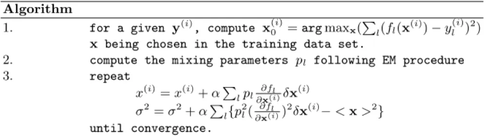
10−4) can be obtained. Fig. 2.b shows the mixing proportions pdf. when a (5,785%) spectrum is
presented to the inverse model. The credit assignement procedure on these 210 contributions is supervised (see algo. 1) to produce the final estimation.
Santa-Fe competition As an example for a high-dimensional chaotic system, we use the laser
data of the Santa-Fe Time series Prediction. The data are intensity measurements of a N H3 laser
believed to be in a chaotic state, exhibiting Lorentz-like dynamics.
-0.05 -0.04 -0.03 -0.02 -0.01 0 0.01 0.02 0.03 0.04 0.05 0.06 0 10 20 30 40 50 60 70 Number of spectrum Absolute error MLP 3-5-1 with normalized inputs
-0.05 -0.04 -0.03 -0.02 -0.01 0 0.01 0.02 0.03 0.04 0.05 0.06 0 10 20 30 40 50 60 70 Number of spectrum Absolute error MLP 3-5-1 with normalized inputs MNEX model 4.6 4.8 5 5.2 5.4 5.6 5.8 6 6.2 6.4 50 100 150 200 Number of output-node Estimation of Uranium Enrichment
0 50 100 150 05 1015 2025 3035 4045 -1 -0.5 0 0.5 1 Energy (MeV) Patterns
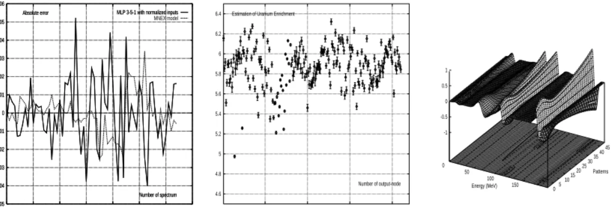
Fig. 2. (a) Absolute error in the enrichment estimation,(b) Example of enrichment value (at 5,785 %) predicted by the Mixture of Experts, c) 3-dimensions curves of KαX region on the whole data set
0 0.5 1 1.5 2 2.5 3 0 500 1000 1500 2000 0 5 10 15 20 25 3035 40 45 0 5 10 15 0 0.1 0.2 0.3 0.4 0.5 0.6 0.7 0.8 0.9 1
rank of the expert
Patterns counts 0 5 10 15 20 25 3035 40 45 0 5 10 15 0.005 0.01 0.015 0.02 0.025 0.03 0.035 0.04
rank of the expert
Patterns counts
Fig. 3.(a) plot of the Santa-Fe Time series Prediction, (b) mixing proportions for a test set with Maximum Entropy algorithm, (c) mixing proportions for a test set with EM algorithm
We limit our analysis to the prediction of a small numbers of step. 12,000 data points were learned by BP learning to map the inverse relation with 50 experts (we could have limited ourselves to a
dozen) using 200 iterations and iterating 3,000 times of the EM algorithmm, enough for approximate convergence. The density was then used to estimate the following 20 steps of the series. These outputs were then compared to the real values to obtain an error measure. This mean euclidean errors were
less than 10−1 for both inverse models. The localisation of multiple attribution of the experts (see
Fig. 3.b and 3.c) very informative of nature of the analysed phenomena. It is an interpretable, low dimensional projection of the data and often can lead to improved prediction performance.
4
conclusion
We have studied the feasability of applying ANNs to uranium enrichment measurement. The network
is shown to be able to calculate235U concentrations. Our results appear to be at the state of art in
automated quantifying methods for isotopes in a mixture of components.
Here, we have proposed an indirect approach to the non-convexity problem based on forming an internal model of the physical model. This method has been demonstrated as a reliable tool for dealing with few data under adverse conditions. The reconstruction part of the inverse algorithm can be viewed as linking adjacent predictions. It permits ready incorporation of results from the statistical literatures on missing data to yield flexible supervised and unsupervised learning architectures.