HAL Id: inria-00534333
https://hal.inria.fr/inria-00534333
Submitted on 10 Nov 2010
HAL is a multi-disciplinary open access
archive for the deposit and dissemination of
sci-entific research documents, whether they are
pub-lished or not. The documents may come from
teaching and research institutions in France or
abroad, or from public or private research centers.
L’archive ouverte pluridisciplinaire HAL, est
destinée au dépôt et à la diffusion de documents
scientifiques de niveau recherche, publiés ou non,
émanant des établissements d’enseignement et de
recherche français ou étrangers, des laboratoires
publics ou privés.
Multi-prover verification of floating-point programs
Ali Ayad, Claude Marché
To cite this version:
Ali Ayad, Claude Marché. Multi-prover verification of floating-point programs. Fifth International
Joint Conference on Automated Reasoning, Jul 2010, Edinburgh, United Kingdom. �inria-00534333�
Multi-Prover Verification of Floating-Point Programs
⋆ Ali Ayad1,3and Claude Marché2,31 CEA LIST, Software Safety Laboratory, F-91191 Gif-sur-Yvette 2
INRIA Saclay - Île-de-France, F-91893 Orsay
3
LRI, Univ. Paris-Sud, CNRS, F-91405 Orsay
Abstract. In the context of deductive program verification, supporting floating-point computations is tricky. We propose an expressive language to formally spec-ify behavioral properties of such programs. We give a first-order axiomatization of floating-point operations which allows to reduce verification to checking the validity of logic formulas, in a suitable form for a large class of provers includ-ing SMT solvers and interactive proof assistants. Experiments usinclud-ing the Frama-C platform for static analysis of C code are presented.
1
Introduction
Floating-point (FP for short) computations appear frequently in critical applications where a high level of confidence is sought: aeronautics, space flight, energy (nuclear plants), automotive, etc. There are numerous approaches for checking that a program runs as expected: testing, assertion checking at runtime, model checking, abstract in-terpretation, etc. Deductive verification techniques, originating from the landmark ap-proach of Floyd-Hoare logic, amounts to generating automatically logic formulas called
verification conditions(VCs for short), using techniques such as Dijkstra’s weakest
pre-condition calculus, so that validity of VCs entails soundness of the code with respect to its specification. The generated VCs are checked valid by theorem provers, hope-fully automatic ones. Complex behavioral properties of programs can be verified by deductive verification techniques, since these techniques usually come with expressive specification languages to specify the requirements. Nowadays, several implementa-tions of deductive verification approaches exist for standard programming languages, e.g., ESC-Java2 [12] and KeY [6] for Java, Spec# [3] for C#, VCC [29] and Frama-C [18] for Frama-C. In each of them, contracts (made of preconditions, postconditions, and several other kinds of annotations) are inserted into the program source text with spe-cific syntax, usually in a special form of comments that are ignored by compilers. The resulting annotation languages are called Behavioral Interface Specification Languages (BISL), e.g., JML [10] for Java, ACSL [5] for C.
To analyse accurary of FP computations, abstract interpretation-based techniques have shown quite successful on critical software. However, there are very few attempts
⋆
This work was supported by the French national projects: CerPan (Certification of numerical
programs, ANR-05-BLAN-0281-04), Hisseo (Static and dynamic analysis of floating-point
programs, Digiteo 09/2008-08/2011), and U3CAT (Unification of Critical C Code Analysis Techniques, ANR-09-ARPEGE)
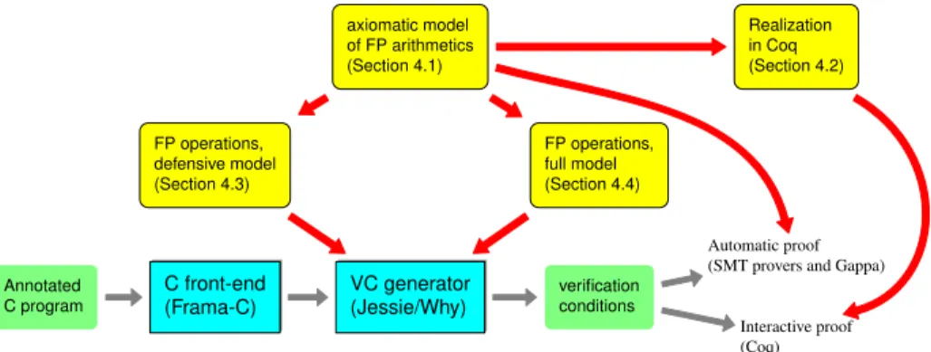
axiomatic model of FP arithmetics (Section 4.1) Realization in Coq (Section 4.2) FP operations, defensive model (Section 4.3) FP operations, full model (Section 4.4) Annotated C program C front-end (Frama-C) VC generator (Jessie/Why) verification conditions Automatic proof (SMT provers and Gappa)
Interactive proof (Coq)
Fig. 1.Architecture of our FP modeling
to provide ways to specify and to prove behavioral properties of FP programs in de-ductive verification systems like those above mentioned. This is difficult because FP computations are described operationally and have tricky behaviors as shown by Mon-niaux [25]. Consequently, it is hard to describe denotationally in a logic setting. A first proposal has been made in 2007 by Boldo and Filliâtre [7] for C code, using the Coq proof assistant [30] for discharging VCs. The approach presented in this paper is a follow-up of the Boldo-Filliâtre approach, which we extend in two main direc-tions: first a full support of IEEE-754 standard for FP computations, including special floating-point values ±∞ and NaN (Not-a-Number); and second the use of automatic theorem provers. Our contributions are the following:
– Additional constructs to specification languages for specifying behavioral proper-ties of FP computations. This is explained in Section 3.
– Modeling of FP computations by a first-order axiomatization, suitable for a large set of different theorem provers, and interpretation of annotated programs in this modeling (Section 4). There are two possible interpretations of FP operations in programs: a defensive version which forbids overflows and consequently apparition of special values (Section 4.3); and a full version which allows special values to occur (Section 4.4).
– Combination of several provers to discharge VCs (Section 5).
Our approach is implemented in the Frama-C [18] platform for static analysis of C code, and experiments performed with this platform are presented along this pa-per (see http://hisseo.saclay.inria.fr/gallery.html for other ex-amples). The lower part of Fig. 1 represents the current state of Frama-C, and the upper part presents the additions we make for dealing with FP computations.
2
The IEEE-754 Standard for Floating-Point Arithmetic
The IEEE-754 standard [1] defines an expected behavior of FP computations. It de-scribes binary and decimal formats to represent FP numbers, and specifies the
elemen-tary operations and the comparison operators on FP numbers. It explains when FP ex-ceptions occur, and introduces special values to represent signed infinities and NaNs. We summarize here the essential parts we need, see [19] for more details. In this paper we focus on the 32-bits (type float in C, Java) and 64-bits (type double) binary formats; adaptation to other formats is straightforward. Generally speaking, in any of these formats, an interpretation of the bit sequence under the form of a sign, a mantissa and an exponent is given, so that the set of FP numbers denote a finite subset of real numbers, called the set of representable numbers in that format.
For each of the basic operations (add, sub, mul, div, and also sqrt, fused-multiply-add, etc.) the standard requires that it acts as if it first computes a true real number, and then rounds it to a number representable in the chosen format, according to some
rounding mode. The standard defines five rounding modes: if a real number x lies
be-tween two consecutive representable FP numbers x1 and x2, then the rounding of x
is as follows. With mode Up (resp. Down), it is x2(resp. x1). With ToZero, it is x1if
x > 0 and x2if x < 0. With NearestAway and NearestEven, it is the closest to x among
x1and x2, and if x is exactly the middle of [x1, x2] then in the first case it is x2if x > 0
and x1if x < 0 ; whereas in the second case the one with even mantissa is chosen.
The standard defines three special values: −∞, +∞ and NaN. It also distinguishes between positive zero (+0) and negative zero (-0). These numbers should be treated both in the input and the output of the arithmetic operations as usual, e.g. (+∞) + (+∞) = (+∞), (+∞) + (−∞) = NaN, 1/(−∞) = −0, ±0/ ± 0 = NaN, etc.
IEEE-754 characterizes FP formats by describing their bit representation, but for formal reasoning on FP computations, it is better to consider a more abstract view of binary FP numbers: a FP number is a pair of integers (n, e), which denotes the real num-ber n × 2e, where n ∈ Z is the integer significand, and e ∈ Z is the exponent. For
ex-ample, in the 32-bit format, the real number 0.1 is approximated by40x1.99999Ap-4,
which can be denoted by the pair of integers (13421773, −27). Notice that this repre-sentation is not unique, since, e.g, (n, e) and (2n, e − 1) represent the same number. This set of pairs denote a superset of all FP numbers in any binary format. A suitable characterization of a given FP format f is provided by a triple (p, emin, emax) where p
is a positive integer called the precision of f, and eminand emaxare two integers which
define a range of exponents for f. A number x = n × 2eis representable in the format
f (f -representable for short) if n and e satisfy |n| < 2p and e
min≤ e ≤ emax. If
x is representable, its canonical representative is the pair (n, e) satisfying the property above for |n| maximal.5The characterization of the float format is (24, −149, 104)
and those of double is (53, −1074, 971). The largest f-representable number is (2p − 1)2emax. In order to express whether an operation overflows or not, we intro-duce a notion of unbounded representability and unbounded rounding: A FP
num-ber x = n × 2e is unbounded f-representable for format f = (p, e
min,, emax) if
|n| < 2p and e
min ≤ e. The unbounded f, m-rounding operation for given
for-mat f and rounding mode m maps any real number x to the closest (according to m) unbounded f-representable number. We denote that as roundf,m.
4C99 notation for hexadecimal FP literals: 0xhh.hhpdd, where h are hexadecimal digits and
dd is in decimal, denotes number hh.hh × 2dd
, e.g. 0x1.Fp-4 is (1 + 15/16) × 2−4. 5This definition allows a uniform treatment of normalized and denormalized numbers [1].
/*@ requires \abs(x) <= 1.0;
@ ensures \abs(\result − \exp(x)) <= 0x1p−4; */ double my_exp(double x) {
/*@ assert \abs(0.9890365552 + 1.130258690*x +
@ 0.5540440796*x*x − \exp(x)) <= 0x0.FFFFp−4; */
return 0.9890365552 + 1.130258690 * x + 0.5540440796 * x * x;
}
Fig. 2.Remez approximation of the exponential function
3
Behavioral Specifications of Floating-Point Programs
We propose extensions to specification languages in order to specify properties of FP programs. As a basis we consider classical first-order logic with built-in equality and arithmetic on both integer and real numbers. We assume also built-in symbols for stan-dard functions such as absolute value, exponential, trigonometric functions and such. Those are typically denoted with backslashes: \abs, \exp, etc. The core of the speci-fication language is made of a classical BISL (ACSL [5] in our examples) which allows function contracts (preconditions, postconditions, frame clauses, etc.), code annotations (code assertions, loop invariants, etc.) and data invariants.
To deal with FP properties, we first make important design choices. First, there is no FP arithmetic in the annotations: operators +, −, ∗, / denote operations on mathe-matical real numbers. Thus, there are neither rounding nor overflow that can occur in logic annotations. Second, in annotations any FP program variable, or more generally any C left-value of type float or double, denotes the real number it represents. The following example illustrates the impact of these choices.
Example 1. The C code of Fig. 2 is an implementation of the exponential function for
double precision FP numbers in interval [−1; 1], using a so-called Remez polynomial
approximationof degree 2.
The contract declared above the function contains a precondition (keyword requires) which states that this function is to be called only for values of x with |x| ≤ 1. The postcondition (keyword ensures) states that the returned value (\result) is close to the real exponential, the difference being not greater than 2−4.
The function body contains an assert clause, which specifies a property that holds at the corresponding program point. In that particular code, it states that the
expres-sion 0.9890365552 + 1.130258690x + 0.5540440796x2
− exp(x) evaluated as a real
number, hence without any rounding, is not greater than (1 − 2−16) × 2−4.
The intermediate assertion thus naturally specifies the method error, induced by the mathematical difference between the exponential function and the approximating polynomial; whereas the postcondition takes into account both the method error and the rounding errors added by FP computations.
So far we did not specify anything about the rounding mode in which programs are executed. In Java, or by default in C, the default rounding mode is NearestEven. In the C99 standard, there is a possibility for dynamically changing it using fesetround(). For efficiency issues, is not recommended to change it too often, so usually a program
//@ pragma allowOverflow //@ pragma roundingMode(Down)
typedef struct { double l, u; } interval;
/*@ type invariant is_interval(interval i) =
@ (\is_finite(i.l) || \is_minus_infinity(i.l)) &&
@ (\is_finite(i.u) || \is_plus_infinity(i.u)) ; */ /*@ predicate double_le_real(double x,real y) =
@ (\is_finite(x) && x <= y) || \is_minus_infinity(x);
@ predicate real_le_double(real x,double y) =
@ (\is_finite(y) && x <= y) || \is_plus_infinity(y);
@ predicate in_interval(real x,interval i) =
@ double_le_real(i.l,x) && real_le_double(x,i.u); */ /*@ ensures \forall real a,b;
@ in_interval(a,x) && in_interval(b,y) ==>
@ in_interval(a+b,\result); */
interval add(interval x, interval y) { interval z;
z.l = x.l + y.l; z.u = −(−x.u − y.u);
return z;
}
Fig. 3.Interval structure, its invariant, and addition of intervals
will run in a fixed rounding mode set once for all. To specify what is the expected rounding mode we choose to provide a special global declaration in the specification language: pragma roundingMode(value) ; where value is either one of the 5 IEEE modes, or ‘variable’, meaning that it can vary during execution. The default is thus pragma roundingMode(NearestEven). In the ‘variable’ case, a special ghost variable is available in annotations, to denote the current mode. Since the first case is the general one, we focus on it in this paper.
Usually, in a program involving FP computations, it is expected that special values for infinities and NaNs should never occur. For this reason we choose that by default, arithmetic overflow should be forbidden so that special values never occur. This first and default situation is called the defensive model: it amounts to check that no overflow occur for all FP operations. For programs where special values are indeed expected to appear, we provide another global declaration: pragma allowOverflow, to switch to the so-called full model. In that case, a set of additional predicates are provided: \is_finite, \is_infinite, \is_NaN are unary predicates to test whether an expression of type float or double is either finite, infinite or NaN. Additional shortcuts are provided, e.g. \is_plus_infinity, etc. (See [2] for details.)
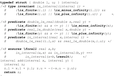
Example 2. Interval arithmetic aims at computing lower bounds and upper bounds of
real expressions. It is a typical example of a FP program that uses a specific rounding mode and makes use of infinite values.
An interval is a structure with two FP fields representing a lower and an upper bound. It represents the sets of all the real numbers between these bounds. Fig. 3 pro-vides a C implementation of such a structure, equipped with a data invariant [5] which states that the lower bound might be −∞ and the upper bound might be +∞. The two pragmas specify that overflows are expected and the Down rounding mode is in use. In the same figure, a behavioral specification for addition is specified via a predicate in_interval(x, i) stating that a real x belongs to an interval i. Notice the trick for computing the upper bound in Down mode, using negations.
Notice that since we choose a standard logic with total functions, usual caution must be taken [11]: a formula should mention the real value of some FP expression x only in contexts where \is_finite(x) is known to hold, such as in the definition of predicate double_le_real of Fig. 3 (similarly as one should mention 1/x only when x is known to be non-null).
4
Modeling FP Computations
We model FP programs and their annotations, in order to reduce soundness to proper VCs. We proceed in four steps, the ones schematized on the upper part of Fig. 1.
4.1 Axiomatization of FP Arithmetics
To remain prover-independent, we model FP numbers with abstract datatypes Single and Double (the support for more formats would amount to add new types). For each f among single and double, we introduce an observation function: value_f : f → R, supposed to denote the real number represented by a FP number (when it is finite). The largest f-representable number is introduced in our modelling by constants max_f : R defined as max_single = (224
− 1) × 2104and max_double = (253
− 1) × 2971.
The five IEEE rounding modes are naturally modelled by a concrete datatype
mode = Up | Down | ToZero | NearestAway | NearestEven. The function
roundf,m defined in Section 2 is introduced as an underspecified logic function
round_f : mode, R → R. Then, the following predicate indicates when the
round-ing does not overflow: no_overflow_f(m : mode, x : R) := |round_f(m, x)| ≤
max_f. For example, computing 10200
× 10200
in 64 bits overflows. In our
model, it is represented by round_double(NearestEven, 10200
× 10200
) which is
supposed to denote something close to 10400
. It exceeds max_Double, thus
no_overflow_Double(NearestEven, 10200
× 10200
) is false.
The rounding function round_f is not directly defined: we axiomatize it by some, incomplete, set of axioms. Here are two of them, useful in the examples of this paper: ∀m : mode; x, y : R,
|x| ≤ max_f ⇒ no_overflow_f (m, x) (1)
x ≤ y ⇒ round_f (m, x) ≤ round_f (m, y) (2)
In order to annotate FP programs that allow overflows and special values, we extend the above logical constructions with new types, predicates and functions. A natural
idea would be to introduce new constants to represent NaN, +∞, −∞. We do not do that for two reasons: first, there are several NaNs, and second, we want to keep the Single and Double types as abstract, equipped with observation functions, and not a mixed abstract/concrete representation with constants. Our proposal is thus to add two new observation functions, similar to value_f, to give the class of a float, either
finite, infinite or NaN; and its sign. We introduce two concrete types Float_class =
Finite | Infinite | NaN and Float_sign = Negative | Positive and additional functions class_f : f → Float_class and sign_f : f → Float_sign which indicate respectively the class and the sign of a FP number.
Additional predicates are defined to test if a FP number is finite, infinite, NaN, etc.: is_finite_f(x : f) := class_f(x) = Finite, and similar definitions for is_infinite_f, is_NaN_f, is_plus_infinity_f, is_minus_infinity_f, etc.
Comparison between two FP numbers is given by the predicates le_f, lt_f, eq_f, etc., e.g.
le_f(x : f, y : f) := (is_finite_f(x) ∧ is_finite_f(y) ∧ value_f(x) ≤ value_f(y)) ∨ (is_minus_infinity_f (x) ∧ ¬ is_NaN_f (y))
∨ (¬ is_NaN_f (x) ∧ is_plus_infinity_f (y))
We must constrain our model to ensure that the sign function is consistent with the sign of real numbers: whenever x represents a finite number, sign_f(x) should have the sign of value_f(x). This is achieved by the following definitions
same_sign_f(x : f, y : f) := sign_f(x) = sign_f(y) diff_sign_f(x : f, y : f) := sign_f(x) 6= sign_f(y) same_sign_real_f(x : R, y : f) :=
(x < 0 ∧ sign_f (y) = Negative) ∨ (x > 0 ∧ sign_f (y) = Positive) and an axiom: ∀x : f,
(is_finite_f (x) ∧ value_f (x) 6= 0) ⇒ same_sign_real_f (value_f (x), x) (3)
4.2 A Coq Realization of the Axiomatic Model
Our formalization of FP arithmetic is a first-order, axiomatic one. It is clearly under-specified and incomplete.
We realized this axiomatic model in the Coq proof assistant. This realization has two different goals. First, it allows us to prove the lemmas we added as axioms, thus providing an evidence that our axiomatization is consistent. Second, when dealing with a VC in Coq involving FP arithmetic, we can benefit from all the theorems proved in Coq about FP numbers. We build upon the Gappa [22] library which provides: (1) a definition of binary finite FP numbers: type float2 (a pair of integers as in section 2) together with a function float2R mapping (n, e) to the real n × 2e; (2) a complete
definition of the rounding function. Our realization amounts to declare types format, mode, Float_class and Float_sign as inductive types, and defines max_f by cases. The abstract types Single and Double are realized by Coq records whose fields are:
– The value_f field which is equal to (float2R genf); – The class_f field, of type Float_class;
– The sign_f field, of type Float_sign; – An invariant corresponding to axiom (3).
The last field is a noticeable point: it allows us to realize properly the finite_sign axiom above. Finally, the round_f operator is realized by the corresponding one in the Gappa library.
4.3 The Defensive Model of FP Computations
To model the effect of the basic FP operations, we now need to make an important assumption: we assume that both the compiler and the processor implement strict IEEE-754, that is any single operation acts as if it first computes a true real number, and then rounds the result to the chosen format, according to the rounding mode. For example, addition of FP numbers is addf,m(x, y) = roundf,m(x + y) for x, y non-special values,
where the + on the right is the mathematical addition of real numbers. This means in particular that addition overflows whenever the rounding overflows. We will discuss this assumption in Section 6.
We model FP operations in FP programs by abstract functions, using the Hoare-style notation f(x1, . . . , xn) : {P (x1, .., xn)}τ {Q(x1, .., xn, result)}, which
speci-fies that operation f expects arguments x1, . . . , xn satisfying P (this leads to a VC
at each call site) and returns a value r (denoted by keyword result) of type τ, such that Q(x1, .., xn, r) holds. In other words, in our modeling we do not say exactly how an
operation is performed, but only give its specification.
The defensive model must ensure that no overflows and no NaNs should ever occur. This can be done by proper preconditions to operations. For instance, division of FP numbers is modeled by an abstract function
div_f(m : mode, x : f, y : f) :
{ value_f (y) 6= 0 ∧ no_overflow_f (m, value_f (x)/value_f (y)) } f
{ value_f (result) = round_f (m, value_f (x)/value_f (y)) }
This reads as: the computation of a FP division requires to check that the divisor is not zero, and the result of the division in R does not overflow, and it returns a FP number in format f whose real value is the rounding of the real result. Other operations such that addition. subtraction, unary negation and multiplication are defined similarly, and also cast operations between float formats. The square root function is defined similarly, requiring that the argument is non-negative.
Notice that, for a given operation in a program, the expected format of the result is known at compile-time, by static typing. But on the contrary, it should be clari-fied what is the rounding mode to choose: we use whatever is declared by the pragma
roundingModein Section 3.
Particular care has to be taken for FP constant literals: they are not necessarily representable and they are rounded (usually at compile-time) to a FP number according
to a certain rounding direction (usually NearestEven). This is modeled by the following abstract function:
real_to_f(m : mode, x : R) :
{ no_overflow_f (m, x) } f { value_f (result) = round_f (m, x)}
This reads as: the real value of the literal must be able to be rounded without overflow, and then the result is its rounding.
4.4 The Full Model of FP Computations
The full model allows FP computations to overflow, and make use of special values: NaNs, infinities and signed zeros. Unlike for the defensive model, there are no pre-conditions on operations. We carefully interpret IEEE-754 informal specifications into postconditions taking all cases into account. Below is the complete specification for the multiplication (see [2] for other operations).
mul_f(m : mode, x : f, y : f) : { // no preconditions } f
{ ((is_NaN_f (x) ∨ is_NaN_f (y)) ⇒ is_NaN_f (result)) // NaNs arguments propagate to the result ∧ ((is_zero_f (x) ∧ is_infinite_f (y)) ⇒ is_NaN_f (result)) ∧ ((is_infinite_f (x) ∧ is_zero_f (y)) ⇒ is_NaN_f (result))
// zero times∞ gives NaN
∧ ((is_finite_f (x) ∧ is_infinite_f (y) ∧ value_f (x) 6= 0) ⇒ is_infinite_f (result)) ∧ ((is_infinite_f (x) ∧ is_finite_f (y) ∧ value_f (y) 6= 0) ⇒ is_infinite_f (result))
//∞ times non-zero finite gives ∞
∧ ((is_infinite_f (x) ∧ is_infinite_f (y)) ⇒ is_infinite_f (result))
//∞ times ∞ gives ∞
∧ ((is_finite_f (x) ∧ is_finite_f (y) ⇒
if no_overflow_f (m, value_f (x) × value_f (y))) then (is_finite_f (result)∧
value_f(result) = round_f(m, value_f(x) × value_f(y))) // finite times finite without overflow
else (overflow_value(m, result))) // finite times finite with overflow ∧ product_sign_f (result, x, y)
// in any case, sign of result is product of signs }
where
is_zero_f(x : f) := class_f(x) = Finite ∧ value_f(x) = 0 product_sign_f(z : f, x : f, y : f) :=
(same_sign_f (x, y) ⇒ sign_f (z) = Positive)∧ (diff_sign_f (x, y) ⇒ sign_f (z) = Negative)
overflow_value(m : mode, x : f) := (m = Down ⇒
(sign_f (x) = Negative ⇒ is_infinite_f (x))∧
(sign_f (x) = Positive ⇒ is_finite_f (x) ∧ value_f (x) = max_f )) ∧ (m = Up ⇒
(sign_f (x) = Positive ⇒ is_infinite_f (x))∧
(sign_f (x) = Negative ⇒ is_finite_f (x) ∧ value_f (x) = −max_f )) ∧(m = ToZero ⇒ is_finite_f (x)∧
(sign_f (x) = Negative ⇒ value_f (x) = −max_f (f ))∧ (sign_f (x) = Positive ⇒ value_f (x) = max_f (f ))) ∧(m = NearestAway ∨ m = NearestEven ⇒ is_infinite_f (x))
The auxiliary predicate overflow_value specifies the result of FP operations, in case the real result overflows, depending on its sign and the rounding mode. The predicate product_sign_f encodes the usual rule for the sign of a product. Those are reused for other operations.
5
Discharging Proof Obligations
Our aim is to support as many theorem provers as possible. However, we must consider provers that are able to understand first-order logic with integer and real arithmetic. Suitable automatic provers are those of the SMT-family (Satisfiability Modulo Theo-ries) which support first-order quantification, such as Z3 [15], CVC3 [4], Yices [16], Alt-Ergo [13]. Due to the high expressiveness of the logic, these provers are necessarily incomplete. Hence we may also use interactive theorem provers, such as Coq and PVS. Additionally, recall that our modeling involves an uninterpreted rounding function round_f. The Gappa tool [23] is an automatic prover, which specifically handles for-mulas made of equalities and inequalities over expressions involving real constants, arithmetic operations, and the round_f operator. But unlike SMT provers, Gappa does not handle quantifiers.
All the provers mentioned above are available as back-ends for the Frama-C envi-ronment and its Jessie/Why plugin [17]. Our experiments are conducted with those.
Example 3 (Example 1 continued).The VCs for our Remez approximation of
exponen-tial are the following:
– 3 VCs for the representability of constants 0.9890365552; 1.130258690
and 0.5540440796 in double format. These are proved by Gappa and by SMT solvers. SMT solvers make use of the axiom (1) on round_f.
– 5 VCs for checking that the three multiplications and the two additions do not overflow. These are automatically proved by Gappa. This demonstrates the power of Gappa to check non-overflow of FP computations in practice.
– 1 VC for the validity of the post-condition. This is also proved by Gappa, as a consequence of the assertion. In other words, whenever Gappa is given the method error, it is able to add the rounding error to deduce the total error.
– 1 VC for the validity of the assertion stating the method error. This is not proved by any automatic prover. It corresponds to the VC:
∀x : Double, |value_Double(x)| ≤ 1.0 ⇒
|0.9890365552 + 1.130258690 × value_Double(x) + 0.5540440796× value_Double(x) ∗ value_Double(x) − exp(value_Double(x))|
≤ (1 − 2−16) × 2−4
Indeed, value_Double(x) is just an arbitrary real number here, and that formula is a pure real arithmetic formula. It is expected that no automatic prover proves it since they do not know anything about the exp function. However, this VC can be proved valid using the Coq proof assistant, in a very simple way (2 lines of proof script to write) thanks to its interval tactic [23], which is able to bound mathematical expressions using interval arithmetic.
Example 4 (Interval example continued). Although the code for interval addition
(Fig. 3) is very simple, it was not proved by automatic provers. We started an interactive proof in Coq, and saw that the proof was complex because it involved a large amount of different cases to distinguish, depending on whether interval bounds are finite or in-finite, and whether an overflow occurs or not. Nevertheless, no case was difficult, and we found that the important property that automatic provers were missing was that for any format f and real x: round_f(Down, x) ≤ x, which can be proved correct using our Coq realization. Adding this property in our axiomatization of round_f allows to perform the verification with SMT solvers.
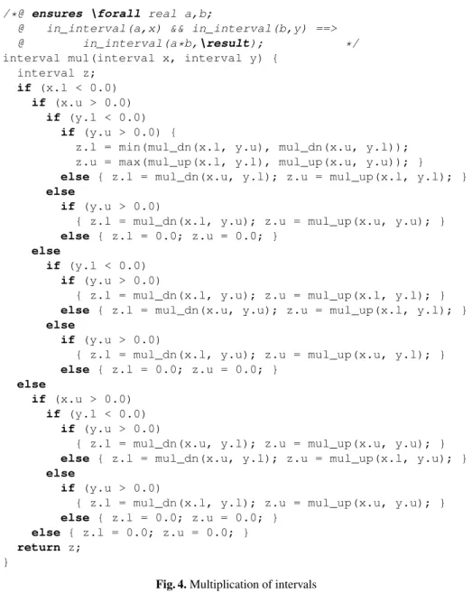
Example 5 (Interval multiplication).To go further, we proved also the multiplication
of intervals. Its code is given in Fig. 4. Notice the large number of branches. This code calls some auxiliary functions on intervals from Fig. 5. This was difficult to verify. First, we had to find proper contracts for the auxiliary functions: see the preconditions about signs for mul_up and mul_dn. Second, the number of cases is definitely larger than for addition: we got a total of 140 VCs, where each of them has a complex propositional structure, leading to consider a large number of subcases. By investigating in Coq the VCs which were not proved automatically, we were able to discover that SMT solvers were missing a few lemmas related to multiplication, e.g for all reals x, y, z and t:
(0 ≤ x ≤ z ∧ 0 ≤ y ≤ t) ⇒ x × y ≤ z × t (0 ≤ z ≤ x ∧ y ≤ t ∧ y < 0) ⇒ x × y ≤ z × t and similar others.
The Z3 prover is able to validate all VCs except one (the first post-condition of mul_up). This is done in around 45s on a 3GHz CPU (each VCs is solved within 0.5s), whereas the remaining VC cannot be proved with a 2 minutes time limit. Fortunately, the CVC3 prover is able to solve the remaining VC, but misses 7 other VCs. CVC3 needs a similar amount of time. What is important here is the very good efficiency of SMT solvers, for dealing with all the cases coming from the complex propositional structures of VCs.
/*@ ensures \forall real a,b;
@ in_interval(a,x) && in_interval(b,y) ==>
@ in_interval(a*b,\result); */
interval mul(interval x, interval y) { interval z;
if (x.l < 0.0) if (x.u > 0.0)
if (y.l < 0.0) if (y.u > 0.0) {
z.l = min(mul_dn(x.l, y.u), mul_dn(x.u, y.l)); z.u = max(mul_up(x.l, y.l), mul_up(x.u, y.u)); }
else { z.l = mul_dn(x.u, y.l); z.u = mul_up(x.l, y.l); } else
if (y.u > 0.0)
{ z.l = mul_dn(x.l, y.u); z.u = mul_up(x.u, y.u); }
else { z.l = 0.0; z.u = 0.0; } else
if (y.l < 0.0) if (y.u > 0.0)
{ z.l = mul_dn(x.l, y.u); z.u = mul_up(x.l, y.l); }
else { z.l = mul_dn(x.u, y.u); z.u = mul_up(x.l, y.l); } else
if (y.u > 0.0)
{ z.l = mul_dn(x.l, y.u); z.u = mul_up(x.u, y.l); }
else { z.l = 0.0; z.u = 0.0; } else
if (x.u > 0.0) if (y.l < 0.0)
if (y.u > 0.0)
{ z.l = mul_dn(x.u, y.l); z.u = mul_up(x.u, y.u); }
else { z.l = mul_dn(x.u, y.l); z.u = mul_up(x.l, y.u); } else
if (y.u > 0.0)
{ z.l = mul_dn(x.l, y.l); z.u = mul_up(x.u, y.u); }
else { z.l = 0.0; z.u = 0.0; } else { z.l = 0.0; z.u = 0.0; } return z;
}
Fig. 4.Multiplication of intervals
6
Related Works and Perspectives
There exist several formalizations of FP arithmetic in various proof environments: two variants in Coq [14, 22] and one in PVS [24] exclude special values; one in ACL2 [27] and one in HOL-light [20] also deal with special values. Compared to those, our purely first-order axiomatization has the clear disadvantage of being incomplete, but has the advantage of allowing use of off-the-shelf automatic theorem provers. Our approach
al-/*@ requires !\is_NaN(x) && !\is_NaN(y);
@ ensures \le_float(\result,x) && \le_float(\result,y);
@ ensures \eq_float(\result,x) || \eq_float(\result,y); */ double min(double x, double y) { return x < y ? x : y; } /*@ requires !\is_NaN(x) && !\is_NaN(y);
@ ensures \le_float(x,\result) && \le_float(y,\result);
@ ensures \eq_float(\result,x) || \eq_float(\result,y); */ double max(double x, double y) { return x > y ? x : y; } /*@ requires !\is_NaN(x) && !\is_NaN(y);
@ requires (\is_infinite(x) || \is_infinite(y))
@ ==> \sign(x) != \sign(y);
@ requires (\is_infinite(x) && \is_finite(y)) ==> y != 0.0;
@ requires (\is_infinite(y) && \is_finite(x)) ==> x != 0.0;
@ ensures double_le_real(\result,x*y);
@ ensures (\is_infinite(x) || \is_infinite(y)) ==>
@ \is_minus_infinity(\result); */
double mul_dn(double x, double y) { return x*y; } /*@ requires !\is_NaN(x) && !\is_NaN(y);
@ requires (\is_infinite(x) || \is_infinite(y))
@ ==> \sign(x) == \sign(y);
@ requires (\is_infinite(x) && \is_finite(y)) ==> y != 0.0;
@ requires (\is_infinite(y) && \is_finite(x)) ==> x != 0.0;
@ ensures real_le_double(x * y,\result);
@ ensures (\is_infinite(x) || \is_infinite(y)) ==>
@ \is_plus_infinity(\result); */
double mul_up(double x, double y) { return −(x*(−y)); } Fig. 5.Auxiliary functions on intervals
lows to incorporate FP reasoning in environments for program verification for general-purpose programming languages like C or Java.
In 2006, Leavens [21] described some pitfalls when trying to incorporate FP special values and specifically NaN values in a BISL like JML for Java. In its approach, FP numbers, rounding and such also appear in annotations, which cause several issues and traps for specifiers. We argue that our approach, using instead real numbers in annotations, solves these kind of problems.
In 2006, Reeber & Sawada [28] used the ACL2 system together with a automated tool to verify a FP multiplier unit. Although their goal is at a significantly different con-cern (hardware verification instead of software behavioral properties) it is interesting to remark that they came to a similar conclusion, that using interactive proving alone is not practicable, but incorporating an automatic tool is successful.
In Section 5, we have seen that we needed both SMT solvers, Gappa for reasoning about rounding, and interactive proving to prove all VCs. Improving cooperation of provers is an interesting perspective, e.g. like in the Jahob verification tool for Java [31] which selects the prover to call depending on the class of goal (but does not support FP).
Turning the Gappa techniques for FP into some specific built-in theory for SMT solvers should be considered. Integrating SMT solvers into interactive proving systems is also potentially very useful: possibility of calling Z3 and Vampyre from Isabelle/HOL has been experimented recently, and similar integration in Coq is in progress.
Another future work is to deal with programs, where FP computations do not strictly respect the IEEE standard, due to transformations made at compile-time (reorganization of expression order, use of fused multiply-add instructions) ; or at runtime by using extra precision (e.g., 80 bits FP precision in 387 processors) on intermediate calculations [8]. Discovering the proper annotations (e.g. contract for mul_up above) is essential for successful deductive verification. Another interesting future work is to automatically in-fer annotations, for example using abstract interpretation techniques [26] or abstraction refinement [9], to assist this task.
Acknowledgements We thank G. Melquiond for his help in the use of the Gappa tool, the FP-specific Coq tactics, and more generally for his suggestions about the approach presented here.
References
1. IEEE standard for floating-point arithmetic. Technical report, 2008. http://dx.doi. org/10.1109/IEEESTD.2008.4610935.
2. A. Ayad and C. Marché. Behavioral properties of floating-point programs. Hisseo publica-tions, 2009. http://hisseo.saclay.inria.fr/ayad09.pdf.
3. M. Barnett, K. R. M. Leino, and W. Schulte. The Spec# Programming System: An Overview. In Construction and Analysis of Safe, Secure, and Interoperable Smart Devices (CASSIS’04), volume 3362 of LNCS, pages 49–69. Springer, 2004.
4. C. Barrett and C. Tinelli. CVC3. In W. Damm and H. Hermanns, editors, Proceedings of the
19th International Conference on Computer Aided Verification (CAV’07), Berlin, Germany, LNCS. Springer, 2007.
5. P. Baudin, J.-C. Filliâtre, C. Marché, B. Monate, Y. Moy, and V. Prevosto. ACSL: ANSI/ISO
C Specification Language, 2008. http://frama-c.cea.fr/acsl.html.
6. B. Beckert, R. Hähnle, and P. H. Schmitt, editors. Verification of Object-Oriented Software:
The KeY Approach, volume 4334 of LNCS. Springer, 2007.
7. S. Boldo and J.-C. Filliâtre. Formal Verification of Floating-Point Programs. In 18th IEEE
In-ternational Symposium on Computer Arithmetic, pages 187–194, Montpellier, France, 2007.
8. S. Boldo and T. M. T. Nguyen. Hardware-independent proofs of numerical programs. In
Pro-ceedings of the Second NASA Formal Methods Symposium, NASA Conference Publication,
Washington D.C., USA, Apr. 2010.
9. A. Brillout, D. Kroening, and T. Wahl. Mixed abstractions for floating-point arithmetic. In
FMCAD’09, pages 69–76. IEEE, 2009.
10. L. Burdy, Y. Cheon, D. Cok, M. Ernst, J. Kiniry, G. T. Leavens, K. R. M. Leino, and E. Poll. An overview of JML tools and applications. International Journal on Software Tools for
Technology Transfer, 2004.
11. P. Chalin. Reassessing JML’s logical foundation. In Proceedings of the 7th Workshop on
Formal Techniques for Java-like Programs (FTfJP’05), Glasgow, Scotland, July 2005. 12. D. R. Cok and J. R. Kiniry. ESC/Java2 implementation notes. Technical
re-port, may 2007. http://secure.ucd.ie/products/opensource/ESCJava2/ ESCTools/docs/Escjava2-ImplementationNotes.pdf.
13. S. Conchon, E. Contejean, J. Kanig, and S. Lescuyer. CC(X): Semantical combination of congruence closure with solvable theories. In Proceedings of the 5th International Workshop
SMT’2007, volume 198-2 of ENTCS, pages 51–69. Elsevier Science Publishers, 2008. 14. M. Daumas, L. Rideau, and L. Théry. A generic library for floating-point numbers and its
application to exact computing. In Theorem Proving in Higher Order Logics (TPHOLs’01), volume 2152 of LNCS, pages 169+, 2001.
15. L. de Moura and N. Bjørner. Z3, an efficient SMT solver. http://research. microsoft.com/projects/z3/.
16. B. Dutertre and L. de Moura. The Yices SMT solver. available at http://yices.csl. sri.com/tool-paper.pdf, 2006.
17. J.-C. Filliâtre and C. Marché. The Why/Krakatoa/Caduceus platform for deductive pro-gram verification. In W. Damm and H. Hermanns, editors, 19th International Conference
CAV’2007, volume 4590 of LNCS, pages 173–177, Berlin, Germany, July 2007. Springer.
18. The Frama-C platform, 2008. http://www.frama-c.cea.fr/.
19. D. Goldberg. What every computer scientist should know about floating-point arithmetic.
ACM Computing Surveys, 23(1):5–48, 1991.
20. J. Harrison. Floating point verification in HOL Light: The exponential function. Formal
Methods in System Design, 16(3):271–305, 2000.
21. G. Leavens. Not a number of floating point problems. Journal of Object Technology, 5(2):75– 83, 2006.
22. G. Melquiond. Floating-point arithmetic in the Coq system. In Proceedings of the 8th
Conference on Real Numbers and Computers, pages 93–102, Santiago de Compostela, Spain,
2008. http://gappa.gforge.inria.fr/.
23. G. Melquiond. Proving bounds on real-valued functions with computations. In Proceedings
of the 4th IJCAR, volume 5195 of LNAI, pages 2–17, 2008. http://www.lri.fr/
~melquion/soft/coq-interval/.
24. P. S. Miner. Defining the IEEE-854 floating-point standard in PVS. Technical Memorandum 110167, NASA Langley, 1995.
25. D. Monniaux. The pitfalls of verifying floating-point computations. ACM Transactions on
Programming Languages and Systems, 30(3):12, May 2008.
26. D. Monniaux. Automatic modular abstractions for linear constraints. In 36th ACM
Sympo-sium POPL 2009, pages 140–151, 2009.
27. J. S. Moore, T. Lynch, and M. Kaufmann. A mechanically checked proof of the correctness of the kernel of the AMD5k86 floating-point division algorithm. IEEE Transactions on
Computers, 47(9):913–926, 1998.
28. E. Reeber and J. Sawada. Combining ACL2 and an automated verification tool to verify a multiplier. In Sixth International Workshop on the ACL2 Theorem Prover and its
Applica-tions, pages 63–70. ACM, 2006.
29. W. Schulte, S. Xia, J. Smans, and F. Piessens. A glimpse of a verifying C compiler. http: //www.cs.ru.nl/~tews/cv07/cv07-smans.pdf.
30. The Coq Development Team. The Coq Proof Assistant Reference Manual – Version V8.2, 2008. http://coq.inria.fr.
31. K. Zee, V. Kuncak, and M. Rinard. Full functional verification of linked data structures. In