HAL Id: hal-00720265
https://hal.inria.fr/hal-00720265
Submitted on 24 Jul 2012HAL is a multi-disciplinary open access
archive for the deposit and dissemination of sci-entific research documents, whether they are pub-lished or not. The documents may come from teaching and research institutions in France or
L’archive ouverte pluridisciplinaire HAL, est destinée au dépôt et à la diffusion de documents scientifiques de niveau recherche, publiés ou non, émanant des établissements d’enseignement et de recherche français ou étrangers, des laboratoires
association studies with neuroimaging data
Benoit da Mota, Vincent Frouin, Edouard Duchesnay, Soizic Laguitton, Gaël
Varoquaux, Jean-Baptiste Poline, Bertrand Thirion
To cite this version:
Benoit da Mota, Vincent Frouin, Edouard Duchesnay, Soizic Laguitton, Gaël Varoquaux, et al.. A fast computational framework for genome-wide association studies with neuroimaging data. 20th In-ternational Conference on Computational Statistics (COMPSTAT 2012), Aug 2012, Limassol, Cyprus. �hal-00720265�
genome-wide association studies
with neuroimaging data
Benoit Da Mota, Parietal Team, MSR-INRIA joint centre, benoit.da [email protected] Vincent Frouin, CEA, DSV, I2BM, Neurospin, [email protected]
Edouard Duchesnay, CEA, DSV, I2BM, Neurospin, [email protected]
Soizic Laguitton, CEA, DSV, I2BM, Neurospin, CATI, [email protected] Ga¨el Varoquaux, Parietal Team, INRIA Saclay, [email protected]
Jean-Bapiste Poline, CEA, DSV, I2BM, Neurospin, [email protected] Bertrand Thirion, Parietal Team, INRIA Saclay, [email protected]
Abstract. In the last few years, it has become possible to acquire high-dimensional neu-roimaging and genetic data on relatively large cohorts of subjects, which provides novel means to understand the large between-subject variability observed in brain organization. Genetic association studies aim at unveiling correlations between the genetic variants and the numer-ous phenotypes extracted from brain images and thus face a dire multiple comparisons issue. While these statistics can be accumulated across the brain volume for the sake of sensitivity, the significance of the resulting summary statistics can only be assessed through permutations. Fortunately, the increase of computational power can be exploited, but this requires designing new parallel algorithms. The MapReduce framework coupled with efficient algorithms permits to deliver a scalable analysis tool that deals with high-dimensional data and thousands of per-mutations in a few hours. On a real functional MRI dataset, this tool shows promising results with a genetic variant that survives the very strict correction for multiple testing.
Keywords. Bio-statistics, Neuroimaging, Genetics, Genome-Wide Brain-Wide Analysis, Mass Univariate Linear Model, Permutation Tests, Spatial Model, Cluster-Level Inference.
1
Introduction
The integration of genetics information with neuroimaging data promises to significantly im-prove our understanding of both normal and pathological variability of brain organization. It should lead to the development of biomarkers and in the future personalized medicine. Among
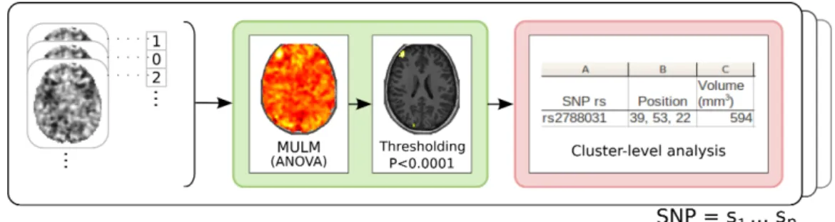
Figure 1. Sketch of the cluster-level analysis. Colors of the boxes are references to tasks of our framework described in Figure 2 (MULM: Mass Univariate Linear Model ).
other important steps, this endeavor requires the development of adapted statistical methods to extract significant correlations between the highly heterogeneous variables provided by genotyp-ing and brain imaggenotyp-ing, and the development of the software components that will permit large computation to be done.
In current settings, neuroimaging-genetic datasets consist of a set of i) genotyping measure-ments on genetic variables, such as Single Nucleotide Polymorphisms (SNPs) that represent a large amount of the genetic between-subject variability, on the one hand, and ii) quantitative level at given locations (voxels) in three-dimensional images, that represent either the amount of functional activation in response to a certain task or an anatomical feature (e.g. the density of grey matter in this brain region). The standard approach for voxelwise Genome-Wide As-sociation Studies (vGWAS) is the Mass Univariate Linear Model (MULM) [10], that considers each (SNP, voxel) pair independently and tests the significance of the correlation between these traits. With 50k voxels and 500k SNP, the number of comparisons reaches to 25 billions, thus controling the Type 1 error rate at p < .05 with Bonferroni family-wise error rate (FWER) correction implies a selecting only p-value smaller than 2.10−12. However, genetic markers are not independent, such that the genotype of two close SNP on the same chromosome tend to be highly correlated, due to the cross over phenomenom during cell meiosis (this is called link-age desiquilibrium or LD). It implies that Bonferroni correction yields conservative thresholds, at the expense of statistical power. This approach is therefore weakly sensitive, as it detects only extreme peaks in the statistics and fails to uncover smaller, but spatially extended, effects. Analytical corrections have been proposed to take into account thee correlations between these variables, but they yield only small improvement, and their theoretical validity needs to be further assessed [18]. In the brain imaging domain, cluster-level analysis techniques have been proposed [19], where the statistical test deals with the size of supra-threshold regions, for a pre-defined detection threshold (see Figure 1). In the absence of accurate statistical model of the largest cluster size under the null hypothesis, these approaches require permutations to control the significance of the decision statistic. Permutations also automatically adapt the threshold to the amount of correlation among genetics variables.
To assess the statistical significance with a sufficient accuracy, up to 104
permutations are needed. Traditional computational architectures that rely on popular analysis softwares (Plink or SPM) cannot manage this load in a reasonable amount of time. The size of our problem makes the computational load a primary concern and many parameters should be taken into account to design efficient and scalable parallel procedures. Working in a distributed context
Figure 2. Overview of the Map-reduce framework for the neuroimaging-genetics univariate model.
is necessary to deal with the memory and computational loads, and yields specific optimization strategies. For instance, with permutation tests the most natural way of spliting the problem consists in distributing the computations according to permutations. But this causes inefficient access to data, because each sub-problem needs all the data. With such natural data parallel application, the main task is to choose how to split the problem into smaller sub-problems to minimize computation and communication overhead. For the first time, we propose an efficient framework that can manage cluster-based inference in a vGWAS.
In Section 2, we describe our framework to distribute efficiently the computation on large infrastructures, then present the optimization of the sequential algorithm. Experimental results on simulated and real data are presented in Section 3.
2
Methods : the computational framework
The mass-univariate statistical analysis of neuroimaging genetics is clearly an embarrassingly parallel problem, nevertheless this can be easily split into smaller tasks. A good computational framework has to rely on an adapted workflow and each sub-task has to be optimized for the sake of efficiency. Although these two steps must be addressed jointly in practical settings, to simplify the presentation we first describe the workflow and then the optimization of the algorithms.
The distributed algorithm
The MapReduce framework [3, 4] seems the most natural approach to handle this problem and can easily harnest large grids. The Map step yields statistical scores between each (SNP, voxel) pair and the reduce step consists in collecting all results to compute statistic distribution and corrected p-values. Scores are p-values obtained with an Ordinary Least Square (OLS) regres-sion. The key point is to create subtasks in a way that minimises inputs/outputs (I/O); in particular, requiring all the data for each subtask is a waste of ressources. By essence, permuta-tions imply computapermuta-tions on the same data after shuffling. So the permutation procedure should be embedded in the inner loop, such that all permutations are done on the same node for a given dataset. The problem can be split in two other directions: genomic and/or brain data, where each one can have up to 106
variables. We choose to split in both dimensions for performance and memory reasons. As cluster-based inference requires all scores per SNP in all the brain, we introduce in the MapReduce framework a new task, the combine task, that combines several map results to do the cluster-based computation. The combine task is used to pre-compute statistic distributions and drastically reduces the amount of data transfered between the combine and reduce phase. Figure 2 gives an overview of our framework.
Optimization of the sequential algorithm
Algorithm 2.1 Fit the model Y = xβ + Zγ + ǫ for all x in X = [x1, .., xq] and get a score for
each pair (SNP, voxel)
Require: The data Y, the X and Z regressor matrices if first regression then
Zw ← (ZTZ)−1/2Z {whitening}
Ynorm ← Y ∆1−1 with ∆1= diag(kYik, i = 1 . . . p) {p number of voxels}
Xnorm ← X∆2−1 with ∆2= diag(kxik, i = 1 . . . q) {q number of SNPs}
RY |Z ← Ynorm− Zwβˆ1 with ˆβ1= ZwTYnorm {residuals}
RX|Z ← Xnorm− Zwβˆ2 with ˆβ2 = ZwTXnorm {residuals}
cache← Zw, RY |Z, RX|Z else Zw, RY |Z, RX|Z ← cache end if ˆ β ← RX|ZTRY |Z ˆ
γ ← ZwTRY |Z {for Freedman and Lane approximation [16]}
F-scores ∝ 1 βˆ2 − ˆβ2−ˆΓ2 with ˆΓ 2 = Pr i=1 ˆ
γi2 {r = number of confounding variables} return ˆβ, F-scores
The map step is the most demanding in computation time (> 99% in our final implemen-tation) and thus has to be optimized in priority. For one (SNP, voxel) pair, we want to fit the model y = xβ + Zγ + ǫ, where y is a vector of observations (i.e. values for a voxel), x a vector of number of minor alleles for a SNP, Z a matrix of confounding variables (age, sex, acquisition center, ...) and the intercept. We propose the Algorithm 2.1, that optimizes this step based on the following observations :
• To fit the model, the vector y is implied in only one product, so y should be a matrix such that several voxels are regressed during the same operation.
• The fit operation is dominated by a costly pseudo-inverse of the design matrix. If the regressors in the design matrix are orthonormal, the computation is simplified to a product, with a much lower cost.
• The effects of the confounding variables are first removed from y and x, then the regression is done on the residuals (Ry|Z and Rx|Z). With this strategy, the fit of the last regression is a scalar product so that we can fit the regression of several voxels and SNPs in the same Matrix product.
• Some properties are insensitive to permutations and the results can be cached to speed up regressions on permuted data. For instance, the norm of a column does not change after a permutation on row, orthogonality is preserved too.
• Permutations can be done on the residuals. For this purpose, we use de method called per-mutation under the reduced model by Freedman and Lane [16], shown as the best possible approximation of the true model [1]. Further speed up can be achieved using the method proposed by Kennedy [20], however this approximation is not precise enough because we need very good accuracy far in the tail of the distribution.
The same level of detail cannot be handled depending on whether few genes or the whole genome were considered. In our setting, with the univariate model, keeping all the associations represents more than 2 petabytes in double precision (8 × 104
× 5.105
× 5.104
). For this reason, we store only, in single precision, p-values lower than a threshold, called sparsity threshold. This reduction saves a large amount of time because of bandwidth and space economy. The aggregation of scores per SNP represents the other most significant fraction of the execution time of the mapper because norms of large matrices (number of voxels × number of SNPs) are involved. Normalizing the matrices greatly simplifies the calculation. We also take care of computational/hardware sources of optimization: CPU cache issues, data access pattern, I/O bottlenecks. For instance, if we profile the execution of the standard mass univariate linear model, we can observe that computing over phenotypes or explanatory variables one by one is inefficient. Matrix-based operations should thus be sued instead of vector-based operations. Our Python code uses the Numpy/Scipy scientific libraries, which rely on standard and optimized linear algebra libraries (Atlas or MKL) that are several order of magnitude faster than naive code.
3
Results
We present three types of results. As we aim to provide a fast whole brain whole genome ex-ploratory tool, we evaluate the performances of our serial procedure and distributed framework. Then, we illustrate the interest of our approach on simulated data with known ground truth. Finally, we present our results on the IMAGEN study [8].
Procedure GWAS time in sec. Speed in assoc.
per sec. Speedup 1 Speedup 2
Plink v1.05 in [10] ∼540 8.30 × 10² 1 -Plink v1.06 ∼2 2.24 × 10⁵ 270 1 Our mapper 0.081 5.50 × 10⁶ 6667 25
Table 1. Comparison of execution time and speed of Plink and our mapper. Speedup 1 is the speedup against the performance reported in [10], while Speedup 2 is the speedup against Plink with our settings.
Performance evaluation of the procedure
To the best of our knowledge, there is only one voxel wise Brain-wide Genome-wide (BWGW) association study [10] that reports computational performances. The authors used a modified version of the Plink software [14] to manage the size of the outputs. Plink is a popular whole genome association analysis toolset designed to be computationally efficient. In the domain of neuroscience, the most popular tool to do such study is SPM, but is far less efficient. Although SPM can be scripted, it is not designed for efficiency in studies with many external covariates, such as neuroimaging-genetics studies, so we do not report its performance.
As our approach is very different from Plink, we calculate the speed of a procedure in (SNP, voxel) associations per second with fixed number of samples, i.e. 740 to match the cohort size in the previous study [10]. We use Plink (v1.06) and determine an optimistic time for a GWAS at around 2 seconds. Our experiments run on one core of a 2 × Intel(R) Xeon(R) CPU X5660 (6 cores) @ 2.8GHz with 24GB of memory. Our mapper runs with the academic version of the Entought Python Distribution (EPD 7.2-2-rh5 64 bits), with the MKL as linear algebra library with OpenMP parallelization disabled. The results are reported in Table 1. Compared to this study, we achieved the computations thousands times faster. In a more realistic comparison based on our target application, we evaluate the speedup to approximately 25. Note that Plink gives much more detailed results and a part of the speedup of our mapper comes from a reduction of the output. Indeed, the additional results are not required by our application.
To illustrate the scalability of our Map-Reduce procedure, we execute the whole framework on our cluster: 20 nodes; each one is a 2 × Intel(R) Xeon(R) CPU X5650 (6 cores) @ 2.67GHz with 48GB of memory, connected with Gigabit Ethernet LAN; all files were written on the NFS storage filesystem; the code was executed in the same Python environment as previously described; the workflow is described and submitted with the soma-workflow software[13]. Soma-workflow framework enables i) to describe a set of independent tasks that are executed following an execution graph and ii) to execute the code by submitting the graph to classical queueing systems operating on the cluster. We report in Figure 3 the result of an execution with almost all the 240 cores available during all the run. The workflow is composed by 3,000 mappers, 300 combiners and 1 reducer tasks. The mappers represent 99.5% of the total of serial computation time, and the combiners 0.5%. We achieve a speedup of 227 comparing to the serial time. We can see in Figure 3 that after five hours, we use only half of the cores, but all the unused cores are available for other users. There are two easy ways to improve this speedup. First, if we can rely on a given number of cores, we can generate an optimal workflow. For instance, we can split to have 2,400 mappers, 240 combiners and 1 reducer with 240 cores. Second, we can split the problem into smaller pieces to decrease the time of the mappers. We do not explore further this possibilities, because performance is sufficient and we focus on experimental results.
Nb of voxels : 51,792 Nb of SNPs : 418,669 Nb of samples : 740 Nb of permutations : 1,000
Nb of tasks : 3, 000 + 300 + 1 Theoritical serial time : 53 days 13h 45min Total time : 5h 40min
Max cores : 240
Speedup: 227
Figure 3. Setting and execution of the Map-Reduce algorithm on the cluster.
Results on simulated data
We simulate functional Magnetic Resonance Images (fMRI) from real genetic data obtained from the Imagen database [8]. We use the number of minor alleles for each SNP and we assume an additive genetic model. Ten random SNPs produce an effect in a spherical brain region, centered at random positions in the standard space, then intersected with the support of grey matter using a mask computed for the Imagen dataset (see below). We add i.i.d. Gaussian noise, smoothed spatially with a Gaussian kernel (σ = 3mm), to model other variability sources. The effect size and the Signal-to-Noise Ratio (SNR) can vary across simulations.
To assess our approach, ten different datasets were generated and were ran on our framework with P=1,000 permutations to compute the different distributions under the null hypothesis. The sparsity threshold was set to raw p-value ≤ 10−4, which means that mappers only reports
raw p-values that meets this constraint. Four decision statistics were used to control the FWER : • The min(p) statistic assesses the significance of an association between a SNP and a voxel. • The total volume statistic is defined as the number of voxels for which the correlation with the SNP is smaller than the sparsity threshold. It assesses whether the volume of the brain associated with an SNP is significant.
• The P− log10(p) statistic is close from the total volume statistic with the difference
that the volume of each voxel is weighted by the strength of the association expressed in log (p-value).
• The cluster volume statistic is defined as the largest number of spatially connected vox-els for which the correlation with the SNP is smaller than the sparsity threshold. The difference with the total volume statistic is the connectivity constraint.
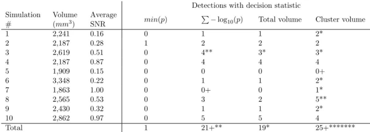
For each statistic considered, we report in Table 2 the number of detected SNPs, near detections (i.e. the causal SNP is not detected but a neighbour SNP in LD is) and unique detections (i.e. only one method detect the causal SNP).
With no surprise, the min(p) statistic only detects an extreme peak and is far less sensitive than the other methods due to the 2 × 10¹⁰
tests performed. Its main advantage is that of not requiring permutations when used with the Bonferonni FWER correction. Other methods do not consider each SN P × voxel association separately, but assess the impact of an SNP on the whole brain and require permutations to estimate the associated statistical significance. These three methods are more sensitive because the number of tests drops to 5 × 10⁵
Detections with decision statistic Simulation # Volume (mm3 ) Average SNR min(p) P− log
10(p) Total volume Cluster volume
1 2,241 0.16 0 1 1 2* 2 2,187 0.28 1 2 2 2 3 2,619 0.51 0 4** 3* 3* 4 2,187 0.87 0 4 4 4 5 1,909 0.15 0 0 0 0+ 6 3,348 0.22 0 1 1 2* 7 1,863 1.00 0 0+ 0 1* 8 2,565 0.53 0 3 2 5** 9 2,430 0.32 0 1 1 2* 10 2,862 0.97 0 5 5 4 Total 1 21+** 19* 25+*******
Table 2. Results on the simulated datasets with type I errors control by a FWER ≤ 0.05. The volume is the volume of the effect to find and average SNR is the mean of the signal-to-noise ratio for this effect. Numbers indicates how many causal SNPs were detected, a ’∗’ indicates an unique detection, and a ’+’ indicates a near detection.
of our simulation, i.e. the spatially extended effect of an SNP is in only one region, the cluster-based analysis gives the best results with the detection of 25 of the 100 causal SNP, including 7 unique detections. The total volume and the sum statistics give close, slightly poorer results and detect some causal SNP missed by the cluster-based analysis. These two methods are probably best suited for detecting spatially extended effects in two regions or more. On real data, all these methods could be complementary depending on the shape and intensity of the effects. A closer look at the results shows that effects with high SNR but confined to small volumes are difficult to detect with all statistics. The volume of the effect is comparable with that of smooth noise areas, so that the SNR level is critical for the sake of detections.
Results on IMAGEN data
We used data from Imagen, a large functional neuroimaging database [8] containing fMRI as-sociated with 99 different contrast images in more than 1,500 subjects. The dataset is built on the first batch of subjects of the study. Regarding the functional neuroimaging data, the faces protocol [23] was used, with the [angry faces - neutral] contrast (i.e. the difference between watching angry faces or neutral faces).
Imaging phenotype. Standard preprocessing, including slice timing correction, spike and motion correction, temporal detrending (functional data), and spatial normalization (anatomical and functional data), were performed using the SPM8 software and its default parameters; functional images were resampled at 3mm resolution. Obvious outliers detected using simple rules such as large registration or segmentation errors or very large motion parameters were removed after this step. The [angry faces - neutral] contrast was obtained using a standard linear model, based on the convolution of the time course of the experimental conditions with the canonical hemodynamic reponse function, together with standard high-pass filtering procedure and temporally auto-regressive noise model. The estimation of the model parameters was carried out using the SPM8 software. A mask of the grey matter was built by avergaing and thresholding the individual grey matter probability maps. Subjects with too many missing data (imaging
or genetic) or not marked as good in the quality check were discarded. An outliers detection (method described in [17]) was ran and we eliminate 10% of the most outlier subjects.
Genotype. We keep only SNPs with less than 2% missing data. All the remaining missing data were replaced by the median over the subjects for the corresponding variable. The age, the sex and the acquisition center were taken as confounding variables.
The final dataset contains 453 subjects, 51,792 voxels, 494,480 SNPs and 10 confounding variables. Our Map-Reduce framework was run on the this dataset with P=10,000 permutations to assess statistical significance with a good degree of confidence. The sparsity threshold was set to raw p-value ≤ 10−4. This choice permits to limit the intermediary results to 200GB, an amount that the NFS filesystem can manage. The workflow takes approximately 50 hours on the previously described 240 cores cluster, for a theoretical serial time around 475 days. We report in Figure 4 only 4 SNPs with the lowest corrected p-values; the genes close to the supra-threshold SNPs are identified with the UCSC genome browser [15]. We also provide views of the effects in the brain for this 4 SNPs.
Only one SNP, rs1021831, is associated with a corrected p-value ≤ 0.05 for 3 of the 4 decision statistics to voxels in the visual cortex. This SNP is in an intergenic region, far from any gene. The second best SNP, rs436760, is only detected by the min(p) statistic with corr. p = 0.14 and it is located in the promoter region of the ADAM28 gene. Associated voxels are in the superior prefrontal cortex. The third SNP, rs7778308, is associated with corr. p ≤ 0.23 for the total volume and sum statistics and is located in the GRM8 gene. Associated voxels are near the intraparietal sulcus. The last SNP, rs8065460, was found by the cluster-size statistic with corr. p = 0.29 and it is located in the promoter region of the ANKFN1 gene. Associated voxels are in the precuneus.
To fulfil the annotation of our findings we used GeneValorization [2] and search if the found genes were studied in the context of addictions or mental diseases: GRM8 has been associated with alcohol dependence [6], anxiety [5, 11], attention deficit hyperactivity disorder [9], heroin addiction [22] and schizophrenia [11, 26]. These preliminary results should be taken with caution and need to be reproduced.
4
Discussion and conclusion
Cluster-based inference promises large gains in terms of sensitivity to better detect associations between the brain and genetics. But this method requires permutations to assess the statistical significance of results and thus it has a prohibitive cost with popular analysis softwares. In this paper, we present an efficient and scalable framework that can deal with such a computational burden and that we used to provide a realistic assessment of the statistical power of our approach on simulations, which had never been done before. Our results on simulated data highlight the potential of our method and we provide interesting preliminary results on real data, including one association that passes the significance threshold after correction for multiple testing. As far as we know, this is the first time that such a result was obtained in a voxelwise genome-wide association study, although it needs to be reproduced to be considered meaningful.
Our method could be improved following two directions, addressing some drawbacks of the cluster based inference. First, the threshold on the statistical maps is arbitrarily chosen and
Chr SNP min. corr. p P− log10 corr. p
Volume
corr. p Cluster corr. p Gene p-value (mm3 ) (mm3 ) (±50kb) 12q24.32 rs1021831 6.49 × 10⁻⁹ 1 2,804 0.05 15,390 0.05 14,391 0.01 8p21.2 rs436760 7.99 × 10⁻¹² 0.14 768 1 4,050 1 1,404 1 ADAM28 7q31.33 rs7778308 1.22 × 10⁻⁸ 1 2,134 0.22 11,934 0.23 3,375 1 GRM8 17q22 rs8065460 7.08 × 10⁻⁹ 1 1,698 0.54 8,721 0.75 7,263 0.29 ANKFN1 rs1021831 L R y=-82 x=-3 L R z=1 rs7778308 L R y=-61 x=-31 L R z=45 rs436760 L R y=24 x=-42 L R z=30 rs8065460 L R y=-59 x=2 L R z=52
Figure 4. Results of the vGWAS on IMAGEN dataset with the differents methods and corre-sponding brain localizations. A gene is in bold typeface if the SNP is located in the gene.
has a major impact on the significant clusters found. Methods to avoid this problem exists, like the threshold-free cluster enhancement presented in [25]. Second, image noise is not uniformly smooth, so that larger clusters are expected in smoother areas. Introducing non-stationarity in our simulation would make it more realistic. Methods to limits this problem also exists [24]. These are promising ways to improve the sensitivity of cluster-based inference.
Another gain in sensitivity could be provided by multivariate models in which the joint variability of several genetic variables is considered simultaneously but would have an impact on computational speed. Such models are thought to be more powerful [27, 7, 12, 21], because they can express more complex relationships than simple pairwise association models. The cost of unitary fit becomes much higher (due to non-smooth optimization problems and various cross-validation loops needed to optimize the parameters), and moreover, permutation testing is necessary to assess the statistical significance of the results of such procedures. These methods require many efforts to be tractable for our problem on the algorithmic and implementation side as well as in the design of adapted and dimension reduction schemes.
Acknowledgement
Support of this study was provided by the IMAGEN project, which receives research funding from the European Community’s Sixth Framework Program (LSHM-CT-2007-037286) and coor-dinated project ADAMS (242257) as well as the UK-NIHR-Biomedical Research Centre Mental Health, the MRC-Addiction Research Cluster Genomic Biomarkers, and the MRC program grant Developmental pathways into adolescent substance abuse (93558). This research was also supported by the German Ministry of Education and Research (BMBF grant # 01EV0711).
This manuscript reflects only the author’s views and the Community is not liable for any use that may be made of the information contained therein.
Bibliography
[1] M. J. Anderson and J. Robinson. Permutation tests for linear models. Australian and New Zealand Journal of Statistics, (43):75–88, 2001.
[2] B. Brancotte, A. Biton, I. Bernard-Pierrot, F.Radvanyi, F. Reyal, and S. Cohen-Boulakia. Gene list significance at-a-glance with GeneValorization. Bioinformatics, 27(8):1187–1189, Apr 2011.
[3] C-T. Chu, S. K. Kim, Y-A. Lin, Y. Yu, G. R. Bradski, A. Y. Ng, and K. Olukotun. Map-reduce for machine learning on multicore. In B. Sch¨olkopf, J. C. Platt, and T. Hoffman, editors, NIPS, pages 281–288. MIT Press, 2006.
[4] J. Dean and S. Ghemawat. MapReduce: simplified data processing on large clusters. Com-mun. ACM, 51(1):107–113, January 2008.
[5] R. M. Duvoisin, L. Villasana, M. J. Davis, D. G. Winder, and J. Raber. Opposing roles of mGluR8 in measures of anxiety involving non-social and social challenges. Behav Brain Res, 221(1):50–54, Aug 2011.
[6] A. C. H. Chen et al. Association of single nucleotide polymorphisms in a glutamate receptor gene (GRM8) with theta power of event-related oscillations and alcohol dependence. Am J Med Genet B Neuropsychiatr Genet, 150B(3):359–368, Apr 2009.
[7] F. Bunea et al. Penalized least squares regression methods and applications to neuroimag-ing. Neuroimage, 55(4):1519–1527, Apr 2011.
[8] G. Schumann et al. The IMAGEN study: reinforcement-related behaviour in normal brain function and psychopathology. Mol Psychiatry, 15(12):1128–1139, Dec 2010.
[9] J. Elia et al. Genome-wide copy number variation study associates metabotropic glutamate receptor gene networks with attention deficit hyperactivity disorder. Nat Genet, 44(1):78– 84, Jan 2012.
[10] J. L. Stein et al. Voxelwise genome-wide association study (vGWAS). Neuroimage, 53(3):1160–1174, Nov 2010.
[11] M. J. Robbins et al. Evaluation of the mGlu8 receptor as a putative therapeutic target in schizophrenia. Brain Res, 1152:215–227, Jun 2007.
[12] O. Kohannim et al. Boosting power to detect genetic associations in imaging using multi-locus, genome-wide scans and ridge regression. In Biomedical Imaging: From Nano to Macro, 2011 IEEE International Symposium on, pages 1855 –1859, 30 2011-april 2 2011. [13] S. Laguitton et al. Soma-workflow: a unified and simple interface to parallel computing
resources. In MICCAI Workshop on High Performance and Distributed Computing for Medical Imaging, Toronto, Sep. 2011.
[14] S. Purcell et al. PLINK: a tool set for whole-genome association and population-based linkage analyses. Am J Hum Genet, 81(3):559–575, Sep 2007.
[15] W. J. Kent et al. The human genome browser at UCSC. Genome Res, 12(6):996–1006, Jun 2002.
[16] D. Freedman and D. Lane. A nonstochastic interpretation of reported significance levels. Journal of Business & Economic Statistics, 1(4):292–98, 1983.
[17] V. Fritsch, G. Varoquaux, B. Thyreau, J-B. Poline, and B. Thirion. Detecting outlying subjects in high-dimensional neuroimaging datasets with regularized minimum covariance determinant. Med Image Comput Comput Assist Interv, 14(Pt 3):264–271, 2011.
[18] X. Gao, L. C. Becker, D. M. Becker, J. D. Starmer, and M. A. Province. Avoiding the high Bonferroni penalty in genome-wide association studies. Genet Epidemiol, 34(1):100–105, Jan 2010.
[19] S. Hayasaka and T. E. Nichols. Validating cluster size inference: random field and permu-tation methods. Neuroimage, 20(4):2343–2356, Dec 2003.
[20] P. E. Kennedy. Randomization tests in econometrics. Journal of Business & Economic Statistics, 13(1):85–94, 1995.
[21] N. Meinshausen and P.B¨uhlmann. Stability selection. Journal of the Royal Statistical Society: Series B (Statistical Methodology), 72(4):417–473, 2010.
[22] D. A. Nielsen, F. Ji, V. Yuferov, A. Ho, A. Chen, O. Levran, J. Ott, and M. J. Kreek. Genotype patterns that contribute to increased risk for or protection from developing heroin addiction. Mol Psychiatry, 13(4):417–428, Apr 2008.
[23] S. D. Pollak and D. J. Kistler. Early experience is associated with the development of categorical representations for facial expressions of emotion. Proc Natl Acad Sci U S A, 99(13):9072–9076, Jun 2002.
[24] G. Salimi-Khorshidi, S. M. Smith, and T. E. Nichols. Adjusting the effect of nonstationarity in cluster-based and TFCE inference. Neuroimage, 54(3):2006–2019, Feb 2011.
[25] S. M. Smith and T. E. Nichols. Threshold-free cluster enhancement: addressing problems of smoothing, threshold dependence and localisation in cluster inference. Neuroimage, 44(1):83–98, Jan 2009.
[26] H. Takaki, R. Kikuta, H. Shibata, H. Ninomiya, N. Tashiro, and Y. Fukumaki. Positive associations of polymorphisms in the metabotropic glutamate receptor type 8 gene (GRM8) with schizophrenia. Am J Med Genet B Neuropsychiatr Genet, 128B(1):6–14, Jul 2004. [27] M. Vounou, T. E. Nichols, G. Montana, and Alzheimer’s Disease Neuroimaging Initiative.
Discovering genetic associations with high-dimensional neuroimaging phenotypes: A sparse reduced-rank regression approach. Neuroimage, 53(3):1147–1159, Nov 2010.

![Table 1. Comparison of execution time and speed of Plink and our mapper. Speedup 1 is the speedup against the performance reported in [10], while Speedup 2 is the speedup against Plink with our settings.](https://thumb-eu.123doks.com/thumbv2/123doknet/12857936.368371/7.892.136.763.161.246/comparison-execution-speedup-speedup-performance-reported-speedup-settings.webp)