A structural approach for understanding multispecies coexistence

(1)

Appendix S1: Invasion criterion

One of the most useful criteria for understanding multispecies coexistence has been based on the notion of species invasion (Case, 1990, 2000). The invasion criterion establishes that if in a community of n-species, each species can be removed, reintroduced into the sub-community of n − 1 species, and grow, then species coexistence is guaranteed (Case, 2000). Mathematically, the condition for species i to invade the sub-community of n − 1 species is given by the invasion growth rate rinv

i . For the Lotka Volterra model defined in

the main text, let r be the vector of intrinsic growth rates and α the matrix of competition coefficients of a given set of n-species. Let us assume that species i is depressed to the limit at which its abundance is zero. Then the abundances, if positive, of the n − 1 remaining species are given by the following vector

˜

N−i= (α−i,−i)−1r−i, (S1)

where α−i,−i is the interaction matrix without row and column i, and r−i is the vector

of intrinsic growth rates without the element i. Assuming that the abundances of the n − 1 species are positive, i.e., ( ˜N−i)j > 0 for each species j, the invasion growth rate of

species i then can be defined by

r_iinv= ri−

X

k

(αi,−i)k( ˜N−i)k, (S2)

where αi,−i is the row i of the matrix of competition coefficients without the column i.

Biologically, the invasion growth rate corresponds to the per capita growth of species i when completely depressed, and it shows that species i can invade the community if the invasion growth rate is positive, i.e., r_iinv> 0. Assuming that the competition system is globally stable, and that each species can invade, then it is clear that this criterion does grant the coexistence of the n-species community. Note, however, that the invasion criterion defined above needs as a prerequisite the coexistence of all the combinations of n − 1 species (i.e., for all cases the solution of Equation S1 has to be positive). This prerequisite is always true for 2-species communities (if one species goes extinct then the other one will always persist).

Importantly, the invasion criterion guarantees multispecies coexistence in the classical Lotka-Volterra competition model. That is, let α be the interaction competition matrix of a community of n species, and let us assume that this matrix of competition

coefficients is either positive definite or Volterra-dissipative, i.e., globally stable. Any sub-matrix of a positive definite or Volterra-dissipative matrix is again positive definite or Volterra-dissipative (Logofet, 1993). Biologically, this means that the global stability property is conserved when looking at a sub-community. Additionally, the invasion criterion assumes that all the n sub-communities of n − 1 species are feasible. This implies that an equilibrium point with fewer species in one of the n − 1 sub-communities

(2)

is automatically unstable. The opposite would be in contradiction to the assumption that the sub-communities of n − 1 are all feasible. Similarly, the invasion criterion assumes that the invasion growth rates are positive for all species. This implies that the n feasible equilibria with n − 1 are all unstable. Therefore, the only possibility is the existence of a feasible and stable equilibrium point for the entire community. This proves that the invasion criterion is a sufficient condition for multispecies coexistence (Case, 2000). In fact, the invasion criterion can be thought of as a sufficient condition for short-term species permanence (Jansen and Sigmund, 1998). Yet, this criterion does not apply any more in the case where at least one of the n − 1 sub-communities is not feasible.

Note that the invasion criterion needs as a prerequisite the coexistence of all the combinations of n − 1 species (i.e., for all cases the solution of Equation S1 has to be positive). This prerequisite is always true for 2-species communities (if one species goes extinct then the other one will always persist). For 3-species communities, this will imply that the region of triplet coexistence (Ω) always has to be inside the region of pairwise coexistence (Ωall). Figure 7A illustrates this case. If the set of intrinsic growth rates is

located anywhere inside the dark region (e.g., orange point), each individual species can be removed (the other two species will coexist as defined by their region of pairwise coexistence), and reintroduced (the triplet will coexist as defined by the darker region). However, Figure 7B illustrates a scenario where the region of triplet coexistence does not fall 100% inside the region of overlap of pairwise coexistence (similar to the case shown in Figure 6D). Importantly, if the set of intrinsic growth rates is located at the orange point (inside the region of overlap), the invasion criterion applies just as in the case above. However, if the set of intrinsic growth rates is located at the red point (outside the region of overlap), then we can observe triplet coexistence but not the coexistence of species 1 and 2 in isolation (left side).

An extreme case showing that the invasion criterion is not a necessary condition for species coexistence is the rock-paper-scissors dynamic, whose feasibility domain is

illustrated in Figure 7C. Here, the domain of coexistence of the three pairs of species does not intersect (the pairwise domain does not exit). If one chooses a vector of intrinsic growth rates in the middle of the darker region (red point), species 3 out-competes species 2 in absence of species 1 (the point is outside of the pair-wise region described by the left side of the outer triangle, and closer to species 3), species 1 out-competes species 3 in absence of species 2 (the point is outside of the pair-wise region described by the right side of the outer triangle, and closer to species 1), and species 2 out-competes species 1 in absence of species 3 (the point is outside of the pair-wise region described by the bottom side of the outer triangle, and closer to species 2). Therefore the coexistence of the triplet only emerges from a mechanism other than pairwise

(3)

based on one species invading the other two does not entirely capture the potential for coexistence (Case, 2000). This potential emerging from simple population dynamics can only be seen by moving from an algebraic into a structural approach.

References

Case, T. J. 1990. Invasion resistance arises in strongly interacting species-rich model competition communities. Proc. Natl. Acad. Sci. U.S.A. 87:9610–9614.

Case, T. J. 2000. An Illustrated Guide to Theoretical Ecology. Oxford University Press. Jansen, V. A., and K. Sigmund. 1998. Shaken not stirred: on permanence in ecological

communities. Theoretical Population Biology 54:195–201.

Logofet, D. O. 1993. Matrices and Graphs: Stability Problems in Mathematical Ecology. CRC Press.

(4)

Appendix S2: Coexistence defined by community

persistence and permanence

The ecological concept of species coexistence is broad and several important but not necessarily equivalent definitions have been proposed (Hofbauer and Sigmund, 1998). Generally, coexistence is taken to mean the persistence of all species, which implies that species abundances should be strictly positive over the long term (Hofbauer and

Sigmund, 1998). However, this definition of coexistence does not exclude the possibility that the trajectories of species abundances, defined by the dynamical system, could transiently approach zero for one or more species. In such cases, a small perturbation can push species towards extinction. Therefore, a system is called “permanent” if all

trajectories remain bounded away from zero, i.e., the abundances never go below and above some positive thresholds (Hofbauer and Sigmund, 1998). Thus species permanence is a stronger condition than species persistence for coexistence. With the structural approach to species coexistence developed, we investigate the necessary condition for permanence, and the necessary and sufficient condition for persistence: that is the existence of a feasible and globally stable equilibrium point.

Unfortunately, sufficient conditions for permanence in systems with more than three species are not known (Hofbauer and Sigmund, 1998). However, global stability of a feasible (as defined in the text) equilibrium point is a sufficient condition for species persistence (Svirezhev and Logofet, 1983; Logofet, 1993, 2005; Rohr et al., 2014; Saavedra et al., 2016b,a), and conditions for global stability have been studied intensively during the past decades (summarized in Appendix S3). Importantly, in many cases, global stability conditions can be deduced directly from the matrix of competition coefficients, and do not involve the intrinsic growth rates. For example, matrices of pairwise

interactions as derived from a niche overlap framework (termed “dissipative” (Volterra, 1931) are always globally stable (Svirezhev and Logofet, 1983; Logofet, 1993, 2005). Therefore, to investigate species coexistence in this manuscript we focus mostly on feasibility explicitly assuming that global stability is satisfied.

The conditions for global stability in a matrix of competition coefficients are described in Appendix S3, but we note that even if we instead focus on a local stability condition, our results remain largely the same for most models of competing species. Note that

feasibility is a necessary condition for permanence and persistence, while global stability is a sufficient condition for persistence once feasibility conditions are fulfilled. Therefore, our structural approach can provide the necessary conditions for species coexistence regardless of whether the systems is stable or not.

(5)

References

Hofbauer, J., and K. Sigmund. 1998. Evolutionary Games and Population Dynamics. Princeton Univ. Press.

Logofet, D. O. 2005. Stronger-than-Lyapunov notions of matrix stability, or how flowers help solve problems in mathematical ecology. Linear Algebra and its Applications 398:75–100.

Rohr, R. P., S. Saavedra, and J. Bascompte. 2014. On the structural stability of mutualistic systems. Science 345:1253497.

Saavedra, S., R. P. Rohr, M. A. Fortuna, , N. Selva, and J. Bascompte. 2016a. Seasonal species interactions minimize the impact of species turnover on the likelihood of community persistence. Ecology 94:865–873.

Saavedra, S., R. P. Rohr, J. M. Olesen, and J. Bascompte. 2016b. Nested species interactions promote feasibility over stability during the assembly of a pollinator community. Ecology and Evolution page 10.1002/ece3.1930.

Svirezhev, Y. M., and D. O. Logofet. 1983. Stability of Biological Communities. Mir Publishers.

Volterra, V. 1931. Le¸cons sur la th´eorie math´ematique de la lutte pour la vie. Gauthier-Villars, Paris.

(6)

Appendix S3: Short review of stability analysis

In this appendix we present a short review about the mathematical results about the stability of feasible equilibrium points for ordinary differential equations of the form

dNi

dt = Nifi(N ). We recall that an equilibrium point (N ∗

i) is called feasible when it

satisfies both the condition fi(N∗) = 0 and Ni∗ > 0 for all species i. The theory presented

here is part of classic results that can be found in the following references (Volterra, 1931; Johnson, 1974; Goh, 1977; Svirezhev and Logofet, 1983; Hofbauer and Sigmund, 1998; Logofet, 1993; Takeuchi, 1996; Logofet, 2005).

For instance, a given equilibrium point is locally stable if any small perturbation in the population size of species is absorbed, and the system eventually returns to its equilibrium point. A stronger dynamical stability condition is global stability. Global stability implies that the equilibrium point is a global attractor and that the trajectories of the dynamical system converge to the equilibrium regardless of their starting point. Global stability is conventionally derived from a Lyapunov function (Goh, 1977; Logofet, 1993).

The condition for local stability of an equilibrium point is encapsulated in the so-called Jacobian matrix (J), which is evaluated at the equilibrium point (Case, 2000; Strogatz, 2001). We recall that the Jacobian matrix is made of the partial derivative of the right side of the differential equation, i.e., Jij = ∂N_∂Nifi(N )

j . Evaluated at a feasible equilibrium

point N_i∗, the Jacobian matrix reads,

Jij = Ni∗

∂fi(N )

∂Nj

|N =N∗.

The classic results in dynamical systems state that an equilibrium point is locally stable (i.e., the system return to its equilibrium point after infinitesimal small perturbation) if all the eigenvalues of the Jacobian matrix have negative real parts (or positive real parts if the negative sign is written in front of the matrix of competition coefficients) (Case, 2000; Strogatz, 2001). If one assumes a linear function for the per capita growth functions fi = ri−P_jαijNj, then the Jacobian matrix is given by Jij = −Ni∗αij. The

Jacobian informs only about the local stability of the equilibrium point at which it has been evaluated. However, here we are not only interested in one particular equilibrium point and whether it is locally stable, but we are interested in assessing the global stability of any feasible equilibrium point.

From now on, we assume that the per capita growth rate is a linear function, and therefore, the dynamical system is given by the generalized Lotka-Volterra model,

dNi

dt = Ni(ri −

P

jαijNj). As shown above, the elements of the Jacobian matrix are a

function of both the interaction strength (αij) and the equilibrium point (Ni∗ > 0).

(7)

function of the specific value of the equilibrium point. This implies, that in theory, it is possible to have an equilibrium point that is locally stable, while another equilibrium point is unstable for the same matrix of competition coefficients. To overcome this problem, one can use the concept of D-stability (Johnson, 1974; Svirezhev and Logofet, 1983; Logofet, 1993, 2005). A matrix is called D-stable if its eigenvalues have positive real parts when the matrix is multiplied from the left by any positive diagonal matrix. Thus, if the matrix of competition coefficients α is D-stable, this condition grants the local stability of any feasible equilibrium point.

The notion of D-stability grants the local stability of any feasible equilibrium point, however, it does not grant global stability. By global stability of a feasible equilibrium we mean that all the trajectories of the dynamical system converge to that equilibrium point independently of the initial conditions, assuming they are positive (Volterra, 1931; Goh, 1977; Svirezhev and Logofet, 1983; Hofbauer and Sigmund, 1998; Logofet, 1993;

Takeuchi, 1996; Logofet, 2005). A sufficient condition that implies global stability is for a matrix to be Volterra-dissipative. A matrix A is Volterra-dissipative if there exist a positive diagonal matrix D such that the matrix DA + AtD is positive definite (all the eigenvalues are positive). It has been proved that if the matrix of competition coefficients α is Volterra-dissipative then any feasible equilibrium is globally stable. One can even prove that if the matrix of competition coefficients α is Volterra-dissipative then there exists a unique global stable equilibrium point, which is not necessarily feasible (some species may go extinct).

Volterra-dissipative matrices imply D-stability, which in turn implies that all the eigenvalues of the interaction matrix have real positive parts (Svirezhev and Logofet, 1983; Logofet, 1993, 2005). In general it is difficult to test whether a matrix is

Volterra-dissipative. However, for some classes of matrices we have analytic results. For example if the matrix of competition coefficients is derived from species distances in a niche space, then this matrix is automatically Volterra-dissipative (MacArthur and Levins, 1967; Logofet, 1993). One can test whether a matrix is Volterra-dissipative by testing if it is positive definite. A matrix A is positive definite if the eigenvalues of its symmetrization (A + At) are positive. A positive definite matrix is automatically Volterra-dissipative, however, a Volterra-dissipative is not necessarily positive definite. Positive definite is in general a very strong condition on a matrix.

The above notions of stability assume a linear function for the per capita growth rate (fi(N )), i.e., a generalized Lotka-Volterra model. In the following we present a

mathematical result that generalizes the concept of Volterra-dissipative to nonlinear functions for the per capita growth rate (fi) (Goh, 1977). We introduce the matrix of the

(8)

αij(N ) =

∂fi(N )

∂Nj

.

This matrix is function of abundances N and can intuitively be interpreted as the linearized interaction strength at the point N . If there exists a positive diagonal matrix D such that Dα(N ) + α(N )tD is positive definite for any positive value of N > 0, then a feasible equilibrium is globally stable. Note that the diagonal matrix D has to be independent of the point N . The difficulty is to find the diagonal matrix D, however, if the matrix αij(N ) is positive definite for any value of N then a feasible equilibrium is

globally stable.

References

Case, T. J. 2000. An Illustrated Guide to Theoretical Ecology. Oxford University Press. Goh, B. S. 1977. Global Stability in Many-Species Systems. Am. Nat. 111:135–143. Hofbauer, J., and K. Sigmund. 1998. Evolutionary Games and Population Dynamics.

Princeton Univ. Press.

Johnson, C. R. 1974. Sufficient conditions for D-Stability. J. Econom. Theory 9:53–62. Logofet, D. O. 1993. Matrices and Graphs: Stability Problems in Mathematical Ecology.

CRC Press.

Logofet, D. O. 2005. Stronger-than-Lyapunov notions of matrix stability, or how flowers help solve problems in mathematical ecology. Linear Algebra and its Applications 398:75–100.

MacArthur, R., and R. Levins. 1967. The Limiting Similarity, Convergence, and Divergence of Coexisting Species. Am Nat 101:377–385.

Strogatz, S. H. 2001. Nonlinear Dynamics and Chaos. Westview press.

Takeuchi, Y. 1996. Global dynamical properties of Lotka-Volterra systems. World Scientific.

(9)

Appendix S4: Examples of dynamical models to

which our structural framework can be applied

In this appendix we provide four examples of dynamical systems describing the competition among species to which the structural framework apply (Volterra, 1931; Case, 2000; Brauer and Castillo-Chavez, 2012). The two first examples are time

continuous models given by ordinary differential equation. The other two examples are time discrete models and therefore are described by difference equations.

Competition Lotka-Volterra model

The competition Lotka-Volterra model is given by the following ordinary differential equation (Volterra, 1931; Case, 2000; Brauer and Castillo-Chavez, 2012):

dNi dt = Ni ri− n X j=1 αijNj !

The parameters of the model correspond to the intrinsic growth rate (ri > 0) of species i,

and the competition interaction strength (αij > 0) between species i and j. The

structural framework for the niche and fitness difference applies directly to the model, and all these quantities (Equations 13 to 15) can be computed directly. The global stability condition is determined by assuming that the matrix of competition coefficients (α) is Volterra-dissipative (see Appendix S3).

Saturating competition model

This is a modification of the Lotka-Volterra model by assuming a non-linear function for the per capita growth rates (Brauer and Castillo-Chavez, 2012). For this model we assume that the negative effect of the competition is achieved trough a saturating function. The model is given by the following ordinary differential equation:

dNi dt = Ni −µi + νi 1 +Pn j=1α˜ijNj !

The parameters of the model correspond to the demographic parameters (µi > 0 and

νi > 0) of species i, and the competition interaction ( ˜αij > 0) between species i and j. To

apply the structural framework to this model we need first to derive the equation for a feasible equilibrium. A feasible equilibrium N∗ corresponds to the solution of

−µi+

νi

1 +Pn

j=1α˜ijNj∗

(10)

for all species i. By manipulating this equation we arrive at the following linear equation νi− µi = n X j=1 µiα˜ijNj∗.

By identifying ri = νi− µi and αij = µiα˜ij, we can apply the structural framework

(Equations 13 to 15). The stability condition for the model can be derived as follow. As explained in Appendix S3, we compute the partial derivative of the per capita growth functions. They are given by

αij(N ) =

νiα˜ij

(1 +Pn

j=1α˜ijNj)2

.

If the matrix ˜α is derived from a niche overlap framework, then this implies that the matrix of partial derivatives (αij(N )) is positive definite for any value of N > 0, and

therefore, this grants the global stability of any feasible equilibrium point.

Time discrete Lotka-Volterra model

The time discrete version of the competition Lotka-Volterra model is given by the following difference equation (Case, 2000; Brauer and Castillo-Chavez, 2012):

Ni,t+1= Ni,te(ri −PS

j=1αijNj).

The state variable Ni,t denotes the abundance (or biomass) of species i at time t. The

parameters of the model correspond to the intrinsic growth rates (ri) of species i, and the

competition interaction strength (αij). Similarly to the time continuous model, the

structural framework (Equations 13 to 15) applies directly. The stability condition is more difficult to derive. Indeed, even if the matrix of competition coefficients α is positive definite or Volterra-dissipative and there exists a feasible equilibrium point, depending on the level of intrinsic growth rate, the model may exhibit cyclic and chaotic behavior. This phenomenon is known as the doubling-period.

Annual plant model

The annual plant model is a time discrete model that describes the dynamic of seed banks. The state variable Ni,t corresponds to the seed bank of plant species i at time t.

The model is given by the following difference equation (Chesson, 1990):

Ni,t+1 = (1 − gi) siNi,t +

giλiNi,t

1 +Pn

j=1α˜ijgjNj,t

.

The parameters correspond to the germination rate (0 < gi < 1), the seed survival

probability (0 < si < 1), the fecundity rate (λi), and the competition strength ( ˜αij). To

(11)

feasible equilibrium N∗ > 0. A feasible equilibrium has to be the solution of the equation (1 − gi) si+ ₁₊Pngiλi

j=1α˜ijgjNj∗ = 1 for all species i. By manipulating this equation we can

derive the following linear equation: giλi 1 − (1 − gi)si − 1 = n X j=1 ˜ αijgjNj∗. By identifying ri = _1−(1−ggiλi

i)si − 1 and αij = ˜αijgj, we can apply the structural framework

(Equations 13 to 15). The stability conditions are difficult to derive analytically.

Numerical simulations tend to suggest that if the matrix of competition coefficients ˜α is positive definite or Volterra-dissipative then a feasible equilibrium is globally stable. However, there has been no proofs showing the conditions for global stability in multispecies systems.

References

Brauer, F., and C. Castillo-Chavez. 2012. Mathematical Models in Population Biology and Epidemiology, 2nd edition. Springer.

Case, T. J. 2000. An Illustrated Guide to Theoretical Ecology. Oxford University Press. Chesson, P. 1990. Geometry, Heterogeneity and Competition in Variable Environments.

Philosophical Transactions of the Royal Society of London B: Biological Sciences 330:165–173.

(12)

Appendix S5: Differences between the MCT and the

structural framework for 2-species coexistence

The structural approach and MCT framework quantify niche and fitness differences in a slightly different way. MCT’s framework incorporates the competitive imbalance between two competitors, by multiplying each term of the inequality (Equ. 3) by qα22α21

α11α12, while

the structural approach quantifies directly the solid angle defined by the same inequality (Equ. 3). Therefore, MCT’s niche difference can be seen as the structural analog of niche difference after removing the effects of the competitive imbalance. In the MCT approach, removing the effects of the competitive imbalance has the advantage of revealing the dominant competitor when the niche difference is zero.

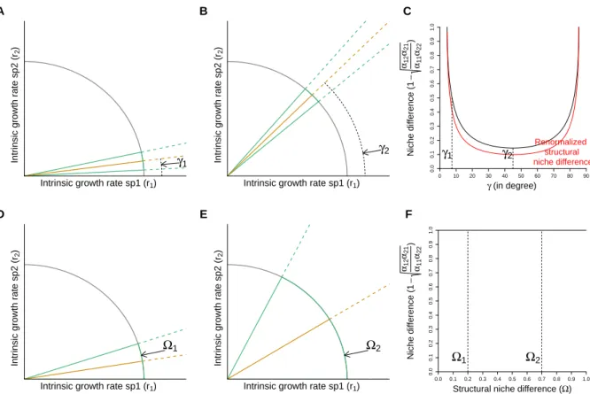
Figure S1 shows two extreme cases illustrating the subtle but fundamental difference between MCT’s and the structural frameworks. Specifically, the top panels (A-C) show that if the position of the feasibility domain (area formed by the inequalities) changes due to a changing competitive imbalance, a compensatory increase in the MCT niche

difference is required to yield the same structural analog of niche difference Ω. Similarly, the bottom panels (D-E) show that if one interspecific competition coefficient equals zero (i.e., one of the slopes lies on the border) any niche difference less than 1 will allow coexistence under MCT. By contrast, the structural approach is a geometric approach that quantifies the set of intrinsic growth rates leading to coexistence independent of whether the competition among species is balanced (and gives different Ω in the two cases depicted in panels d and e). Note that only the structural approach has a probabilistic interpretation. Indeed the structural-based measure of niche difference Ω gives the probability of having a feasible system, i.e., it is the probability of sampling a set of growth rates in the feasibility domain (assuming that the growth rates are sampled uniformly but with a fixed norm, where the direction of the vector of growth rates is sampled uniformly).

We may wonder if there is a way to incorporate the competitive imbalance into the structural approach. To do this, we first need to understand from where this fundamental difference is arising. MCT’s niche difference is deduced from the two inequalities (2), which give the condition of coexistence (assuming the stability condition satisfied). The two inequalities (2) are then combined into Equation (3), which describes the upper and lower bound that the ratio in intrinsic growth rates can tolerate to ensure coexistence. Then the competitive imbalance term is incorporated by multiplying each term of Equation (3) by the factor qα22α21

α11α12. This leads to the classical definition of niche

(13)

γ1 Intrinsic growth rate sp1 (r1)

Intrinsic growth rate sp2 (

r2

)

A

γ2 Intrinsic growth rate sp1 (r1)

r2 ) B 0.0 0.1 0.2 0.3 0.4 0.5 0.6 0.7 0.8 0.9 1.0 0 10 20 30 40 50 60 70 80 90 Niche dif ference ( 1 − α12 α21 α11 α22 ) γ (in degree) C γ1 γ2 Renormalized structural niche difference Ω1 Intrinsic growth rate sp1 (r1)

r2

)

D

Ω2 Intrinsic growth rate sp1 (r1)

r2 ) E 0.0 0.1 0.2 0.3 0.4 0.5 0.6 0.7 0.8 0.9 1.0 0.0 0.1 0.2 0.3 0.4 0.5 0.6 0.7 0.8 0.9 1.0 Niche dif ference ( 1 − α12 α21 α11 α22 )

Structural niche difference (Ω)

F

Ω1 Ω2

Figure S1: Differences between the MCT and the structural approaches. Panels A and B show the same area (Ω) between the two inequalities (green lines) but in different positions characterized by the angle γ between the border (x-axis) and the centroid of the area (orange line). Panel C shows the value of the classic niche difference as a function of γ. Note that in the structural approach, the structural analog of niche difference (Ω) does not change as a function of γ. The dashed lines correspond to the values of γ shown in Panels A and B. The red line in Panel C corresponds to the renormalized structural analog of niche difference. Panels D and E show different areas (Ω), where the bottom slope lies on the border (x-axis). Panel F shows the value of these areas calculated as the niche difference under the structural approach (x-axis) and the classic niche difference (y-axis). Note that the classic niche difference is always 1. The dashed lines correspond to the values of Ω shown in Panels D and E.

As explained in the main text, simple inequalities equivalent to the MCT’s ones for n-species do not exist. Therefore, there is no straightforward way to incorporate the competitive imbalance in the structural approach. Note that in the two species case, incorporating the competitive imbalance is equivalent to renormalizing the intrinsic growth rates of the two species by r1 → r1/

√

α11α12 and by r2 → r2/

√

α21α22. Then we

also need to renormalize the interaction strengths as follows " α11 α12 α21 α22 # −→ " α11/ √ α11α12 α12/ √ α11α12 α21/ √ α21α22 α22/ √ α21α22 # .

Finally, we can recompute the solid angle with the renormalized interaction strengths. For two species, the renormalized solid angle behaves in a similar way as the classical

(14)

niche difference (shown by the red line on Figure S1.C). More generally, in dimension n, we may renormalize the interaction strengths as follows

αij −→

αij n

pQn k=1αik

and compute the solid angle (Ω) based on the renormalized interaction strength. However, this renormalization as in MCT’s approach is informative if no interspecific interaction is close to zero (see discussion above). Moreover, the comparison of niche differences (at any n-dimensional side in the simplex, is only possible under a structural approach. Under MCT’s framework, as we would require to re-scale the matrix of competition coefficients for each pairwise case (or n-dimensional side in the simplex), each niche difference would lead to different units (defined by the particular re-scaling), making impossible their straight comparison across matrices or dimensions. In fact, to make all niche differences with the same units, one would need to remove the re-scaling, going back to the structural approach.

(15)

Appendix S6: Mathematical derivation and numerical

estimation of the structural analog of niche difference

Ω

The structural analog of niche difference is mathematically defined as the normalized solid angle of the cone defining the feasibility domain. We recall that this cone is generated by the column-vectors of the interaction strength matrix:

DF(α) = {r = N1∗v1+ N2∗v2+ · · · + Nn∗vn, with N1∗ > 0, N ∗ 2 > 0, . . . , N ∗ n > 0} , where α =    α11 · · · α1n .. . . .. ... αn1 · · · αnn   =     .. . ... ... v1 v2 . . . vn .. . ... ...     .

The solid angle of such a cone can be computed by the following multiple integration (for the mathematical derivation and details see Ribando, 2006):

Ω = 2 n_{| det(α)|} πn/2 Z · · · Z Rn≥0 e−xTαTαxdx.

The solid angle has been normalized such that Ω = 1 in absence of interspecific interaction (αij = 0, i 6= j). Moreover, by setting αTα = 1₂Σ−1, the above integration

transforms into: Ω = 2 n (2π)n/2p| det(Σ)| Z · · · Z Rn ≥0 e−xT 12Σ −1_x dx,

which is (up to a multiplicative factor of 2n_{) the cumulative distribution of a multivariate}

normal distribution centered in zero and of variance-covariance Σ. The cumulative distribution of a multivariate normal distribution can efficiently be estimated using the quasi Monte-Carlo algorithm developed by A. Genz (Genz and Bretz, 2009; Genz et al., 2016).

References

Genz, A., and F. Bretz. 2009. Computation of Multivariate Normal and t Probabilities. Lecture Notes in Statistics, Vol. 195. Springer-Verlage, Heidelberg.

Genz, A., F. Bretz, T. Miwa, X. Mi, F. Leisch, F. Scheipl, and T. Hothorn, 2016. mvtnorm: Multivariate Normal and t Distributions. R package version 1.0-5. R

(16)

Foundation for Statistical Computing. URL http://CRAN.R-project.org/package=mvtnorm.

Ribando, M. J. 2006. Measuring Solid Angles Beyond Dimension Three. Discrete & Computational Geometry 36:479–487.

(17)

Appendix S7: Geometric shapes of the feasibility

domain

Here, we explore the different geometric shapes of the feasibility domain and their effect on multispecies coexistence. To do this, we randomly generated 20 thousand globally stable communities with different number of species, where the interaction matrices were drawn following a niche framework (see below). For each generated community, its structural analog of niche difference Ω was calculated, and then different vectors of intrinsic growth rates r were sampled and used to compute the number of coexisting species and the structural analog of fitness difference θ. The number of coexisting species was computed by solving the abundances at equilibrium N_i∗ (abundances greater than zero are considered as coexisting species). The structural analog of fitness difference was computed by comparing the sampled vector r and the corresponding centroid of the feasibility domain rc.

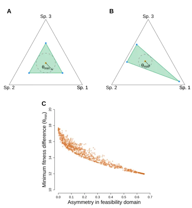
We find that for communities with more than 2 species, there is no longer the clear division between regions of coexistence and exclusion, as in the 2-species case (Fig. S1). While the combination of high structural analog of niche differences and low structural analog of fitness differences yield higher chances of coexistence as in the 2-species case, now communities with the same combination of structural analog of niche and fitness differences can have a different number of coexisting species. These findings reveal that, in contrast to the 2-species case, multispecies coexistence cannot be predicted with niche and fitness differences only. The reason is that two multispecies communities with the same structural analog of niche difference may not tolerate the same structural analog of fitness difference. This happens because various geometric shapes of the feasibility domain (defined by the pairwise interactions) can produce the same structural analog of niche difference Ω (Figs. S2A and S2B). This variable geometry implies that a community can tolerate a greater structural analog of fitness difference in some directions than others. The above limitations reveal a challenge when defining the structural analog of niche difference in systems with more than two competitors, and this involves taking into account the shape of the feasibility domain. Unfortunately this is not an easy task, but one possible solution involves computing the asymmetry of the feasibility domain. This asymmetry can be estimated by the variation among all the n-faces of the given

multidimensional cone. This can be computed by the variance of all the n-structural analog of niche differences generated by removing each of the n-species in the community independently. For instance, if we have a 3-species system, the feasibility domain will form a 3-dimensional cone and can be projected on the 2-dimensional simplex. The projection corresponds to a triangle, and each of its sides corresponds to the length of the feasibility domain of each pairwise interaction. If the pairwise interactions are symmetric and equal, this variance would be zero. The higher the variance is, the higher the

(18)

asymmetry of the feasibility domain.

Figure S2C shows that for distinct 3-species communities with the same structural analog of niche difference, the higher the variance or asymmetry in their feasibility domain, the lower their minimum structural analog of fitness difference that can be tolerated in any particular direction. Note that while the minimum structural analog of fitness difference is a good indicator of the level of tolerance under random perturbations, the natural variation in intrinsic growth rates may tend to fall in one particular direction. Thus, systems with high asymmetry do not need to be vulnerable systems necessarily.

Niche framework

We generated 10 thousand random matrices following a niche overlap framework (MacArthur and Levins, 1967; Levins, 1968). These matrices are by definition globally stable, requiring only to have feasible equilibrium points to fulfill our conditions of species coexistence. Specifically, these matrices were generated using the following procedure. For a matrix of dimension S, assuming a one dimensional niche space, the diet of species i is described by the niche utilization function. These functions are usually taken as a Gaussian-like curve:

gi(x) = ai √ 2πσi e− x−µi 2σ2 i ,

where σi is the niche width of species i, ai is the amplitude, and µi the diet center. Then

the competition coefficients are calculated as

αij =

Z

gi(x)gj(x)dx.

Therefore, we can write

αij = aiaj q σ2 i + σj2 e −1 2 (µi−µj )2 (σ2_i+σ2_j) .

Note that the matrix α is in general not symmetric, unless we assume the same niche width and niche amplitude for all species. Recall that these interaction matrices are by definition positive definite thus Volterra-dissipative, and therefore, a feasible equilibrium point is globally stable (MacArthur and Levins, 1967; Svirezhev and Logofet, 1983; Logofet, 1993).

(19)

A

verage number of coexisting species

3 2 1 0.0 0.1 0.2 0.3 0.4 0.5 0.6 0.7 0.8 0.9 1.0 0 10 20 30 40 50 60 70 80 90

Structural fitness dif

ference (

θ

)

A

verage number of coexisting species

10 9 8 7 6 5 4 3 2 1 0.0 0.1 0.2 0.3 0.4 0.5 0.6 0.7 0.8 0.9 1.0 0 10 20 30 40 50 60 70 80 90

Structural fitness dif

ference (

θ

)

B

Figure S1: Structural analog of niche and fitness differences for n-species com-munities. Panel A and B show, respectively, the average number of coexisting species in (globally stable) randomly generated communities of 3 and 10 species as a function of structural analog of niche (Ω) and fitness differences (θ). The darker (greener) the region, the more the expected number of species that can coexist with a given combination of structural analog of niche and fitness differences. Higher structural analog of fitness dif-ferences can be computed in combination with lower structural analog of niche difdif-ferences because of geometric constraints, and must not be interpreted as if lower structural analog of niche differences can tolerate higher structural analog of fitness differences.

(20)

Sp. 1 Sp. 2 Sp. 3 Sp. 1 θmin

A

Sp. 1 Sp. 2 Sp. 3 Sp. 1 θmin

B

0.0 0.1 0.2 0.3 0.4 0.5 0.6 0.7 10 12 14 16 18 20

Asymmetry in feasibility domain

Minimum fitness dif

ference (

θmin

)

C

Figure S2: Structural analog of niche, fitness, and asymmetry. Panels A and B show the projected feasibility domain of two distinct communities with 3 species. Both communities have the same structural analog of niche difference (green area of feasibility domain), but different geometric shapes (defined by their pairwise interactions). The black vectors inside the feasibility domains correspond to the minimum structural analog of fitness difference (θ) that can be tolerated in any direction. Panel C shows the minimum tolerated structural analog of fitness difference as a function of the asymmetry in feasibility domain. Each point corresponds to a different 3-species community, all with the same structural analog of niche difference (Ω).

(21)

References

Levins, R. 1968. Evolution in Changing Environments: Some Theoretical Explorations. Princeton University Press, USA.

MacArthur, R., and R. Levins. 1967. The Limiting Similarity, Convergence, and Divergence of Coexisting Species. Am Nat 101:377–385.