A continuum theory with long-range forces for solids

A Continuum Theory with

Long-Range Forces for Solids

by

Markus Zimmermann

Submitted to the Department of Mechanical Engineering

in partial fulfillment of the requirements for the degree of

Doctor of Philosophy in Mechanical Engineering

at the

MASSACHUSETTS INSTITUTE OF TECHNOLOGY

February 2005

@

Massachusetts Institute of Technology 2005. All rights reserved.

Author ...

Department of Mechanical Engineering

January 28, 2005

Certified by...

.

Rohan Abeyaratne

Professor and Department Head

Thesis Supervisor

A

Accepted by

MASSACHUSETTS INS1TTUTE OF TECHNOLOGY

MAY

[

5

2005

I

Lalt

nn

Lallit Anand

Professor and Graduate Officer

A Continuum Theory with

Long-Range Forces for Solids

by

Markus Zimmermann

Submitted to the Department of Mechanical Engineering on January 28, 2005, in partial fulfillment of the

requirements for the degree of

Doctor of Philosophy in Mechanical Engineering

Abstract

A non-local integral-type continuum theory, introduced by Silling [61] as peridynamic theory, is analyzed. The theory differs from classical (local) continuum theories in that it involves long-range forces that act between continuum particles. In contrast to existing non-local theories, surface tractions are excluded. As consequence, the theory is applicable off and on defects and interfaces: cracks and phase boundaries are a natural part of the body, and do not require special treatment. Furthermore, as the model loses "local stiffness", the resistance to the formation of discontinuities is reduced.

The theory can be viewed in two ways: It is a multi-scale model in that it can be applied simultaneously on the atomistic level and on the macroscopic level with a smooth interface between the two regimes. Alternatively, it can be used as a purely phenomenological macroscopic model that still works off and on defects. Forces of microscopic range may represent the interaction of an underlying microstructure such as discrete particles. Forces of macroscopic range are not necessarily physical and are justified by their effective behavior.

A meshless numerical approximation technique is implemented for the macroscopic model and used to simulate brittle fracture. If the internal length of the simulated peridynamic body is small compared to its macroscopic dimensions, then the simula-tion results agree well with linear elastic fracture mechanics. In contrast to classical fracture mechanics, however, the crack path does not need to be known in advance. Thesis Supervisor: Rohan Abeyaratne

Acknowledgements

I would like to express my deep gratitude to Professor Rohan Abeyaratne for his guidance through my years at MIT. I am grateful for our discussions, his helpful advice and his support.

I also would like to give thanks to the members of my thesis committee, Professor Nicolas Hadjiconstantinou and Professor David Parks, for important ideas and critical discussions.

I am grateful to Sandia National Laboratories for supporting my research. I thank Doctor Stewart Silling for discussions and helpful comments.

I am indebted to Professor Yves Leroy who hosted my stay at the Ecole Polytech-nique. The stay was made possible by the Embassy of France and the Chateaubriand Fellowship. I thank Professor Lev Truskinvosky for our discussions and the insights he gave me.

I would like to thank Michael Demkowicz and Vadim Roytershteyn for numerous inspiring discussions during my time at MIT. Many thanks to Michael Demkowicz and Olaf Weckner for reviewing the thesis and their helpful comments.

Contents

1 Introduction 1.1 Problem Statement . . . . 1.2 Existing Approaches . . . . 1.3 Scope . . . . 2 Fundamentals

2.1 Mass and Motion . . . . 2.2 Forces . . . . 2.2.1 Balance Laws . . . . 2.2.2 Interaction Forces and Links . . . 2.2.3 Equation of Motion . . . . 2.3 Balance of Mechanical Power and Energy 2.4 Constitutive Theory . . . . 2.4.1 Objective Constitutive Relations 2.4.2 Homogeneity and Isotropy . . . .

2.4.3 Elasticity . . . . 2.4.4 Inelasticity . . . .

2.5 Initial Boundary Value Problems . . . .

2.5.1 Local Formulation with Equation of Motion . . . 2.5.2 Variational Formulation . . . . 2.5.3 Reaction to Surface Displacements and Tractions 2.6 Equilibria . . . .

2.6.1 Equilibrium Problem and Equilibrium Condition.

17 17 18 21 23 23 25 25 27 28 28 32 32 33 35 37 40 40 40 42 43 43

2.6.2 Variational Equilibrium Problem . . . . 2.6.3 2.7 Stress 2.7.1 2.7.2 2.7.3 2.7.4 2.8 Linear 2.8.1 2.8.2 2.8.3 2.8.4 2.8.5 2.8.6 2.8.7

Stationary and Minimum Potential Energy . . . . . . . . Non-local Stress . . . .

Stress as Energy-Conjugate Quantity . . . . Cauchy's Dynamic Notion of Stress . . . . Non-local Stiffness . . . . Theory . . . . Linearization . . . . Dispersion Relation . . . . Waves at the Undeformed State . . . . Infinitesimal and Small Scale Stability . . . . Existence and Uniqueness of Equilibrium Solutions Plane Deformation . . . . One-dimensional Plane Deformation . . . .

3 Comparison of Theories

3.1 Introduction . . . . 3.2 Formal Agreements with Other Models . . . . 3.2.1 Non-linear Strain Gradient Models . . . . 3.2.2 Non-linear Classical Elasticity . . . .. 3.2.3 Linear Integral-type Models with Strain Field 3.2.4 Atomistics . . . . 3.2.5 Consequences for Structure-less Materials

3.3 Linear Elastic Behavior of Different Models . . . .

3.3.1 Role of Dispersion Relations . . . . 3.3.2 Discrete System . . . . 3.3.3 Classical Local Elasticity . . . . 3.3.4 Strain Gradient Model . . . .

3.3.5 Integral-type Model with Strain Field . . . .

43 44 44 45 47 49 50 50 53 54 55 57 57 59 61 61 62 62 64 66 67 69 70 70 72 73 73 75 . . . . 43

Peridynamic Continuum . . . . Dispersion Relations and Local Stiffness . . . . Role of Brillouin Zone . . . . 4 Force Laws

4.1 Linear Atomistic-peridynamic Force Law . . . 4.2 General Atomistic-peridynamic Force Law . . 4.3 Force Law for Heterogeneous Materials . . . . 4.4 Force Law with Resolution Length . . . . 4.5 Definition of the Elastic Internal Length . . . 4.6 Interpretations of Internal Lengths . . . . 4.7 Interpretation of Displacement Discontinuities 4.8 Application of Boundary Conditions . . . . 4.9 Interpretation of a Peridynamic Continuum 5 Solution Techniques

5.1 Introduction . . . . 5.2 Perturbation-type Analysis . . . . 5.2.1 Problem . . . . 5.2.2 Approximation Method . . . . 5.2.3 Example I: Discontinuity at Interface . 5.2.4 Example II: Two Interfaces . . . . 5.2.5 Summary . . . . 5.3 Numerical Methods . . . .

5.3.1 Cutoff in the Reference Configuration 5.3.2 Collocation Method . . . . 5.3.3 Ritz and FE Method . . . . 5.3.4 Time Integration . . . . 79 79 81 84 87 89 90 91 92 92 95 95 96 . . . . 96 . . . . 98 . . . . 106 . . . . 108 . . . . 110 . . . . 110 . . . . 110 . . . 111 . . . . 113 . . . . 115 6 Brittle Fracture 6.1 Basic Concepts . . . . 117 117 3.3.6 3.3.7 3.3.8 75 76 77

6.1.1 Particle Separation . . . . 6.1.2 Strength . . . . 6.1.3 Surface Energy . . . . 6.1.4 Cracks . . . . 6.2 Example . . . . 6.3 Griffith Criterion . . . . 6.4 Incipient Crack Growth in a Strip . . . . 6.4.1 Introduction . . . . 6.4.2 Infinite Strip in Local Theory . . . . 6.4.3 Perturbation Analysis of Infinite Strip 6.4.4 Numerical Simulation of Finite Strip 6.4.5 Summary . . . . 6.5 Autonomous Growth of a Curved Crack 7 Conclusions

A Derivations

A.1 Global and Local Balance of Momentum A.2 Action Equals Reaction . . . . A.3 Pair-wise Forces are Central Forces . . . . . A.4 Global Power Balance . . . . A.5 Internal Work Rate . . . . A.6 First Time Derivative of Elastic Energy . . A.7 Stationarity of Potential Energy . . . . A.8 W aves . . . . A.9 Infinitesimal Stability . . . . A.10 Small Scale Stability . . . .

A.11 Transition to Strain Gradient Model . . . .

A.12 Transition to Classical Elasticity . . . . A. 13 Transition to Integral Model with Strain . . A.14 Energies in Perturbation Analysis . . . . .

117 118 118 119 120 124 126 126 127 128 130 139 139 143 147 147 . . . . 148 . . . . 150 . . . . 15 1 . . . . 152 . . . . 152 . . . . 155 . . . . 156 . . . . 158 . . . . 159 . . . . 160 . . . . 162 . . . . 16 2 . . . . 165

B Definitions

C Stiffness Distributions 169

List of symbols

1 b bint b, C C C= FTF C C Ltt 7= £ E E ej er = r/r ec = V/( F =2 f

unity tensor of second order external body force

body force due to particle interaction on Q total force

prescribed external force on b

classical stiffness tensor of fourth order non-local stiffness tensor of second order right Cauchy-Green tensor

stiffness distribution; in section 5.2 only: C = C

normalized stiffness distribution linear strain tensor

strain in id 1 link strain

change of distance in id Lagrangian strain

total kinetic energy Young's modulus

unit vector in coordinate direction unit vector pointing from y to y' unit vector pointing from x to x' deformation gradient

2y, surface energy

h characteristic distance of discretization points

ho horizon (i.e. radius of support) of

f

in the reference configuration

he cutoff radius

Isym symmetric identity tensor of fourth order

k wave vector

k wave number

A Lam6 constant

A normalized internal length in section 5.2

Am macroscopic stretch

A,, = r/ link stretch

1 internal length

A Lame constant, shear modulus

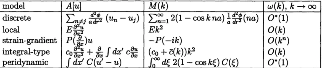
Mi stiffness moment of order j

M(k) one-dimensional non-local acoustic tensor

M non-local acoustic tensor (second order)

v Poisson's ratio

Nj dimension-less stiffness moment of orderj Q body, set of positions in reference configuration OQ boundary of a body

QU part of body on which displacements (or positions) are prescribed OQU boundary of Qu

Qb part of body that is subject to external body forces (which may be zero)

O0b boundary of Qb

QY deformed body; set of positions in current configuration

w wave frequency

T total Helmholtz free energy Helmholtz free energy density -pair-wise Helmholtz free energy Tei total elastic energy

?Pel OIel P PO

r=IrI

?Ie r/Jy -0 O 0 2pk .4 = n U =V - X U =y - X Wdi,, (Wdis,) IWdiss (Wdi,,) Wdiss (?bd 8s) Wext Wext Wint Wint wbint S= X' - 2 X

x

y y X

elastic energy density pair-wise elastic energy mass per current volume mass per reference volume

distance vector in current configuration

2d/3d: scalar distance in current configuration (always positive) 1d: distance with sign indicating the direction

Cauchy stress tensor first Piola-Kirchhoff stress second Piola-Kirchhoff stress

normal velocity of a surface in the reference configuration displacement vector

displacement in id

prescribed displacement on Q. (rate of) dissipated energy

(rate of) dissipated energy density (rate of) pair-wise dissipated energy rate of total external work

potential of total external work rate of internal work

rate of internal work density rate of pair-wise internal work

distance vector in reference configuration

scalar distance in reference configuration (always positive)

position in reference configuration and identification label of a particle position in reference configuration in ld

position in current configuration position in current configuration in id vector of generic internal variables

Notation: Constitutive functions have a hat. Integral transforms are marked with a bar.

Chapter 1

Introduction

1.1

Problem Statement

Solid bodies usually have an intractable number of degrees of freedom and only few of them are relevant for their macroscopic behavior. Classical continuum mechanics is a powerful tool, because it eliminates the detailed microstructure while keeping what is macroscopically relevant, creating mathematical models that can be treated either analytically or numerically. Material behavior is expressed by relations between stress and strain, which are the response of a representative volume element of the material to homogeneous deformation. The size of the volume element depends on the resolu-tion of the model. It can be on the order of Angstroms for crystal lattices, microns for metals with grains, or centimeters for heterogeneous materials like concrete.

Classical continuum models are applicable when the characteristic length of the deformation is sufficiently larger than the representative volume element of the body. If deformations localize, the continuum model begins to break down, and finally fails when deformations are non-smooth or discontinuous. The inability to describe local-ized deformation is reflected in the mathematical structure of continuum mechanics. Constitutive relations are formulated with deformation gradients (and their deriva-tives). If a deformation is non-smooth, the deformation gradient is not defined in a classical sense. This is the case for cracks where displacements are discontinuous across the crack faces or for phase boundaries where the strain field is discontinuous.

The classical remedy has been to treat regions that have an undefined deformation gradient separately. Crack lips are considered body surfaces with particular boundary conditions. Crack tips satisfy a particular energy balance that is different from the rest of the body. Phase boundaries are surfaces inside the body that satisfy particular jump conditions and kinetic relations.

This treatment relies on efficient bookkeeping of degrees of freedom. The bulk part of the body is sufficiently described by regular continuum mechanics, while the effective behavior of the defects is described by physical laws containing only the in-formation that is relevant for the macroscopic behavior of the body. It may be difficult and costly, however, to keep track of defects. Analytical work becomes more com-plicated with more boundaries and irregular geometries. Numerical approximation methods must rely on expensive techniques like remeshing to make the propagation of defects possible. In addition, the physical laws governing defects may not be suffi-ciently characterized. This is why a theory that works off and on defects is useful.

The peridynamic theory introduced by Silling [61] is a continuum theory that does not require well-defined deformation gradients. Constitutive information is provided entirely on the basis of positions of (continuum) particles of the body. It resembles the formal structure of molecular dynamics in that it sums forces between pairs of particles. Therefore, it provides a good framework for including relevant parts of the microstructure into the constitutive description of the body. As particles interact at finite distance, the theory is non-local and has an internal length.

The purpose of this thesis is to explore the ability of peridynamic theory to model defects as a natural part of the body without special treatment.

1.2

Existing Approaches

Non-local Theories. Material models that are invariant with respect to rescaling of spatial variables are called simple by Noll [54], strictly local by Rogula [58] or just local by Kunin [48]. These materials have no internal characteristic length with

Models that are not invariant with respect to rescaling of spatial coordinates are called non-local and have an internal length. This makes them better suited for mod-eling phenomena at small scales. Weakly non-local models have constitutive relations that depend on higher order gradients. For a general treatment of gradient models see Rogula [58], for a variational formulation, see Mindlin [53]. For strain gradient plas-ticity see Fleck and Hutchinson [31]. In Strictly non-local or integral-type non-local models, the stress depends on the deformation of a finite environment of a contin-uum point. Early studies of Non-local Elasticity aimed at improving the agreement between continuum theories and crystal lattices (see Rogula [59]). Attention was typically focused on removing stress and strain singularities at the cores of disloca-tions (see Eringen [28]) or crack tips (see Eringen [29]), determining elastic energies of defects (see Gairola [35]), or accounting for boundary layers in the deformation of small bodies (see Picu [55]). Overviews of the theory can be found in Kr6ner [46], Rogula [59], and Kunin [48, 49]. For a recent review focused on lattice dynamics and phonon dispersion, see Chen et al. [19]. In all these cases, the non-locality of the model represents the non-local character of interatomic forces.

A different motivation for non-local models comes from statistical continuum me-chanics. Here, long-range forces describe the effective behavior of heterogeneous ma-terials. Their interaction length is associated with the statistical correlation length of heterogeneities, see for example Kr6ner [47] and Kunin [49]. For recent work in the context of elastic deformation of composite materials, see Drugan and Willis [24]. A mixed probabilistic-atomistic approach is presented in Banach [8].

Extensions of integral-type non-local theories to plasticity were proposed by Erin-gen [27] and to damage mechanics by Bazant [10]. Non-local mechanics found ample application in the modeling of the failure of brittle heterogeneous materials such as concrete. Concrete undergoes strain softening under failure, making the well-posedness of a mathematical description depend on the existence of an internal length in the model (see Bazant [11] or Jira'sek [43]). The internal length was again a sta-tistical length accounting for the heterogeneity of the material. For a recent survey of non-local integral-type theories applied to plasticity and damage of heterogeneous

materials, see Bazant and Jirisek [12].

For current work on non-linear integral-type non-local models in the context of phase transitions see Truskinovsky and Zanzotto [70] and Ren and Truskinovsky [57]. Most non-local models improve the ability to model the microstructure of a ma-terial and its defects. They share the property, however, that they (with a few exceptions) rely on spatial derivatives of the displacement fields in their constitutive description.

Handshake Methods. A different approach that models the effect of defects splits the body into different regions. Each region is simulated by a model on the appro-priate scale. This is an efficient way to account for the microstructure and to save resources at the same time. Typically, a macroscopic Finite Element model is coupled with Molecular Dynamics, e.g., in the quasicontinuum method which was introduced by Tadmor et al. [66] and recently reviewed by Miller and Tadmor [52]. Sometimes, even the quantum scale is included, see Abraham et. al. [5] or Broughton and Abra-ham [16]. The disadvantage of handshake methods are wave reflection or unphysical "ghost forces" at the interfaces of different scales. In addition, interfaces require special attention. They need to be moved, which typically necessitates remeshing.

Macroscopic Treatment of Defects. Cohesive surface models like the one used by Camacho and Ortiz [17], can create cracks in arbitrary directions by letting Finite Elements separate. The advantage of this approach is that macroscopically relevant properties (like friction on crack faces) can be represented efficiently. However, it is necessary to follow every crack tip individually.

The Virtual Internal Bond Model proposed by Gao and Klein [36] provides a macroscopic approach derived directly from atomistic laws. A Finite Element frame-work represents an atomistic structure accurately for small element sizes. Again, fine spatial resolution of the numerical framework is necessary at the zones of interest. Remeshing is therefore necessary.

Work on peridynamic theory. The theory was first introduced by Silling [61] and applied to the numerical simulation of impact in [62]. Silling and Bobaru [63] developed a peridynamic constitutive model for rubber and applied it in the numerical simulation of failure in membranes and fibers. Initial analytical work on the theory was done by Silling et al. [64] and Weckner and Abeyaratne [72].

1.3

Scope

Chapter 2 provides a systematic presentation of the fundamentals of peridynamic the-ory. The local equation of motion postulated by Silling [61] is helpful in immediately understanding the formal similarity of the theory to atomistic systems and providing an important initial motivation for the theory. The approach adopted here is different in that it starts from global balance laws and then derives the local laws, as in classical continuum mechanics. The chapter puts special emphasis on discontinuous and non-smooth deformations. It is shown that the balance of linear and angular momentum, the balance of mechanical power and energy, and the variational formulation do not have a jump term which would require special treatment of discontinuity surfaces. A basic constitutive theory is presented for plastic materials and materials that can undergo failure. A notion of stress is introduced and motivated. The framework of linear peridynamic theory is presented and applied to wave dispersion. It is shown how a body can become unstable due to the action of long-range forces. The special equations of motion for plane and one-dimensional deformations are derived.

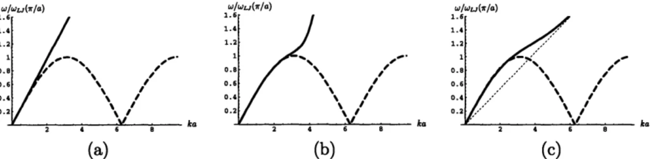
Chapter 3 explores how peridynamic theory relates to other models of solid bodies. In particular, it is shown how peridynamic theory can be approximated by a strain gradient theory of infinite order (if the deformation is sufficiently smooth), how local continuum theory is recovered by letting the internal length disappear, and finally, how atomistic theory is included in the peridynamic theory as a heterogenous body with its mass concentrated on discrete points. All the continuum theories are then contrasted with focus on their ability to approximate the linear elastic behavior of a discrete system. The role of the Brillouin zone is discussed.

Chapter 4 presents several force laws to either approximate atomistic dynamics or to be used on a macroscale. Of particular importance for general macroscopic bodies are force laws with resolution length. The internal length and the peridynamic continuum are interpreted.

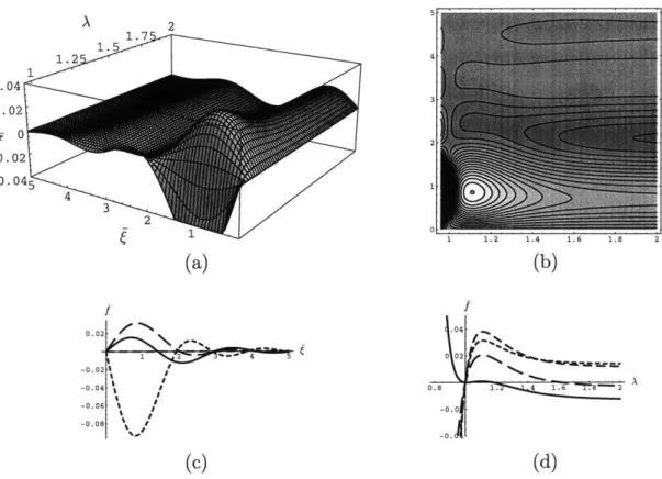
Chapter 5 provides a brief review of analytical solution techniques. A perturbation method is introduced that captures the behavior of displacement discontinuities. The Ritz approximation method and the collocation method are presented.

Chapter 6 defines the basic concepts of brittle material failure in peridynamic theory. Crack propagation in a strip is simulated to verify the ability of peridy-namic theory to predict the onset of failure. Finally, autonomous crack growth in an asymmetrically pre-cracked body is simulated.

For clarity, most derivations of fundamental relations were moved to the appendix. The reader is encouraged to refer to them as necessary.

Chapter 2

Fundamentals

2.1

Mass and Motion

A body is modeled in peridynamic theory as a continuum. It consists of a continuous set of material points or particles and is denoted by 1. Particles are identified by their position x in the reference configuration. They are particles in the continuum sense (see Truesdell and Noll [691) and are assigned a mass density, rather than a mass. The mass density at x represents mass per reference volume. It does not depend on time and is denoted by the bounded and piece-wise continuous function po = pO(x).

The position y of a particle x at time t is given by the motion y = y(x, t). Displacements from the reference configuration into the current configuration are denoted by u = y - x. A continuum particle has only three translational degrees of freedom and is therefore a medium of simple structure in the sense of Kunin [48]. The material time derivatives of y are the velocity i = y(x, t) and the acceleration

y = 9(X, t).

If a particle is separated from the neighborhood it had in the reference configura-tion, the fields of displacements and positions are discontinuous. It is assumed that y is bounded and at least piece-wise continuous, meaning that at least some parts of the body will stick together rather than losing connection entirely. The magnitude of

a discontinuity is quantified by the jump operator

[[p]] = [[p]](x, n, t) = lim [p(x + en, t) - p(x - en, t)]. (2.1)

A discontinuity surface S = S,(t) in the body Q is defined as the set of points x on which the jump operator applied to the quantity of interest, here p, gives a non-zero value. Note that this surface lies in the reference configuration. Assume that all surfaces are piece-wise smooth, but not necessarily connected. The vector n will from now on be used in this context as normal vector of the surface S, at x. On smooth parts of the surface, the normal surface velocity reads 4 = An, with A being

the propagation speed. On the boundaries of smooth parts, like kinks or lines where the surface ends, the surface may propagate into the non-normal direction.

A crack in the classical sense' is represented by a discontinuity surface S, associ-ated with the field of positions where

[[y]] -n > 0. (2.2)

The boundary line of this surface inside the body 1 represents a crack front.

A phase boundary in the classical sense is represented by a surface SF, associ-ated with a discontinuous field of deformation gradients. Following Abeyaratne and Knowles [3, page 348], the continuity of y at all times implies that at each instant of time A[[y]],esp = 0 and therefore

[[]] = -[[F]]An. (2.3)

1_{a definition of a crack in a non-classical sense that is more meaningful in the context of this} theory is given in chapter 6

2.2

Forces

2.2.1

Balance Laws

The sum of all forces acting on a continuum particle of the body is represented by the density field bt0r with the dimension of force per reference volume. Surface tractions

are excluded from the model. Sometimes bt,, is also referred to as "force", in particular when the theory is compared to atomistic theories. A force is then to be understood in a generalized sense, including classical forces and force densities.

bt,, is assumed to be bounded: singular or point forces are excluded, unless oth-erwise stated. The effects of concentrating forces in a limit process are discussed in section 2.5.3. Forces can be due to the deformation of the body or external sources, e.g., gravity. A body S has to satisfy the global balance of linear momentum

dIjpo dV= bt, dV (2.4)

and the global balance of angular momentum

d y x poi dV = y x bt0s dV. (2.5)

Any part of a body Q is a also a body, which by itself has to satisfy both global balance laws. A consequence of this is that (2.4) and (2.5) are equivalent to two local balance laws, the local balance of linear momentum

po = btot, (2.6)

and the local balance of angular momentum

y x (poy - btot) = 0, (2.7)

respectively. The equivalence is shown in the appendix A.1. Both local balance laws (2.6) and (2.7) have to be satisfied almost everywhere on 0.

The equivalence of global and local balance laws holds without extra jump con-ditions on discontinuity surfaces. There are concon-ditions on certain discontinuity sur-faces - but they are implied by both, the local and the global balance of linear momentum.

An important example is the condition on the discontinuity surface SP0? associated with the specific linear momentum poY. Such surfaces occur when a discontinuity in the field of positions (like a crack in the classical sense) opens up or when a discontinuity in the field of deformation gradients moves (like a shock or a classical phase boundary). In these cases, [[jj]] = 0. A consequence of the conservation of linear momentum is that the normal speed of So,,, has to be zero, as shown in the appendix A.1. This implies that, first, a discontinuity in the field of positions, e.g., a crack in the classical sense, can only extend through its crack front but cannot propagate in its normal direction. Second, shock waves in the classical sense do not exist. A phase boundary in the classical sense cannot move in its normal direction.

The local balance of linear momentum (2.6) implies the local balance of angular momentum (2.7). Due to the equivalence to their global forms, it can be stated in more general terms that conservation of linear momentum implies the conservation of angular momentum.

In summary, removing surface tractions from the continuum model has the fol-lowing consequences:

1. Stress tensors do not naturally appear as a field quantity.

2. Jump conditions are not complementary to local balance laws, but rather a consequence of them.

3. Surfaces of discontinuous deformation gradients Sp, like shock waves or phase boundaries, cannot propagate in their normal direction.

4. The balance of angular momentum is a consequence of the balance of linear momentum.

2.2.2

Interaction Forces and Links

Two kinds of forces act on a continuum particle: interaction forces bene that the body exerts on itself, and external forces b, the source of which lies outside the body. They sum up to

btot = bint + b. (2.8)

The interaction forces are required to be such that in the absence of external forces the body does not change its linear or angular momentum. Thus, from (2.4) and (2.5) follows that

J

bint dV = 0 (2.9)

and

/

V

x bint dV = 0, (2.10)

respectively. An arbitrary subsection of the body Q,2

b C f also constitutes a body,

and (2.9) and (2.10) have to be satisfied for Gsub as well.

A two-body type interaction is assumed2_{. One restriction of this assumption is}

that Poisson's ratio has to be v = 1/4, as shown in section 2.7.4. Ways to remove this restriction involve multi-particle interaction. More complicated interaction forces are not considered here to keep the formal structure of the theory simple.

A link of two continuum particles is defined as their ability to exert forces on each other. Alternatively, a link may be called bond. It should then be carefully distinguished from atomistic or chemical bonds.

The interaction force acting on x is the sum of all pair-wise forces

f

= f(x', x, t) exerted by particles x':

bint(x) = dV'

f(x',

x, t). (2.11)

Combining (2.11) with (2.9) and (2.10) yields, first, the microscopic version of actio 2

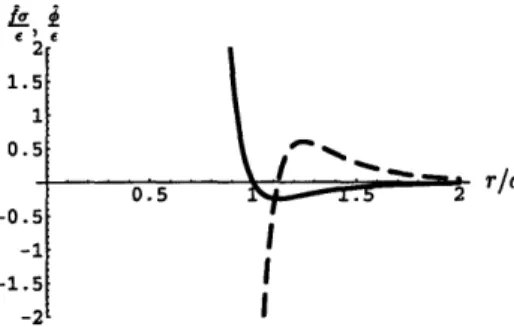
Two-body potentials are used in atomistic simulations to understand the qualitative behavior of bodies. A typical example is the Lennard-Jones 12-6 potential, see Allen and Tildesley [6, chap. 1.3]. For better agreements with real systems, multi-body potentials are preferred, e.g., the embedded atom potential for the simulation of metals, see Daw et al. [23].

= reactio (see derivation in the appendix A.2),

f(x', x, t) = -f(x, X', t), (2.12)

and, second, the requirement that

f

be a central force (see A.3),

f

li

er f = fe, (2.13)

where f = f(x', x, t).

2.2.3 Equation of Motion

The equation of motion is the local balance of linear momentum (2.6) combined with the assumption that external and interaction forces act on a continuum particle, and that interaction forces are pair-wise central forces:

po(x)(x, t) =

j

dV' f(x', x, t)er + b(x, t). (2.14) This is an integro-differential equation reminiscent of the equation of motion in molec-ular dynamics.

2.3

Balance of Mechanical Power and Energy

General Balance of Power and Definitions. The balance of energy can be de-rived from the local balance of momentum. Unlike in classical theories, no jump terms emerge on discontinuities of the displacement or the strain field. For the derivation, see appendix A.4. The general global power balance reads

dE + Wint = Wext, _(2.15)

where E is the kinetic energy

E = poi -i dV, (2.16)

and Wint is the rate of internal work

Tint = - bt -i dV, (2.17)

and Wext is the rate of external work

ext= b dV. (2.18)

The potential of external work is defined as

Wext = b - u dV. (2.19)

If the external force field does not change with time, then Wext = AWext.

A useful and intuitive expression for the rate of internal work is derived (in the

appendix A.5) from (2.11), (2.12) and (2.13) and the definition r = y' - y:

Tt = dV dV' ft. (2.20)

The rate of pair-wise internal work can then be identified as

int = wint(', X, t) = ft.

The rate of internal work density reads

Wint = Wint (x, t) = dv' zbj, (2.21)

where the integral adds the work done on a particular link to the work density at both points x' and x at equal share (therefore the factor of 1).

Helmholtz Free Energy. To keep the similarity to the formal structure of clas-sical continuum mechanics, constitutive information is contained in a potential that resembles the Helmholtz free energy when the temperature is fixed. The energy that is associated with the deformation of a pair of particles is called pair-wise Helmholtz free energy 0 = 0 (x', x, t). The Helmholtz-free energy is a general concept that

can be used for dissipative and non-dissipative processes, with or without internal variables (see section 2.4), or an explicit temperature field.

Similarly to (2.21), the Helmholtz free energy density is defined as

0 = (x, t) = dV' V(x', x, t). (2.22)

and the total Helmholtz free energy reads

XF = XI(t) = dV (x, t). (2.23)

Dissipation. In a purely mechanical setting, dissipated energy is defined as the part of internal work that is not stored as Helmholtz free energy, and, thus, not available to do mechanical work anymore. Dissipation is the rate of dissipated energy and is required to be zero or positive for each link. For the pair-wise dissipation the Clausius-Duhem-type inequality

d

?bdiss = bdiss (X1, X, t) = Tbint - -tO>0 (2.24)

has to be satisfied. The total dissipation, which is also required to be zero or positive, is defined as

WTis = Wdi,(t) = Wint - d ;> 0. (2.25)

dt

For general dissipative processes, the pair-wise Helmholtz free energy depends on internal variables, see section 2.4,

where

C

denotes a set of generic internal variables. The non-equilibrium force is defined by

fne= - . (2.26)

Non-equilibrium forces may be viscous forces, for example. From (2.24) follows that

diss = fneq +0 w

implying the restrictions on

fneq

fneqt > 0, and on

8>

0.

Non-dissipative Processes and Conservation of Energy. If the pair-wise Helmholtz free energy depends only on the current state of deformation, then it is called pair-wise elastic energy 'Oel (r, x', x). The elastic energy density is defined as

'l ei(X, t) = - dV' iPei(r, x', x )

2 and the total elastic energy as

'ei(t) = dV e(x ,t).

It is shown in the appendix A.6 that the time derivative of Tel does not include jump terms in the presence of discontinuities, provided that motions satisfy the balance of linear momentum. Therefore,

-ei= dV - dV' i], (2.27)

If a body has only elastic energy and the non-equilibrium forces are zero, pairs do not dissipate energy because of (2.24). Then, by (2.20) and (2.27),

int ~- 'Pet dt and finally with (2.25)

Wdis = 0,

without jump terms. By contrast, bodies in local theories may dissipate energy at moving strain discontinuities, see, e.g., Abeyaratne et al. [1]. In peridynamic theory however, the dissipation is zero if the force law is elastic.

If the external force field does not change with time, i.e., b = b(x), the integral of

the power balance (2.15) is the energy conservation law for non-dissipative processes,

E + 'Pei = West. (2.28)

2.4

Constitutive Theory

2.4.1

Objective Constitutive Relations

The magnitude of the pair-wise interaction force is determined by the deformation history of the particles x' and x, formally expressed by a constitutive relation

f = f(x', x, t) = f[y(x', t), y(x, t), x', x] (2.29)

where f[y', y, x', x]t is a functional that requires two time-dependent motions as arguments.

Constitutive relations are required to obey the rules of material objectivity. Let there be a motion of a material point that is seen by one observer as y = y(t), while a different observer sees y* = y*(t). Both observers have the same time. The frames of the two observers rotate by

Q

= Q(t) and translate by d = d(t) relatively to each

other. Then y and y* are related by

y* = Qy + d. (2.30)

If the two observers measure magnitude and orientation of the same force from their individual perspective, they may obtain different values. The first requirement of material objectivity is that the measurements differ by the rotation of their reference frames

Q,

i.e.,

f*

=

Qf;

from (2.13) follows that

f*

=

f.

As a second requirement, both forces have to be given by the same constitutive relation. Thus,

f

has to satisfy

[y*, y*, X', X]t = f[y' Y, X', X]t, or with (2.30)

f[Qy'

+ d, Qy + d, x', x]t =

f[y',

y, x', x~t

for arbitrary Q and d, i.e., for arbitrary changes of reference frames. Due to this arbitrariness, the pair-wise force can only depend on the scalar distance (history)

r = y' - _{y of the two particles, i.e.,}

f = f[r, x', X] . (2.31)

Any constitutive function derived from the relation (2.31) keeps this structure.

2.4.2 Homogeneity and Isotropy

A constitutive relation is homogeneous if it is invariant under a translation d of the reference configuration to any other point pertaining to the same homogeneous part. In other words

f[r, a', x]t = f[r, x'+ d, x + d]t. (2.32) for all admissible d. Then, on this homogeneous region

holds with t = x' - x.

A constitutive relation is isotropic at x, if the interaction forces between x and particles from its environment x' do not depend on their spatial orientation in the reference configuration. The orientation of two particles is contained in the distance vector t = x' - x, with which the constitutive relation (2.31) can be equivalently rewritten as

f

= f[r, t, x]t. (2.34)

Isotropy for x implies that

f[r, t, x]t = f[r,

Qt,

x]t (2.35)

for arbitrary rotations

Q.

Consequently, the most general isotropic constitutive rela-tion at x is

f = f[r, , x]t. (2.36)

In many practical problems, the body of interest has a constitutive relation that is homogeneous and isotropic, i.e.,

f

= f[r, ]t. (2.37)

Undergoing a permanent deformation with failure or deforming plastically may change the material behavior of a body, and thus its homogeneity or material symmetry. Close to a crack lip, e.g., the interaction with the part of the body beyond the crack was eliminated by the propagating crack. In the sense of the definitions above, this part may have homogeneous or isotropic constitutive relations, and still behave non-homogeneously or anisotropically. Due to the non-local character of the theory, isotropy and homogeneity at a point x may be affected by a deformation process beyond its immediate neighborhood.

2.4.3

Elasticity

General Elastic Force Function

If the pair-wise interaction force

f

depends only on the current deformation of a pair of particles rather than on its deformation history, the constitutive relation is called elastic. For a pair of particles x' and x the force is given by

f = f(r, X', x), (2.38)

or by the potential ?ei with

f = (r, x', x). (2.39)

The potential Oel is the pair-wise elastic energy, as defined in section 2.3. It is of the type of a Helmholtz free energy and is used under the assumption that, first, the temperature is constant and, second, V)e depends only on the current deformation. For different forms of the Helmholtz free energy that do not only depend on the current state of deformation, see section 2.4.4.

Separable Force Functions

A special intuitive simplification of the force function is obtained by assuming that the interaction force is the product of a modulus E(x', x) and a possibly non-linear constitutive function

s

depending on the strain of a link e, = r/ - 1

f(r, ', X) = E(x', x) s(es). (2.40)

In the isotropic case, when f(r, ) = E( )s§(en), s can be measured in an experiment: Let F = (enl + 1)1, then ao = 5A8(ei)1, where A is Lame's constant, see section 2.7. At a displacement discontinuity, the strain of a link is unbounded for -+ 0. Therefore, the functions E and s have to be chosen appropriately in order to ensure regular behavior.

Linear-Elastic Force Functions

Key ingredient of an elastic force function that is linear in the deformation is the stiffness distribution C(x', x) and the reference force fo(x', x), representing the force exerted by particle x' on x in the undeformed reference configuration:

f(r, x', x) = C(x', x)(r - ) + fo(x', X). (2.41)

More specifically, the force function for an isotropic and homogeneous material with zero-valued reference force reads

f(r,

)

= C()(r -

).

(2.42)

All constitutive information is now contained in the stiffness distribution C. (2.42) is also a separable force function with C()6 = E(x, x') and s(a) = a - 1.

Non-linear force functions

f

can be approximated by (2.41) or (2.42) by setting C(x',x) = (6, X',x), fo(x', x) = f(6, x', x) or C() = ( ) respectively.

The general vectorial force between particles

f

= fe, cannot be linear in r due to the kinematic non-linearity in er = r/r. Linearity of the scalar force function

J

is therefore insufficient to create a linear system. Linear systems may be obtained only by linearizing, as shown in section 2.8.

Structure-less Force Functions

Forces in atomistic systems depend formally only on the current positions of interact-ing particles. This concept motivates in the peridynamic framework the definition of structure-less force functions, as first introduced by Silling [61]. The general elastic force function (2.38) without connection to the reference state reads

It turns out that the concept of structure-less force functions is not useful within the context of the peridynamic framework, as will be explained in section 3.2.5.

2.4.4

Inelasticity

Internal Variables

The general functional dependence of the pair-wise force function (2.31) on the entire deformation history can be specialized to a more convenient mathematical descrip-tion: the pair-wise force depends for each pair on the state of deformation at the current time and on internal variables in order to account for inelastic or irreversible deformation. For a general description in the context of classical continuum mechan-ics, see Coleman and Gurtin [21] or Holzapfel [41, page 278].

The pair-wise Helmholtz free energy with internal variables reads

= ?(r, C, O', X), (2.44)

with

C

being a set of generic internal variables. The pair-wise force is the derivative with respect to the deformation r,

f~l

Or

The internal variables must be equipped with evolution laws like

d

-(= A(r,

C,

x', x). (2.45)

dt

The choice of internal variables and their evolution laws depend on the inelastic mech-anism; considered here are plastic deformation and failure in the sense of damage.

As constitutive relations in peridynamic theory are only required for pairs, one can conveniently apply one-dimensional models of classical continuum theory, and, thus, import the essential underlying deformation characteristics. For one-dimensional models of plasticity and visco-elasticity see Simo and Hughes [65]; for damage, see

Gurtin and Francis [39], and Krajcinovic and Lemaitre [45].

Rate-Independent Perfectly-Plastic Force Law

From the model in Simo and Hughes [65, page 13], a peridynamic constitutive relation describing rate-independent perfectly-plastic and linear elastic behavior is derived. The pair-wise Helmholtz free energy b reads

0 = V)(r, rp, x', x) = C(x', x)(r - - r,

with r, being the measure of plastic deformation. The evolution of r, depends on the

yield strength fy = fy(x', x) and the yield condition

F(f, x', X) =

If I

- fy(x', x) < 0.

The complete evolution law reads

, = 7 signf,

where -y is the slip rate for which

7 = signf if = F = 0(246)

Y = 0 otherwise

holds. The effective force law reads in incremental form:

C(X', X) f Y = 0 (2.47)

0 -Y > 0

Extensions to viscoplasticity or plasticity with hardening can also be found in Simo and Hughes [65].

Elastic Force Law with Brittle Failure

To model the failure of a link that connects a pair, the simple model of homogeneous damage evolution in a one-dimensional bar, as described in Gurtin and Francis [39], is adopted and further simplified. The key idea is that a link ceases to interact at a critical deformation and cannot recover connectivity thereafter. Failure is assumed to occur under tension.

The critical deformation is reached, when the link failure criterion is satisfied, i.e., K = K(rma, x', X) > 0. (2.48)

The value of K depends on the internal variable rma that measures the maximum

tensile deformation of a link. rm, can only grow and has the evolution law

rma(t) = max r(r). (2.49)

-r<t

The pair-wise Helmholtz free energy reads

O~r)rma, x

ix)

0,1(r, x', x) rv(rma, x', x) :5 0

(-0

S= ?$(r, rma, X', ax) =

f

i'ir ~ m,~~(2.50)

0 (rma, x', x) > 0

Note that 0 is in general discontinuous in rma. The associated force law reads

=

(

(r, x', x) K(rma, x', x) < 0

f = r (2.51)

0 (rma, x', x) > 0

It is possible to include more complicated damage mechanisms, e.g. to model fatigue. An overview over these mechanisms in the context of classical continuum damage

2.5

Initial Boundary Value Problems

2.5.1

Local Formulation with Equation of Motion

A peridynamic problem statement is called initial boundary value problem. It resem-bles initial boundary value problems of classical continuum theories in that it includes the local equation of motion3_{, constitutive relations, information about the} geome-try of the body Q, and boundary conditions. Unlike in classical theories, however, boundary displacements and forces are prescribed on a boundary region with non-zero volumetric measure, as opposed to a geometric boundary in the strict mathematical sense. The reason for this is given in section 2.5.3. A complete initial boundary value problem in local form reads in peridynamic theory:

Let there be a body Q = QuU~h and the given fields of initial displacements uo(x) on Gb, initial velocities uo(x) on Gb, external forces b.(x, t) on £b and boundary

displacements u.(x, t) on Qu. Then, the displacement field u(x, t) has to satisfy:

xE Qb: Po(x)ii(x, t) =

fn

dV' f(x', x, t) + b,(x, t)

x, x' E Q: f (x', x, t) = f[r, X', x]te, _(2.52)

x

E b

: u(x, 0) = uo(x), it(x, 0) = io(x) x E Qu : U (X, t) = U.,(X, t)

In classical continuum mechanics, an (initial) boundary value problem that is stated in a local form like (2.52) contains typically a (partial) differential equation and admits only smooth solutions. It is called the strong form, and its solutions are strong solutions. By contrast, the peridynamic local formulation of a boundary value problem by (2.52) admits smooth, non-smooth and discontinuous solutions.

2.5.2

Variational Formulation

The variational formulation is derived by multiplying the local equation of motion (2.14) by an arbitrary test function v = v(x) and integrating over the entire body.

Rather than applying Gauss' theorem, as in classical continuum mechanics, the term with interaction forces is rearranged, yielding a difference expression (the derivation is similar to the one in the appendix A.5). The variational problem statement is equivalent to local formulation without jump terms. The complete variational problem reads:

Let there be a body Q = QuUb and the given fields of initial displacements uo(x)

on )b, initial velocities ito(x) on 2b, external forces b.(x, t) on £b and boundary

displacements u. (x, t) on Qu. Then, the displacement field u(x, t) has to satisfy:

fo dV [po(x)j (x, t) - b.(x, t)] - v(x) = -1 fn dV fn dV' f(x', x, t) - [v(x') - v(x)] f(x', x, t) = f[r, x', x]te, f% dV 'u(x, 0) -v(x) = fn, dV uo(x) -v(x) fn, dV i(x, 0) - v(x) = fJ, dV izo(x) - v(x) u(x, ) =u.(x, t) x E u J

for all v at all times t with v(x) = 0 for x E

Qu-In equilibrium, the solution to the variational problem (2.53) is a stationary point of the potential energy, if certain conditions are satisfied, see section 2.6.3.

In peridynamic theory, the local formulation with the equation of motion (2.52) and the variational formulation (2.53) are equivalent and allow both for non-smooth and even discontinuous solutions. By contrast, in classical continuum mechanics, the class of admissible solutions to the variational formulation (also called the weak form) is still restricted to continuous functions (extensions to discontinuous solutions are made by introducing boundaries inside the body).

In local classical continuum theory, jump terms in the variational form indicate the necessity of additional constitutive relations on the discontinuity surface, e.g. the relation between cohesive forces and the crack opening in the cohesive surface model as explained by Ruiz and Ortiz [60]. As no jump terms appear in the variational formulation in the peridynamic theory, there is no necessity for extra constitutive relations.

2.5.3

Reaction to Surface Displacements and Tractions

Prescribed finite displacements on a region of zero volumetric measure' do not affect the deformation of the rest of the body. The pair-wise Helmholtz free energy of a material is bounded if the displacements are bounded. Therefore, displacements on a region of zero volumetric measure do not change the value of the Helmholtz free energy density. Displacement fields that are equal almost everywhere pertain to the same equivalence class of deformations, even if they differ on their boundary.

The response to singular forces (i.e., of the type of a Dirac delta function distribu-tion) was analyzed by Silling et al. [64] in the context of linear equilibrium problems for long bodies. It was found that a singular force on a peridynamic continuum causes singular displacements. This result can be generalized for non-linear bodies: assume singular forces do not cause singular displacements on a region with measure zero. Then, the finite deformation of this particular region does not affect the deformation of the rest of the body. This, however, is impossible, as, by the balance of linear momentum, the volumetric measure of the force which is not zero has to be bal-anced by the body. This contradiction explains why singular forces lead to singular displacements.

The inability to resist the displacement of one single point is identical with the inability to withstand concentrated forces without forming a displacement disconti-nuity. This is caused by missing local stiffness, as is explained in section 3.3.7. Unlike local materials, peridynamic materials cannot have local stiffness. Therefore, it is necessary to formulate initial-boundary value problems such that boundary displace-ments or forces are prescribed on regions with non-zero volumetric measure. The distinction between boundary forces and body forces is obsolete. Small regions of prescribed displacements £4, have less influence than large regions. In general, a dis-placement discontinuity forms at the interface between Ob and 0, that increases upon decreasing Q4, in size. For examples, see section 5.2.

4

A region of zero volumetric measure is a point in a one-dimensional body, a point or a line in a two dimensional body, or a point, a line or a surface in a three dimensional body n.

2.6

Equilibria

2.6.1

Equilibrium Problem and Equilibrium Condition

The equilibrium problem derived from (2.52) reads: For a body Q = t, U Qb and the given fields of external forces b. (x) on 2_{b (dead load) and boundary displacements} u.(x) on Qu, the displacement field u(x) has to satisfy

x E Qb:

fo dV' f (x', x) + b.(x) = 0

XX' E Q : f (X', x) = f [r, x', x]te, (2.54)

x E Qu: u(x) = u.(x)

The integral equation in (2.54) is called equilibrium condition.

2.6.2

Variational Equilibrium Problem

The variational equilibrium problem derived from (2.53) reads: For a body Q =

Qu U Qb and the given fields of external forces b. (x) on Qb (dead load) and boundary displacements u.(x) on f., the displacement field u(x) has to satisfy

1 fo dV fn dV' f (x', x) - [v(x') -v(x)] + fn dV b.(x) -v(x) = 0

f(', X) = f[r, X', x]te, (2.55)

u(x) = u.(x) x E Qu

for all v with v(x) = 0 for X E Qu.

2.6.3

Stationary and Minimum Potential Energy

Solutions to the equilibrium problems (2.54) and (2.55) are stationary points of the total potential energy

where u is of the class of possibly discontinuous functions with u(x) = u.(x) for

x E f., under the following conditions (for derivation see appendix A.7):

1. The material is elastic, i.e., the pair-wise Helmholtz free energy is the pair-wise elastic energy.

2. Stationarity is measured with respect to incremental and possibly discontinuous deformations including the formation and the extension of a (reversible) crack, and the formation and motion of phase boundaries (in the classical sense)5. According to Gelfand and Fomin [37, page 13], the equilibrium condition in (2.54) is therefore a necessary criterion for a strong extremum.

If variations with non-smooth increments are considered in classical theory (like the propagation of phase boundaries in the classical sense), extra conditions on the surface of non-smoothness have to be satisfied in order to ensure that the equilibrium is at a stationary point: the so-called Weierstrass-Erdmann corner conditions guarantee that the energy of the system does not increase or decrease at first order with the change of the location of a kink. For the general mathematical description see Gelfand and Fomin [37, page 63]; for the application to phase boundaries, see Abeyaratne et al. [1, sec. 4]. In peridynamic theory, satisfying the equilibrium condition is sufficient to be at a stationary point of potential energy.

An equilibrium at a deformed state is (infinitesimally) stable if the deformation is a (relative) minimum of the potential energy. Conditions for infinitesimal stability of an elastic material in equilibrium are considered in section 2.8.4.

2.7

Stress

2.7.1

Non-local Stress

The notion of stress is not conceptually necessary in peridynamic theory. However it is useful, as one can use it to, first, compare force-like boundary conditions in sThe actual motion of phase boundaries in the classical sense is not possible by the conservation of linear momentum, see section 2.2.1. Therefore, the statement here concerns only the energy landscape of deformations.