HAL Id: hal-03118282
https://hal.univ-lorraine.fr/hal-03118282
Submitted on 22 Jan 2021
HAL is a multi-disciplinary open access
archive for the deposit and dissemination of
sci-entific research documents, whether they are
pub-lished or not. The documents may come from
teaching and research institutions in France or
abroad, or from public or private research centers.
L’archive ouverte pluridisciplinaire HAL, est
destinée au dépôt et à la diffusion de documents
scientifiques de niveau recherche, publiés ou non,
émanant des établissements d’enseignement et de
recherche français ou étrangers, des laboratoires
publics ou privés.
convergence acceleration
Pascal Ventura, Michel Potier-Ferry, Hamid Zahrouni
To cite this version:
Pascal Ventura, Michel Potier-Ferry, Hamid Zahrouni. A secure version of asymptotic numerical
method via convergence acceleration. Comptes Rendus Mécanique, Elsevier Masson, 2020, 348 (5),
pp.361-374. �10.5802/crmeca.48�. �hal-03118282�
Comptes Rendus
Mécanique
Pascal Ventura, Michel Potier-Ferry and Hamid Zahrouni
A secure version of asymptotic numerical method via convergence
acceleration
Volume 348, issue 5 (2020), p. 361-374. <https://doi.org/10.5802/crmeca.48>
© Académie des sciences, Paris and the authors, 2020.
Some rights reserved.
This article is licensed under the
Creative Commons Attribution 4.0 International License. http://creativecommons.org/licenses/by/4.0/
LesComptes Rendus. Mécanique sont membres du Centre Mersenne pour l’édition scientifique ouverte
https://doi.org/10.5802/crmeca.48
A secure version of asymptotic numerical
method via convergence acceleration
Une version sécurisée de la méthode asymptotique
numérique avec accélération de convergence
Pascal Ventura
a, Michel Potier-Ferry
∗, aand Hamid Zahrouni
aaUniversité de Lorraine, CNRS, Arts et Métiers ParisTech, LEM3, F-57000 Metz, France
E-mails: pascal.ventura@univ-lorraine.fr (P. Ventura),
michel.potier-ferry@univ-lorraine.fr (M. Potier-Ferry), hamid.zahrouni@univ-lorraine.fr (H. Zahrouni)
Abstract. The paper deals with the numerical computation of difficult problems requiring many steps and
many degrees of freedom such as the finite element analysis of wrinkling of film–substrate systems. The asymptotic numerical method (ANM) is well adapted to such computations but with a progressive loss of accuracy during step chaining. Thus, correction phases are necessary, which are rarely carried out within ANM. A convergence acceleration algorithm and a step-length adaptation have been included to limit the growth of computation time and to strengthen the reliability of the procedure. This modified version of the ANM is assessed by simulating the appearance and evolution of sinusoidal wrinkles under uniaxial compression.
Résumé. L’article étudie le calcul numérique de problèmes difficiles nécessitant de nombreux pas et un
grand nombre de degrés de liberté, comme l’étude par éléments finis du plissement de systèmes film– substrat. La méthode asymptotique numérique (ANM) est bien adaptée à de tels calculs, mais avec une lente perte de précision lors de l’enchainement de nombreux pas de calculs. Donc des étapes de correction sont indispensables, ce qui est rarement fait lors de calculs par ANM. L’algorithme de cheminement est complété par une méthode d’accélération de convergence et par une technique d’adaptation de la longueur de pas pour minimiser le temps de calcul et pour fiabiliser la procédure. Cette version modifiée de la méthode asymptotique numérique a été évaluée par la simulation de l’apparition de plis sinusoïdaux en compression uniaxiale.
Keywords. Asymptotic numerical method, Convergence acceleration, Path-following technique, Wrinkling,
Film–substrate systems.
Mots-clés. Méthode asymptotique numérique, Accélération de convergence, Algorithme de cheminement,
Plissement, Systèmes film–substrat.
2020 Mathematics Subject Classification. 35Q74, 70K50, 74S05.
Manuscript received 22nd July 2020, revised 10th September 2020, accepted 11th September 2020.
1. Introduction
The asymptotic numerical method (ANM) is a numerical technique for solving nonlinear systems depending on a scalar parameter [1]. It describes the solution branch as a sequence of steps, each one being represented by a truncated Taylor series of vectors a ∈ R → U(a, N ) =PN
n=0anUn.
It was established 30 years ago [2] after various pioneering works associating Taylor series and finite element discretization (e.g., [3–5]). It has been widely used in many fields, especially nonlinear elasticity [6] and nonlinear vibration [7]. Its main interest lies in the fully adaptive step length, which permits an efficient calculation control for problems with sudden changes in the traveling direction as in bifurcation problems [8] or in unilateral contact mechanics [9]. For this purpose, only the simplest version of the ANM introduced in 1994 is required. It simply associates the calculation of the Taylor series and an estimate of the range of validity, a user parameter permitting us to choose between a strategy of large steps and a strategy of high accuracy [6,10,11]. This basic technique with the high accuracy strategy works well, say for some 10 steps, and it was widely applied. However, it is known that the accuracy can deteriorate during the chaining of many steps so that an improved strategy is required. A typical example of this slight loss of accuracy by chaining several ANM steps is presented in Figure 1.
The most natural way to control this accuracy during continuation is to introduce correction phases of Newton type at the end of the steps whenever necessary, but this simple technique may double or triple the computation time. This is why it was rarely used. Other correction procedures of ANM type that seem robust and efficient have been proposed [12], but they have not proven popular, likely because of their relative complexity.
A natural improvement of the Taylor series was provided by Padé approximants [13], that is, asymptotically equivalent rational fractions. In addition, a procedure adapted to large-scale problems was proposed in [14] and applied in continuation methods for nonlinear shell analy-ses [15], contact mechanics [9, 15], hyperelastic structures [16], and bifurcation in fluid mechan-ics [17]. Clearly, the association of a predictor based on Padé approximants with a corrector of the same nature (corrector based on homotopy, power series, and Padé approximants) should lead to a type of optimal method [9, 12], but most of the actual applications of ANM simply used the basic 1994 version without convergence acceleration or corrections. The prudence regarding Padé approximants is certainly motivated by the so-called defects [13, 18], that is, spurious poles in rational approximants. For instance, if one perturbs a convergent scalar power series a → f (a) by f (a) + ²/a − a0, a small modification of any series can lead to a pole arising anywhere, which
can inhibit convergence. Despite the existence of procedures to avoid these spurious poles [1,15], their possible presence often dissuaded users. Therefore, there is a need for a safer and simpler acceleration procedure.
There exist many convergence acceleration methods [20]. The most attractive methods belong to the class of “extrapolation methods” [21], which permit accelerating sequences of vectors
Vn, especially the so-called modified minimal polynomial extrapolation (MMPE) [22]. In fact,
there are strong connections between extrapolation methods and Padé approximants [21, 23] so that extrapolation methods belong to the same family of acceleration techniques as Padé approximants but without having the requirement of a secure algorithm on a whole interval [0, amax]. In this paper, we accelerate sequences of vectors Vn = U(a, n) built by ANM, where a
is close to the end point of the range of validity. Note that MMPE has been sometimes applied within an ANM framework but only for accelerating the convergence of the corrector [23, 24]. Here, the convergence acceleration by MMPE is applied at the end of the prediction phase in the hope of limiting the number of expensive correction steps.
In this paper, we try to establish simple, easy-to-implement, and reliable procedures permit-ting us to chain many steps by ensuring high accuracy during the whole path-following
tech-Figure 1. Slight accuracy degradation while chaining several ANM steps. The parameterδ1
permits controlling the accuracy of the numerical solution. The accuracy parameterδ1= δ
is defined in (1) (from [19]).
nique. These procedures combine the ANM, the very classical Newton–Riks iterative method [25], and a convergence acceleration by MMPE. The paper is organized as follows. In Section 2, we describe the proposed numerical methods, which associate well-known building blocks, where originality lies behind the mixing of well-established algorithms. Some numerical assessments are presented in Section 3. They deal with the wrinkling of film–substrate systems, which leads to large-scale numerical models because of the number of wrinkles and to difficulty in managing the algorithm because of the coexistence of too many solutions. These types of film–substrate modeling have attracted great interest recently, but they have been rarely studied using the finite element method [26, 27].
2. Continuation procedures
We present here a class of numerical procedures to compute strongly nonlinear response curves of partial differential equations (PDEs) within the framework of ANMs. The aim is to be able to chain many ANM steps very reliably, which requires ensuring extremely high accuracy, by using only easy-to-implement procedures. The key point is controlling the quality of the solution at each step end and this is achieved by combining a convergence acceleration by MMPE with Newton–Riks iterations. The role of the convergence acceleration is to limit the number of expensive Newton iterations.
2.1. General scheme
The ANM is a continuation method based on the Taylor series. In this paper, the ANM is applied to nonlinear elasticity, specifically to the Saint Venant–Kirchhoff material. The procedure to compute the vectors Un at each order n of the series is discussed in many previous papers, for
instance in [1, 6], and it will not be repeated here. In the same manner, the most common path parameter is the linearized arclength. It is used in this paper, and we refer the reader to [28] for more information about alternative parameterizations. The aim of the present paper is to propose simple and efficient ANM algorithms permitting a control of accuracy and including the advantages of a convergence acceleration technique.
Figure 2. The first version of the continuation algorithm with convergence acceleration at the end point and Newton corrections when necessary. An improved version is described in Section 2.3.
A critical aspect of the ANM is the definition of the end point amaxof each Taylor series U(a)
truncated at order N , which can be done by monitoring the size of the last term of the series. This gives amax= ½ δkU1k kUNk ¾1/(N −1) . (1)
This is the most widespread method even if there are also other efficient ways to define this interval of validity. Criterion (1) depends on a user parameterδ, which governs the strategy: If this parameter is moderately large (10−6 ≤ δ ≤ 10−3), one tries to obtain large steps at the
expense of accuracy, while a small parameter (10−10≤ δ ≤ 10−6) yields a better control of the accuracy but induces more steps. Often, users prefer the strategy of a smallδ, which permits them to chain a number of steps within the simplest version of the ANM without any correction. Note that another end point criterion based on the residual has been proposed [1]. Its advantage is to control directly the evolution of the residual (here, the residual vector normalized by the right-hand side) but without preventing its possible growth. Nevertheless, this other criterion is a possible improvement of the present method.
In this paper, we propose an alternative procedure that allows us to chain many steps by limiting the number of correction phases. This requires little implementation effort. The control of precision is easily obtained by adding correction steps when necessary, which is achieved by using the Newton iteration method because of its robustness and simplicity of implementation. Of course, these iterations could increase to a great extent the computation time so that the specification is satisfied only if the Newton corrections are not too many. To obtain this limitation on the number of corrections, one performs a convergence acceleration of the sequence of vectors Vn= U(a, n), where the path parameter a is close to the previously defined end point amax.
The proposed continuation algorithm is presented in Figure 2. The basic ANM continuation algorithm is completed both by Newton corrections and by a convergence acceleration phase using MMPE at the end of each prediction step. The goal is a strict control of accuracy at the starting point of each step. According to this algorithm, the residual would be never greater than²1, which is a user parameter, typically²1= 10−3 or²1= 10−5. The Newton corrections
are triggered when the residual is greater than²1, and this is done as long as the residual is
greater than the second accuracy parameter²2, which is smaller than²1, typically²2= ²1/10.
2.2. Convergence acceleration by MMPE
Let us now summarize the convergence acceleration technique that is known as “modified minimal polynomial extrapolation”. This is exactly the method presented in the paper by Jbilou and Sadok [22]. Moreover, we take into account various remarks from [23, 24].
One considers a sequence of vectors SN that can be written as SN =Pn=0N Vn, where V0= S0
and Vn= Sn− Sn−1for n ≥ 1. This sequence of vectors Vnappears naturally in iterative sequences
of Newton type or in power series. The MMPE algorithm introduces a transformed sequence of vectors TN= S0+ N X n=1 cnVn (2)
or, with a shift of the indices,
˜ TN= S1+ N X n=1 cnVn+1. (3)
The vector gathering all the coefficients {c} =t{c1, c2, . . . , cN} is the solution of a linear system in
the form
[M ] {c} = {b}. (4)
There are several ways to explain the origin of this system (4). In any case, one introduces a family of N independent vectors {Y1, Y2, . . . , YN}. In this paper, this set of vectors is chosen as Yn= Vnor
Yn= V∗n, where the vectors V∗nare built by orthogonalization from the vectors Vn. Indeed, it has
been established [23] that the MMPE method may become less accurate if the number of vectors is too large, where the limit often lies in the range 8–10–15 and depends on the case under study. In [22], the linear problem (4) is obtained by making the projection of the residual ˜TN−TNvanish
on the subspace spanned by Yn. This leads to the following definition of the matrix [M ] and of
the right-hand side {b}:
Mi j=¡Vj +1− Vj¢ · Yi bi= −V1· Yi. (5)
In some basic documents about convergence acceleration [21, 29], the same algorithm is inter-preted from ratios of determinants. In [23], it is related to Padé approximants of the Taylor series
² → ˆS(²) = PN
n=1²nVn, which means that this algorithm is efficient when the function ˆS(²) is well
approximated by a rational fraction. The basis vectors are chosen as Yn= V∗n, where V∗nare built
by the classical Gram–Schmidt procedure, but another orthogonalization procedure can be also used [30].
Therefore, the algorithm MMPE can be summarized by formulas (2), (4), and (5). In practice, the computational cost is negligible as compared with the cost of the Newton iteration or the computation of a power series by the ANM because the size of the matrix [M ] is quite small (say
N = 5,10, or 15) as compared with a few millions of degrees of freedom for the full problem.
Hence, it is possible to apply several convergence accelerations using the MMPE to make the ANM more reliable.
2.3. Increased adaptivity
Let us come back to the management of the ANM. In an ANM step, a Taylor series of vectors
U(a) is computed, and a rough estimate of the step length (1) is deduced from this series. The
same rule (1) is valid for all the steps. In practice, a slightly more adaptive algorithm would be useful. Indeed, a response curve involving various instabilities alternates between smooth parts that can be represented by large steps (i.e., with a rather large value ofδ) and parts with sharp turning points and quasi-bifurcation points, where a high accuracy (i.e., with a small value ofδ) is required to ensure the continuity of the numerical solution curve.
The idea is to modify the algorithm described in Figure 2 by applying the correction by MMPE to a family of points U(a) with a = r amax. The possible ratios r are chosen a priori, say for
instance,
r ∈ [0.7,0.8,0.9,1,1.1,1.2,1.3]. (6) Therefore, by considering this list (6) of admissible ratios r , one gets seven points on the ANM curve U(r amax) and seven other points obtained by applying the convergence acceleration to
these seven points, which leads to 14 trial solutions, among which one selects the most relevant one to restart a new step. As in Figure 2, two accuracy parameters²1 and²2are chosen as a
measure of the residual (e.g.,²1= 10−5 and²2= 10−6). First, one keeps the largest step (i.e., r
maximal) such that the residual is lower than²2. If this is not possible, but if the smallest residual
is in the interval [²2,²1], this smallest residual is retained. In these two cases, one passes to the
next step without correction. Last, if the 14 residuals are greater than²1, Newton–Riks steps are
carried out from the most accurate solution until the residual becomes lower than²2.
As in Section 2.1, this procedure ensures a residual lower than a given value²1at the end
of each step. Moreover, it permits adapting the step length in the interval [0.7amax, 1.3amax]
according to the accuracy achieved before or after convergence acceleration. Note that similar ideas of adaptive step length were used in [9,19] but with other criteria. Recall that this procedure has been designed to ensure high accuracy (here, residual lower than²1) and with a moderate
additional cost, which is achieved by limiting the number of corrections via the convergence acceleration of the prediction series and via the adaptive step length r amax.
3. Numerical assessment
3.1. Film–substrate problem
The modeling of elastic film–substrate systems is a source of computational issue owing to the involvement of large-scale numerical models and intricate response curves. An overview of the physical problem is presented in [26]. A number of wrinkles can be simulated using the fast Fourier transform (e.g., [31]), but this does not take into account the boundary conditions. Another interesting class of reduced modeling can be built by coupling shell finite elements with a linear or nonlinear Winkler-type representation of the substrate [32,33]. Full three-dimensional (3D) shell modeling based on the finite element method has been proposed [27], but this leads to models of increasing size and a large number of degrees of freedom, permitting only the description of a moderate number of wrinkles. In this paper, the film and the substrate are discretized by volume elements (tetrahedra with P2 interpolation) within the open source finite element code FreeFEM++ [34]. This framework has the benefits of high-performance parallel computing and of an efficient multifrontal direct solver such as MUMPS. This choice also offers a high level of genericity in terms of the modulus ratio Ef/Es for geometry and boundary
conditions. The drawback is a huge number of degrees of freedom, the size of the elements near the film being related to the film thickness hf. Anyway, the goal here is to assess the presented
algorithm in the case of a large number of continuation steps and of large-scale numerical problems.
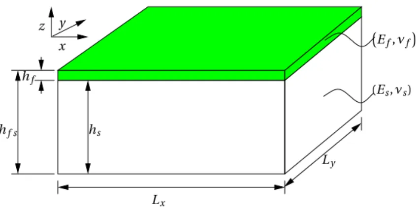
The domain has a rectangular shape, and the geometry of the considered problem is sketched in Figure 3. In the film, the material law is hyperelastic with a Saint Venant–Kirchhoff constitu-tive law, that is, a linear relation between the Green–Lagrange strain tensor and the second Piola– Kirchhoff stress tensor. Here, the substrate behavior is governed by small-strain isotropic elastic-ity. The numerical data are as follows: Lx= 1.5 mm, Ly= 1.5 mm, hf = 10−3mm, hs f = hs+ hf =
0.1 mm, Ef = 1.3 × 10⁵MPa, Ef = 1.8 MPa, νf = 0.3, and νs= 0.48, which characterize a film
Figure 3. Geometry and material data of the film–substrate system.
in [27] as well as the boundary conditions: A quarter of the domain is discretized with the cor-responding symmetry conditions, the vertical displacement is locked (uz= 0) along the bottom
face, and a compressive resultant stress is applied along the film faces x = 0 and x = Lx, where
the other components of the displacement are locked (uy= uz= 0). The applied uniaxial load λ
corresponds to the classical membrane stress, and it is measured in N/mm. The domain is dis-cretized by tetrahedra with P2 interpolation; it involves 100 rows of elements along its length and width, 5 rows through the thickness of the substrate and 1 through the film, which leads to 1.575 million degrees of freedom. The program is executed in parallel with MPI on four processors; it requires almost 55 GB of memory. The computation time is approximately 50 min for one ANM series and approximately 32 min for one Newton iteration. The cost of Newton iterations (64% of a series with 15 terms) is relatively large since the computation cost of the series is dominated by the cost of matrix factorization, which is a common feature of large-scale problems solved by the ANM [35, 36].
3.2. Computation without correction
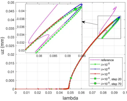
A reference result involving more than 280 steps is computed by the method from Section 2, which is discussed further. First, one tries to assess the behavior of the ANM algorithm without any correction. Hundred ANM steps are computed with various values of the accuracy parameter (δ = 10−3, 10−5, 10−6, 10−8). The first bifurcation point (λ ' 0.048 N/mm) is detected in the four cases, but the path-following technique fails very rapidly with the largest value (δ = 10−3). The results with other values ofδ can be analyzed with the naked eye from the curves λ–uzin Figure 4.
The response seems quasi-perfect for the smallest values (δ = 10−6, 10−8), while it deviates slightly
from the reference in the caseδ = 10−5.
However, response curves are not regarded as sufficient to assess the accuracy of numerical solutions of PDEs. They have to be characterized by the smallness of the residual (i.e., the L2 -norm of the residual vector), say a residual lower than 10−2or 10−3, as required within industrial
computer codes. In the case of intricate responses as the reference curve of Figure 4, a much smaller tolerance has to be required. In this paper, we prescribe a limit of 10−5for the sake of security. The evolution of the residual along the path is plotted in Figure 5, and one sees that this precision cannot be ensured for 100 steps irrespective of the tolerance (10−2or 10−5). Even for the smallest parameterδ = 10−8, the number of steps without correction is lower than 30 for a
tolerance of 10−5and lower than 50 for a tolerance of 10−2. Clearly, correction phases are required to achieve 100 secure continuation steps.
Figure 4. Response curve for load–displacement obtained with 100 ANM steps without correction and for various values of the accuracy parameter δ. The displacement uz is
chosen at the center of the film. The reference curve is obtained using the full algorithm from Section 2 by using 281 steps.
Figure 5. Evolution of the residual for 100 steps without correction and for various values of the accuracy parameterδ. The reference curve is computed by convergence acceleration, step adjustments, and Newton corrections.
3.3. Computation with corrections
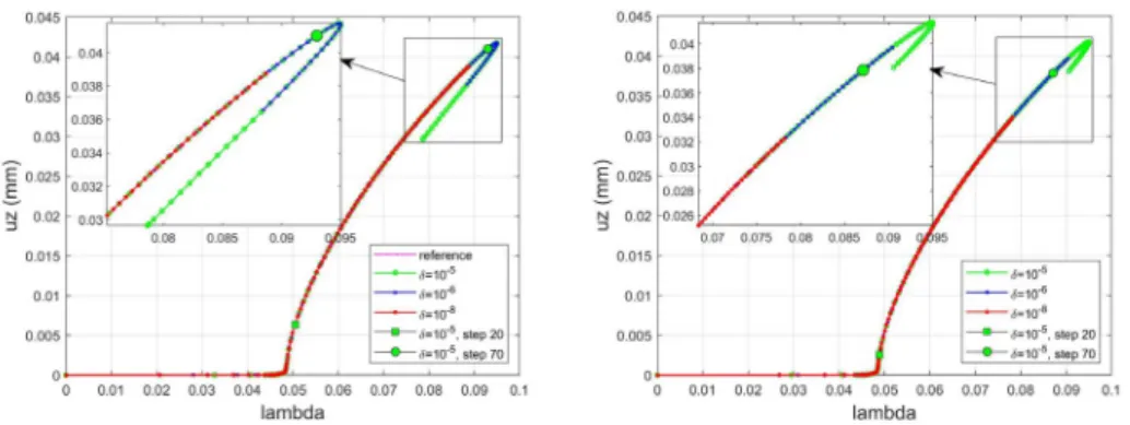
The same benchmark, that is, 100 ANM steps for the film–substrate problem described in Sec-tion 3.1, is discussed by applying two computaSec-tional strategies detailed in SecSec-tion 2. The
sim-Figure 6. Response curves for load–displacement obtained with 100 steps with correction for various values of the accuracy parameterδ. The displacement uzis chosen at the center
of the film. Curves with step-length adjustment (right) and without step-length adjustment (left).
plest strategy, referred to as the pure Newton corrector, enforces corrections as soon as the resid-ual is greater than²1= 10−5. The algorithm in Figure 2 defines another accuracy parameter²2
(here,²2= 10−6), which is a type of accuracy target: When possible, one tries to start each step
within this level of accuracy. The second strategy, referred to as the full algorithm, aims to reduce the number of correction phases. First, by applying convergence acceleration phases, a sequence of seven vectors (Vn= Un(a)) is accelerated by MMPE. The projection vectors Ynare
orthogonal-ized (i.e., Yn= V∗n); see Section 2.2.
A number of calculations are achieved, especially with several values of the ANM accuracy parameterδ (cf. (1)). The correction strategies prove to be very reliable: The residual always remains within the chosen limit²1= 10−5. The number of correction phases per step is limited
to one, rarely two. This efficiency is due to the quadratic convergence of the corrector and to the rather good accuracy of the chosen starting points of the correction phases. The total number of Newton corrections according to the parameterδ is presented in Table 1. This number is rather large; the best results are in the range 74–81, which means approximately three corrections for four ANM steps. Therefore, there are many corrections considering the hope of obtaining only sparse corrections, but it seems that this is the price of reliability in this difficult example. With the aforementioned computational costs, these 75 corrections correspond to an extra cost of 48%, which could be reduced in future studies by using various correction techniques, for instance as in [12] or in [37]. The computed response curves are plotted in Figure 6 for various values ofδ and for the chosen procedure. Of course, the size of the prediction steps is larger whenδ increases and it is smaller when the reduction technique from Section 2.3 is applied, but the effect of these changes in step size remains rather minor.
In fact, two very different behaviors of the algorithm are observed. For the first 20 steps, no correction is needed; the convergence acceleration method increases the accuracy and often increases the step size (i.e., r > 1). After the 20th step, a correction is required at almost every step, and the convergence acceleration becomes much less efficient.
A further look at the convergence acceleration brings out a rather common behavior of the algorithm beyond the 20th step. A typical example (δ = 10−5, step 70) is detailed in Table 2. The accuracy before MMPE is rather good at the first trial points (r = 0.7, 0.8) with a residual of the order of 10−3, but the convergence acceleration does not improve these solutions. For
r ≥ 0.9, this initial accuracy decreases when one moves away along the curve (residual of the
order of 10−1), but the convergence acceleration restores an accuracy of the order of 10−3. Step 70 is representative of the behavior of the prediction–correction algorithm observed in our
Table 1. Number of Newton corrections for 100 steps according to the accuracy parame-terδ
δ 10−5 10−6 10−8
Pure Newton 152 92 74 Full algorithm 81 79 74
The full algorithm includes convergence acceleration, step-length adaptation, and Newton correction(s). The required accuracy is²1= 10−5. The algorithm “pure Newton” (first line)
does not include convergence acceleration nor step adjustment. Table 2. Convergence acceleration by MMPE: a typical example
r 0.7 0.8 0.9 1 1.1 1.2 1.3
Before MMPE 0.0028 0.008 0.03 0.09 0.29 0.9 2.6 After MMPE 0.0034 1.1 0.007 0.005 0.004 0.004 0.004
The residuals before and after the application of MMPE are presented. Seven starting points
U(r amax), r ∈ [0.7,1.3] are considered. Step 70 with the full algorithm and δ = 10−5.
calculations. In the caseδ = 10−5, the first 19 steps work without correction and the convergence
acceleration by MMPE is efficient. In 12 steps out of 19, either Newton phases are avoided or the step is lengthened thanks to the use of MMPE. The subsequent steps are quite different because there is a Newton correction (and only one) at each of these steps, and the contribution of MMPE is much less effective. Indeed, if the shortest step lengths are considered (r = 0.7), the convergence acceleration never improves significantly the accuracy and the residual does not generally decrease. Typically, the residual goes from 10−3to 10−2or 10−3. On the contrary, the convergence acceleration is very efficient for the largest step lengths (r = 1.3) at least from steps 20 to 80. Three orders of magnitude are gained by MMPE from steps 20 to 70 and two orders for the next 10 steps. The residual passes typically from 1 to 10−3because of MMPE. Moreover, the Newton correction works well with a single iteration per step, and this always leads to residuals lower than 7 × 10⁻⁷and even to 10−8in 80% of the steps.
In brief, the introduction of correction phases permits us to build a very reliable procedure. The computation cost is increased by 48% compared to the computation without corrections; but the latter is incorrect. We suspect that the efficiency could be still improved but with slightly more intricate procedures.
3.4. Comments about the physics of axially compressed film–substrate systems
Finally, let us describe the evolution of the wrinkling pattern associated with the previously obtained response curves. Xu et al. [27] simulated the same benchmark by shell-volume finite elements but only up to uz/hf = 9. In this paper, a reference solution is established in Figure 4 by
computing 281 ANM steps using the full algorithm withδ = 10−6, convergence acceleration, step adjustments, and Newton corrections, ensuring high accuracy with a residual lower than 10−5at
each step.
Several turning points are observed along this curve. The first is located at uz/hf = 40, λ '
2λbif. The pattern evolution between the bifurcation point and the first turning point is
repre-sented in Figure 7. One observes a classical sinusoidal pattern just after the bifurcation that is quite perfectly periodic; see the left part of Figure 7. The bifurcation loadλbif' 0.05 and the
bifurcation mode are approximately the same as those in [27]. Next, the last wrinkle near the boundary develops more rapidly, highlighting a type of localization near the boundary (right part
Figure 7. 3D view of the deformed film just after bifurcation (step 20, Figure 4) and before the first turning point (step 70, Figure 4).
of Figure 7). This feature may be considered as a precursor of the appearance of a ridge (cf. [38]), but the chosen constitutive law does not permit us to go further.
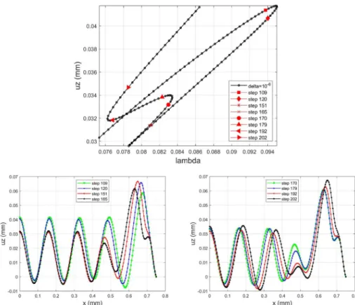
The multiple turning points occurring in this response curve do not favor the calculation by a path-following algorithm. The underlying physical phenomenon is not fully clear, but this is often associated with the appearance or disappearance of wrinkles [39, 40]. In the present case (see Figure 8), there are initially five wrinkles. Furthermore, the observed evolution brings out a tendency to pass from five to four wrinkles, the full story being slightly more intricate. First, close to the second turning point (step 151; Figure 8, left), a mini-wrinkle develops near the boundary, which pushes the other wrinkles to the left. At the same time, the amplitude of the fourth wrinkle decreases, and it seems that this wrinkle disappears when the top and bottom peaks coincide. Next, the evolution continues. Figure 8 (right) shows a further decrease in the fourth wrinkle and a disappearance of the mini-wrinkle near the boundary. If the third and fourth wrinkles shrink and tend to coincide, they will never fully merge during the 281 steps of this computation (Figure 8). Thus, in the last part of the response curve, one observes that two wrinkles coincide incompletely. It is remarkable that the three wrinkles in the center evolve together, with the loss of periodicity remaining located near the boundary.
4. Conclusion
Even if the paper mainly deals with numerical techniques, some interesting results have been also obtained about a basic benchmark for the wrinkling of the film–substrate system. The response curves obtained involve several hysteresis loops in the range uz/hf ' 40, which corresponds to
the growth of a single wrinkle near the boundary and to the unfinished disappearance of one wrinkle during the loading process. The authors are aware that the chosen 3D finite element model is not optimal for simulating a thin stiff film and that a shell element, possibly associated with a Winkler foundation, would be more efficient as shown in [27, 32]. This application of the ANM has led to a large-scale numerical model as in [35, 36].
The numerical techniques discussed here are from the field of ANM, which relies on the computation of the Taylor series with respect to a path parameter. It appears clearly that a simple chaining of the Taylor series leads to a progressive loss of accuracy when one has to chain many steps. Thus, correction phases based on the Riks–Newton technique are in-cluded, and this simple change ensures very secure computations with extremely high accu-racy. Hence, a path-following technique, thus modified, is efficient and very reliable for simu-lating wrinkling phenomena, while many authors prefer pseudo-dynamic procedures. This sim-ple prediction–correction method has been comsim-pleted using two inexpensive techniques: a
con-Figure 8. Mode evolution between the first and fourth turning points. Top figure: response curve between steps 100 and 220. Symmetry boundary conditions are applied at the left end point x = 0, while x = 0.75 is the boundary of the system. Evolution of the profile between steps 109 and 165 (left) and between steps 170 and 202 (right). The main phenomenon is the unfinished disappearance of two wrinkles near the boundary, while the wrinkling remains approximately uniform at the center.
vergence acceleration technique called MMPE and a step-length adaptation based on residuals. The number of Newton iterations per step observed in the test is generally limited to one or zero, but we did not succeed in chaining many steps without correction so that the price of reliability is approximately seven Newton iterations for 10 steps and an extra cost of 48% in computation time. It is likely that this cost could be reduced by using more advanced correction methods [12, 37]. As regards the convergence acceleration, its cost is negligible. Furthermore, it improves accuracy and reduces the number of correction phases but only in a sporadic manner. It is possible that this acceleration technique could also be improved.
Acknowledgment
The authors acknowledge the support of the French government through the National Research Agency ANR (LabEx DAMAS, Grant No. ANR-11-LABX-0008-01).
References
[1] B. Cochelin, N. Damil, M. Potier-Ferry, Méthode asymptotique numérique, Hermes Lavoisier, Paris, 2007.
[2] N. Damil, M. Potier-Ferry, “A new method to compute perturbed bifurcation: Application to the buckling of imperfect elastic structures”, Int. J. Eng. Sci. 26 (1990), p. 943-957.
[3] J. M. T. Thompson, A. C. Walker, “The non-linear perturbation analysis of discrete structural systems”, Int. J. Solids
Struct. 4 (1968), p. 757-768.
[4] A. K. Noor, J. M. Peters, “Tracing post-limit-point paths with reduced basis technique”, Comput. Methods Appl. Mech.
Eng. 28 (1981), p. 217-240.
[5] E. Riks, “Some computational aspects of the stability analysis of nonlinear structures”, Comput. Methods Appl. Mech.
Eng. 47 (1984), p. 219-259.
[6] B. Cochelin, N. Damil, M. Potier-Ferry, “The asymptotic-numerical method: an efficient perturbation technique for non-linear structural mechanics”, Revue Européenne des Éléments Finis 3 (1994), p. 281-297.
[7] B. Cochelin, C. Vergez, “A high order purely frequency-based harmonic balance formulation for continuation of periodic solutions”, J. Sound Vib. 324 (2009), p. 243-262.
[8] E. H. Boutyour, H. Zahrouni, M. Potier-Ferry, M. Boudi, “Bifurcation points and bifurcation branches by asymptotic-numerical method and Padé approximants”, Int. J. Numer. Methods Eng. 60 (2004), p. 1987-2012.
[9] W. Aggoune, H. Zahrouni, M. Potier-Ferry, “Asymptotic numerical methods for unilateral contact”, Int. J. Numer.
Methods Eng. 68 (2006), p. 605-631.
[10] B. Cochelin, “A path-following technique via an asymptotic-numerical method”, Comput. Struct. 53 (1994), p. 1181-1192.
[11] B. Cochelin, N. Damil, M. Potier-Ferry, “Asymptotic-Numerical Method and Padé approximants for non-linear elastic structures”, Int. J. Numer. Methods Eng. 37 (1994), p. 1187-1213.
[12] H. Lahmam, J. M. Cadou, H. Zahrouni, N. Damil, M. Potier-Ferry, “High order predictor-corrector algorithms”, Int. J.
Numer. Methods Eng. 55 (2002), p. 685-704.
[13] G. A. Baker Jr, P. Graves-Morris, Padé Approximants: Basic Theory, Encyclopedia of Mathematics and its Applications, vol. 13, Addison-Wesley, New York, 1996.
[14] A. Najah, B. Cochelin, N. Damil, M. Potier-Ferry, “A critical review of asymptotic numerical methods”, Arch. Comput.
Methods Eng. 5 (1998), p. 3-22.
[15] A. Elhage-Hussein, M. Potier-Ferry, N. Damil, “A numerical continuation method based on Padé approximants”, Int.
J. Solids Struct. 37 (2000), p. 6981-7001.
[16] S. Nezamabadi, H. Zahrouni, J. Yvonnet, “Solving hyperelastic material problems by asymptotic numerical method”,
Comput. Mech. 47 (2011), p. 77-92.
[17] Y. Guevel, E. H. Boutyour, J. M. Cadou, “Automatic detection and branch switching methods for steady bifurcation in fluid mechanics”, J. Comput. Phys. 230 (2011), p. 3614-3629.
[18] G. A. Baker Jr, “Defects and the convergence of Padé approximants”, Acta Appl. Math. 61 (2000), p. 37-52.
[19] M. Potier-Ferry, J. M. Cadou, “Basic ANM algorithms for path following problems”, Revue Européenne des Eléments
Finis 13 (2004), p. 9-32.
[20] C. Brezinski, “Convergence acceleration during the 20thcentury”, J. Comput. Appl. Math. 122 (2000), p. 1-21. [21] C. Brezinski, M. R. Zaglia, Extrapolation Methods: Theory and Practice, Elsevier, Amsterdam, 2013.
[22] K. Jbilou, H. Sadok, “Vector extrapolation methods, applications and numerical comparison”, J. Comput. Appl. Math.
122 (2000), p. 149-165.
[23] N. Damil, J. M. Cadou, M. Potier-Ferry, “Mathematical and numerical connections between polynomial extrapo-lation and Padé approximants: applications in structural mechanics”, Commun. Numer. Methods Eng. 20 (2004), p. 699-707.
[24] J. M. Cadou, L. Duigou, N. Damil, M. Potier-Ferry, “Convergence acceleration of iterative algorithms. Applications to thin shell analysis and Navier–Stokes equations”, Comput. Mech. 43 (2009), p. 253-264.
[25] E. Riks, “An incremental approach to the solution of snapping and buckling problems”, Int. J. Solids Struct. 15 (1979), p. 529-551.
[26] X. Chen, J. W. Hutchinson, “Herringbone buckling patterns of compressed thin films on compliant substrates”,
J. Appl. Mech. 71 (2004), p. 597-603.
[27] F. Xu, M. Potier-Ferry, S. Belouettar, Y. Cong, “3D finite element modeling for instabilities in thin films on soft substrates”, Int. J. Solids Struct. 51 (2014), p. 3619-3632.
[28] H. Mottaqui, B. Braikat, N. Damil, “Discussion about parameterization in the asymptotic numerical method: Appli-cation to nonlinear elastic shells”, Comput. Methods Appl. Mech. Eng. 199 (2010), p. 1701-1709.
[29] C. Brezinski, “Généralisations de la transformation de Shanks, de la table de Padé et de l’²-algorithme”, Calcolo 12 (1975), p. 317-360.
[30] R. Jamai, N. Damil, “Influence of iterated Gram-Schmidt orthonormalization in the asymptotic numerical method”,
C. R. Méc. 331 (2003), p. 351-356.
[31] Z. Y. Huang, W. Hong, Z. Suo, “Nonlinear analyses of wrinkles in a film bonded to a compliant substrate”, J. Mech.
Phys. Solids 53 (2005), p. 2101-2118.
[32] M. Lavrenˇciˇc, B. Brank, M. Brojan, “Multiple wrinkling mode transitions in axially compressed cylindrical shell-substrate in dynamics”, Thin-Walled Struct. 150 (2020), article ID 106700.
[33] A. Cutolo, V. Pagliarulo, F. Merola, S. Coppola, P. Ferraro, M. Fraldi, “Wrinkling prediction, formation and evolution in thin films adhering on polymeric substrata”, Mater. Design 187 (2020), article ID 108314.
[34] F. Hecht, “New development in FreeFem++”, J. Numer. Math. 20 (2012), p. 251-265.
[35] M. Médale, B. Cochelin, “A parallel computer implementation of the Asymptotic Numerical Method to study thermal convection instabilities”, J. Comput. Phys. 228 (2009), p. 8249-8262.
[36] Y. Guevel, T. Allain, G. Girault, J. M. Cadou, “Numerical bifurcation analysis for 3-dimensional sudden expansion fluid dynamic problem”, Int. J. Numer. Methods Fluids 87 (2018), p. 1-26.
[37] J. M. Cadou, M. Potier-Ferry, “A solver combining reduced basis and convergence acceleration with applications to non-linear elasticity”, Int. J. Numer. Methods Biomed. Eng. 26 (2010), p. 1604-1617.
[38] Y. Cao, J. W. Hutchinson, “Wrinkling phenomena in neo-Hookean film/substrate bilayers”, J. Appl. Mech. 79 (2012), article ID 031019.
[39] W. Wong, S. Pellegrino, “Wrinkled membranes III: numerical simulations”, J. Mech. Mater. Struct. 1 (2006), p. 63-95. [40] C. G. Wang, L. Lan, H. F. Tan, “Secondary wrinkling analysis of rectangular membrane under shearing”, Int. J. Mech.