HAL Id: hal-02106342
https://hal-amu.archives-ouvertes.fr/hal-02106342
Submitted on 22 Apr 2019
HAL is a multi-disciplinary open access
archive for the deposit and dissemination of
sci-entific research documents, whether they are
pub-lished or not. The documents may come from
teaching and research institutions in France or
abroad, or from public or private research centers.
L’archive ouverte pluridisciplinaire HAL, est
destinée au dépôt et à la diffusion de documents
scientifiques de niveau recherche, publiés ou non,
émanant des établissements d’enseignement et de
recherche français ou étrangers, des laboratoires
publics ou privés.
Heterogeneous and rate-dependent streptavidin–biotin
unbinding revealed by high-speed force spectroscopy and
atomistic simulations
Felix Rico, Andreas Russek, Laura Gonzalez, Helmut Grubmüller, Simon
Scheuring
To cite this version:
Felix Rico, Andreas Russek, Laura Gonzalez, Helmut Grubmüller, Simon Scheuring. Heterogeneous
and rate-dependent streptavidin–biotin unbinding revealed by high-speed force spectroscopy and
atom-istic simulations. Proceedings of the National Academy of Sciences of the United States of America
, National Academy of Sciences, 2019, 116 (14), pp.6594-6601. �10.1073/pnas.1816909116�.
�hal-02106342�
Heterogeneous and rate-dependent streptavidin–biotin
unbinding revealed by high-speed force spectroscopy
and atomistic simulations
Felix Ricoa,1,2, Andreas Russekb,1, Laura Gonzálezc, Helmut Grubmüllerb,2, and Simon Scheuringd,e,2
aLaboratoire Adhésion et Inflammation (LAI), Aix-Marseille Université, CNRS, INSERM, 13009 Marseille, France;bDepartment of Theoretical and
Computational Biophysics, Max Planck Institute for Biophysical Chemistry, 37077 Göttingen, Germany;cDepartment of Electronics, Universitat de Barcelona,
08028 Barcelona, Spain;dDepartment of Anesthesiology, Weill Cornell Medical College, New York, NY 10065; andeDepartment of Physiology and
Biophysics, Weill Cornell Medical College, New York, NY 10065
Edited by Taekjip Ha, Johns Hopkins University, Baltimore, MD, and approved February 21, 2019 (received for review October 4, 2018)
Receptor–ligand interactions are essential for biological function and their binding strength is commonly explained in terms of static lock-and-key models based on molecular complementarity. However, detailed information on the full unbinding pathway is often lacking due, in part, to the static nature of atomic structures and ensemble averaging inherent to bulk biophysics approaches. Here we combine molecular dynamics and high-speed force spec-troscopy on the streptavidin–biotin complex to determine the binding strength and unbinding pathways over the widest dynamic range. Experiment and simulation show excellent agreement at overlapping velocities and provided evidence of the unbinding mechanisms. During unbinding, biotin crosses multiple energy bar-riers and visits various intermediate states far from the binding pocket, while streptavidin undergoes transient induced fits, all vary-ing with loadvary-ing rate. This multistate process slows down the tran-sition to the unbound state and favors rebinding, thus explaining the long lifetime of the complex. We provide an atomistic, dynamic picture of the unbinding process, replacing a simple two-state pic-ture with one that involves many routes to the lock and rate-dependent induced-fit motions for intermediates, which might be relevant for other receptor–ligand bonds.
high-speed atomic force microscopy
|
high-speed force spectroscopy|
receptor/ligand bonds|
single molecules|
molecular dynamics simulationsR
eceptor/ligand bonds are at the core of almost everybi-ological process. The early lock-and-key model including possible conformational changes of the binding partners is commonly accepted to describe the affinities and kinetic rates of receptor/ligand complexes and is mainly based on molecular complementarity pictures from static structural data (1, 2). Over the past decades, an impressive amount of knowledge has been accumulated on the structural and energetic determinants of bound states, thus enabling the increasingly successful rational design of nanomolar binders for therapy as well as the quanti-tative prediction of binding processes and free energies from atomistic simulations (3). While protein folding and unfolding are thought to follow a multiplicity of pathways, the very mecha-nism of binding or unbinding of receptor/ligand complexes remains less investigated and is generally described by a simple two-state model, or by the lock-and-key analogy. Moreover, little is known on how the (un)binding dynamics is governed by the underlying microscopic processes—despite being key to a quantitative understanding of receptor–ligand complexes. Progress is mostly hampered by the lack of structural and thermodynamic information of the transient ligand/receptor conformations during unbinding, even for extensively studied systems such the complex formed by streptavidin (SA) and the small molecule biotin (b, vitamin H), one of the strongest noncovalent bonds known in nature.
SA forms the b-binding pocket with an eight-stranded, anti-parallel beta-barrel capped by loop 3–4 (Fig. 1A). In the native, tetrameric SA form, loop 7–8 from an adjacent monomer provides
a closing lid to the pocket (4). b binds by forming an intricate and extensive network of hydrogen bonds with polar residues of SA (4, 5). Its high affinity (Kd∼ 10−13M) and long lifetime (τ ∼ 10 d,
koff∼ 10−6s−1) (6–9) make the SA/b system extensively used in
biotechnology and biophysics. Dynamic forced disruption of the SA–b complex by atomic force microscopy (AFM) and other techniques pioneered single-molecule biomechanics (10–13) and provided estimates of the distance xβto the unbinding transition state and the intrinsic bond lifetime (13–15). Despite its seeming simplicity, AFM (11, 16–19), optical tweezers (20), and bio-membrane force probe (10, 21) experiments of SA/b unbinding have reported dissimilar results, suggesting an impressive com-plexity and heterogeneity in the unbinding pathway (SI Appendix). Furthermore, the results from single-molecule studies were incom-patible with ensemble bond-lifetime measurements (6).
Although recent experimental developments accessing the microsecond timescale have shed light into the complexity of single-molecule transition paths of protein and nucleic acid (un) folding (22–25), the amount of transient structural information extracted from single-molecule experiments is rather limited.
Significance
Protein–ligand interactions are commonly described in terms of a two-state or a lock-and-key mechanism. To provide a more detailed and dynamic description of receptor–ligand bonds and their (un)binding path, we combined high-speed force spec-troscopy and molecular dynamics simulations to probe the prototypical streptavidin–biotin complex. The excellent agree-ment observed, never used for force-field refineagree-ment, provides the most direct test of the “computational microscope.” The so-far largest dynamic range of loading rates explored (11 decades) enabled accurate reconstruction of the free-energy landscape. We revealed velocity-dependent unbinding pathways and in-termediate states that enhance rebinding, explaining the long lifetime of the bond. We expect similar behavior in most receptor– ligand complexes, implying unbinding pathways governed by transient, timescale-dependent induced fits.
Author contributions: F.R., A.R., L.G., H.G., and S.S. designed research; F.R., A.R., L.G., and H.G. performed research; F.R., A.R., and H.G. analyzed data; and F.R., A.R., H.G., and S.S. wrote the paper.
The authors declare no conflict of interest. This article is a PNAS Direct Submission.
This open access article is distributed underCreative Commons Attribution-NonCommercial-NoDerivatives License 4.0 (CC BY-NC-ND).
1F.R. and A.R. contributed equally to this work.
2To whom correspondence may be addressed. Email: [email protected], hgrubmu@
gwdg.de, or [email protected].
This article contains supporting information online atwww.pnas.org/lookup/suppl/doi:10. 1073/pnas.1816909116/-/DCSupplemental.
www.pnas.org/cgi/doi/10.1073/pnas.1816909116 PNAS Latest Articles | 1 of 8
BIOPHYSICS
AND
COMPUTATION
AL
Therefore, most structural knowledge on unbinding/unfolding processes has been derived from atomistic simulations that were often limited to short timescales inaccessible to experiments and therefore not rigorously validated (24–28). Thus, today, a direct relationship between the energy landscape and the dynamic structural details of these seemingly simple biomolecular pro-cesses is missing. As a result, it is still unclear (i) how b precisely outlives days and unbinds under load, (ii) how and where b is located at the point of rupture and how the respective interme-diates are stabilized, (iii) if there is only one or possibly several unbinding pathways, and if so, (iv) to what extent the unbinding paths change with loading rate. Here we address these questions by combining high-speed force spectroscopy (HS-FS) and fully at-omistic simulations to observe b unbinding from SA over 11 de-cades of loading rates. We show that the unbinding pathway of the small molecule b from SA is much more complex than a “key that leaves a lock” and reveal a multitude of pathways and intermediate binding sites far from the binding pocket, similar to the various pathways and intermediate states of protein (un)folding.
For the HS-FS experiments we used microcantilevers func-tionalized with b to probe the force required to rupture indi-vidual SA–b bonds at various loading rates (Fig. 1A, Left). The use of microcantilevers with response time of∼0.5 μs and reading out the reflected laser beam at 0.05 μs (high sampling rates up to 20 million samples per s) allowed tracking the cantilever position while pulling at velocities up to∼30,000 μm/s, almost an order of magnitude faster than previous HS-FS measurements and about 1,000 times faster than conventional AFM FS measurements (11, 19, 29). All atom steered molecular dynamics (SMD) simulations
precisely mimicked the experimental setup by using the fully sol-vated tetrameric structure of SA [Protein Data Bank (PDB) ID code 3RY2 (4)] and by pulling b using two springs in series, using the worm-like chain (WLC) model describing the PEG linker and a linear spring for the cantilever, whose end was moved at con-stant velocity (Fig. 1A, Right andMovies S1–S3). The overall ap-plied pulling velocities ranged from 0.05 μm/s to 30,000 μm/s in HS-FS experiments (Fig. 1B) and from 1,000 μm/s to 5 × 1010μm/s
in SMD simulations (Fig. 1C), resulting in a combined range of loading rates from∼100 pN/s to ∼1013pN/s, covering 11 decades.
Importantly, the wide experimental dynamic range up to such fast rates, together with recent simulation advances (30, 31), allowed direct overlap and comparison with in silico simulation loading rates over an entire decade between 108and 109pN/s (Fig. 2 and SI Appendix).
The measured force curves showed a characteristic curve of increasing force due to stretching of the flexible PEG linker (Fig. 1), signature of the specificity of the interaction (32) (Materials and Methods). Fig. 2 shows the dynamic force spectrum obtained both from the most probable rupture forces at each loading rate (in piconewtons per second) in the experiments (circles) as well as from the average rupture force of 10 to 20 simulations per loading rate (triangles). At the overlapping loading rates, rupture forces from experiments and simulations agreed very well, thereby providing independent validation for the MD simula-tions. At the lowest loading rates, from∼102pN/s up to∼106pN/s
(∼103μm/s pulling velocity), rupture forces increased almost
lin-early with the logarithm of the loading rate, indicating one single dominant barrier in this loading rate regime. At faster loading rates, steeper slopes are observed. This behavior has been inter-preted before in several ways: (i) multiple transition barriers along the 1D energy landscape, inner barriers becoming dominant at high loading rates and outer barriers, at low rates (10, 19); (ii) force-induced shortening of the distance to the transition state (14, 33); and (iii) a transition from a thermally activated to a so-called deterministic regime (15, 24, 34). Another possible cause (iv) might be that the cantilever response affects the force spectrum for pulling timescales shorter than the cantilever re-sponse time (35, 36). Actually, previous experiments using devices
A
B
C
Fig. 1. High-speed and MD force spectroscopy of SA–b unbinding. (A, Left) HS-FS setup. SA agarose beads (Top Left) were immobilized on the sample surface while b was covalently attached to the microcantilever (Bottom Left) through a PEG linker (contour length∼10 nm). (A, Right) MD simulations setup and the SA–b tetramer used in the MD simulations with labeled loops 3– 4 and 7–8 (PDB ID code 3RY2). (B) Experimental force–distance traces at ve-locities from 1 μm/s to 30,556 μm/s revealing bond rupture events using AC7 (top curve) and AC10 cantilevers (bottom curves). The stretching profile of the experimental curves was the result of stretching the PEG linker and deforming the agarose bead to which SA was linked. (C) Force–extension traces from the MD simulations at retraction velocities from 1,000 μm/s to 2 × 10⁶
μm/s.
Fig. 2. Dynamic force spectrum of SA/b unbinding. Most probable rupture forces (± SEM) from HS-FS experiments (circles, using regular AC10 and fast AC7 cantilevers, cyan and magenta, respectively) and MD simulations (tri-angles). The blue line represents a Brownian dynamics fit to the whole force spectrum. (Inset) The resulting equilibrium free-energy landscape is shown as a blue line, which revealed two transition barriers (with parameters D = 4 × 10⁷nm2
/s, ΔG1= 17 kBT, ΔG2= 21 kBT, xβ1= 0.19 nm, and xβ2= 0.44 nm) and
a possible intermediate state between the two (blue dashed line). The red dashed line sketches a third, outer barrier (Fig. 3 and text), which cannot be extracted from the dynamic force spectrum.
with a dynamic response slower than HS-FS cantilevers (response time τc∼ 50 to 500 μs, effective diffusion constant Dp∼ 102to 103
nm2/s, compared with τ
c∼ 0.5 μs, Dp∼ 105nm2/s) have reported a
marked slope increase at loading rates∼104pN/s (10, 16, 19, 29),
while our first slope increase occurred at∼106pN/s. This suggests
that this possible effect (iv) is reduced using HS-FS microcanti-levers, which allows orders of magnitude faster loading rates be-fore this possible effect may appear.
By virtue of the broad range of loading rates covered here, the combined dynamic force spectrum contains more information on the free-energy landscape of unbinding than has been accessible before. As detailed below, all three possible explanations (i–iii) seem to contribute to the shape of the energy landscape. In particular, single-barrier models did not describe the entire dy-namic force spectrum satisfactorily, supporting the presence of a more complex energy landscape with multiple barriers (14, 15, 34, 36, 37) (SI Appendix, Fig. S7). To avoid approximations in-herent to analytic theories, we instead performed Brownian dy-namics simulations using a more complex energy landscape with two barriers and varied the shape and height of these barriers (Fig. 2, Inset; see alsoSI Appendix) until the best agreement with the dynamic force spectrum (blue line in Fig. 2) was obtained. Importantly, this free-energy landscape explains both experiment and simulation over the whole 11 decades of loading rates. The energy landscape has a first (inner)∼17 kBT barrier at 0.19 nm,
which determines the force spectrum slope at loading rates faster than 106pN/s, and a second∼21 k
BT unbinding barrier further
out at 0.44 nm (Fig. 2, Inset, blue line). The longer rupture length of the second barrier, which becomes rate-limiting only at lower unbinding rates, gives rise to the shallower slope at loading rates below 106pN/s. We note that the MD simulations suggest
inter-mediate states (i.e., a well between these two barriers, sketched as a dashed blue line in the inset), which, however, cannot be extracted (or ruled out) by analyzing the force spectrum alone (33). Also, a third unbinding barrier further out at distances larger than 0.44 nm (indicated by the dashed red line in the inset) is seen in our experimental force curves and MD simulations and will be discussed below. However, in the force spectrum this barrier would only become kinetically dominant at lower loading rates than probed in our HS-FS experiments and is therefore not seen. According to the Bell–Evans theory, one would expect two distinct slopes in the force spectrum, corresponding to the two kinetically relevant unbinding barriers (13). In our dynamic force spectrum, we observe, however, a rather continuous slope in-crease up to 1011pN/s attributed to a force-induced shortening
of the rupture length of these two barriers, as predicted by the-ories that take the shape of the barriers into account (14, 36). Finally, the slight deviation of the Brownian dynamics (BD) curve at very fast loading rates >1011pN/s may indicate a
tran-sition from a diffusion-dominated (Bell–Evans regime) to a de-terministic regime (15, 34). For SA–b, this critical loading rate (F· >> Fc cDxβ−2)∼1011pN/s (or∼1010nm/s) is orders of
mag-nitude faster than that observed in previous HS-FS experiments of titin unfolding (∼107 pN/nm, ∼106 nm/s) (24). This was
expected since the transition is supposed to emerge when the pulling rate is faster than the intrinsic time required for the complex to explore its energy landscape. This intrinsic time was (xβ2/D)∼ 0.2 ms for titin I91 but much shorter (∼1 ns) for SA/b,
which is reasonable given the less pronounced structural changes of the b molecule compared with partial titin domain unfolding. The MD unbinding simulations (>300 in total) provided structural information on the loading-rate-dependent unbinding paths. Fig. 3A shows the distribution of center of mass (COM) distances from all MD trajectories between the SA binding pocket, defined as the set of amino acids that interact with the bound b in the static crystal structure, and the b molecule. The peak at 0 nm represents the bound state followed by two con-secutive minima at∼0.25 nm and ∼0.5 nm. These values are
slightly left of the positions of the two barriers (∼0.19 nm and ∼0.44 nm) obtained from the BD fit of the force spectrum and suggest the COM distance as an appropriate reaction coordinate of unbinding. Interestingly, the peak between and to the right of these two minima suggests that, at least upon force application, one or several metastable states appear, as a result of the tilted energy landscape. Importantly, these metastable states will favor rebinding at sufficiently slow pulling rates (37, 38). The simula-tions show that most of the H-bonds between b and the SA binding pocket remain intact until b has moved∼0.15 nm toward the outside of the SA binding pocket. At the distance corre-sponding to the first barrier, the H-bonds between residues Ser27, Tyr43, Asn49, and Asp128 and the b, rather parallel to the pulling direction, rupture. Escape from the binding pocket oc-curs only after the second barrier at∼0.5 nm, where most of the remaining H-bonds between b and SA (mainly with residues Asn49, Tyr54, and Arg84) rupture (Fig. 4B andSI Appendix, Fig. S9). Notably, these H-bonds are nearly perpendicular to the unbinding direction (long axis of the binding pocket), which implies a shear force, and only simultaneous failure of all H-bonds lead to dissociation, with subsequent transient formation of a different H-bond network (SI Appendix, Fig. S9). A similar mechanism has been observed before as key to providing stability against forced protein unfolding (39, 40). Overall, the geometry of rupture and reconfiguration of the H-bond network between b and adjacent amino acids of the binding pocket seems to rep-resent the main determinants of the dynamic force spectrum in Fig. 2, described by the energy landscape with two barriers.
A
D
E
B
C
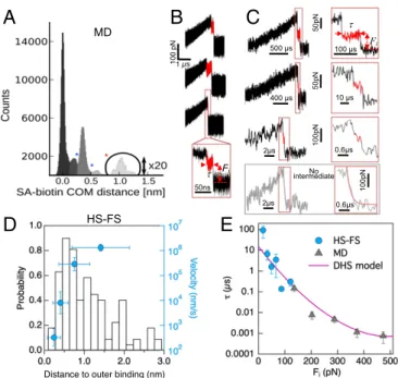
Fig. 3. Outer barrier. (A) Distribution of COM distances between SA and b for all MD trajectories during unbinding. The first two minima coincide with the barrier positions obtained from the Brownian dynamics simulations fit of the force spectrum in Fig. 2, Inset. (B) Examples of MD and (C, top three) HS-FS force–time curves showing outer binding. The lifetime and applied force of outer binding events was determined as shown (red lines) and described in Materials and Methods. The bottom curve shows an example for which no intermediate was observed. The red line shows an exponential fit with decay time∼0.28 μs. (D) Distribution of experimental distance to outer binding (left axis) and pulling velocity dependence of the average distance (blue, right axis). (E) Outer binding lifetime vs. applied force from HS-FS (circles) and MD simulations (triangles). The solid line shows the best fit to the force-dependent lifetime DHS model (14) with parameters τ0= 16 ± 7 μs, xβ=
0.16 ± 0.10 nm, and ΔG = 12 ± 6 kBT. This distance the outer barrier (xβ)
should be added to the position of the second barrier at xβ2= 0.60 nm in Fig.
2 (sketched as a dashed red line in the inset).
Rico et al. PNAS Latest Articles | 3 of 8
BIOPHYSICS
AND
COMPUTATION
AL
One might assume that linear extrapolation of the force spec-trum to zero force should yield a time scale similar to the spon-taneous SA–b unbinding off-rate koff∼10−6s−1 obtained from
bulk equilibrium experiments (7). However, as in previous single-molecule force experiments (10, 19) (SI Appendix), Fig. 2 would suggest a much faster off-rate of∼1 s−1. Notably, also the 21 k
BT
barrier (blue line in Fig. 2, Inset) in the unbinding energy land-scape is∼19 kBT lower than the calorimetric SA–b binding free
energy of ∼40 kBT (7). Further, a Kramers estimate using an
attempt frequency of 109s−1would also predict a∼1 s−1off-rate.
Whereas the end states of enforced and spontaneous unbinding are not the same and, hence, the respective (un)binding free-energy differences are not expected to fully agree, such a large discrepancy is unexpected. To reconcile forced and equilibrium unbinding, a third barrier located further out on the unbinding pathway should be present (as depicted in Fig. 2, Inset, red dashed line), as was speculated before from indirect evidence
(10, 21). Such a barrier would show up in a dynamic force spectrum at loading rates much lower than accessible to exper-iments (and certainly to simulations) and, therefore, remained so far unobserved. One would, however, expect to observe inter-actions between SA and b farther out of the binding pocket, as structural determinants of this barrier.
Indeed, our MD simulations revealed such interactions and corresponding intermediate states. In particular, the distribution of COM distances between the SA binding pocket and the b molecule displays a pronounced peak after the second minimum followed by smaller peaks at distances up to 1.5 nm (Fig. 3A and
SI Appendix). Detailed inspection of the individual MD trajec-tories showed as many as eight transient H-bonds (mainly to ASN49, GLU51, and TYR54) formed with b∼1 nm away from the binding pocket (Fig. 3A). Importantly, the force profiles (Fig. 3B) from these trajectories (∼15% of all trajectories) displayed adhesive interactions after and at a lower value than the main force peak and, therefore, these states are not seen in the dy-namic force spectrum. In these events, the force applied to b displays a drop due to the exit from the binding pocket and a subsequent intermediate force plateau with a final drop due to complete detachment. At the slowest MD velocities, this tran-sient unbinding state lasted up to several hundred nanoseconds, such that it should also be detectable using HS-AFM micro-cantilevers with submicrosecond resolution.
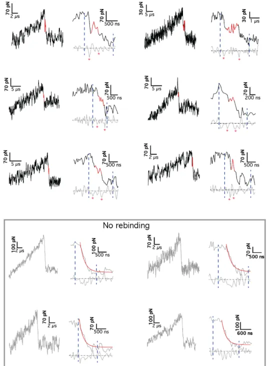
To test this hypothesis, we analyzed in further detail the in-dividual experimental force curves. Remarkably, we observed a similar signature in about 5% of the HS-FS unbinding events with a transient force plateau during the snap off of the canti-lever (Fig. 3C andSI Appendix, Figs. S5 and S6). These transient, microsecond-long events were observed over the full range of experimental loading rates and provide an experimental signa-ture of the transient outer states. The low occurrence of these events in HS-FS curves may be due to their short lifetime. Moreover, the distance from the force peak to the transient binding had an average value∼1 nm extending up to 3 nm (Fig. 3D), similar to the distances seen in the MD trajectories (Fig. 3A). Therefore, the combination of HS-FS and MD simulations of SA/b forced unbinding provided first direct experimental ev-idence and a structural description of an outer binding state that may be at the basis of the SA/b sturdiness.
The large number of experiments and simulations allowed us to characterize the average lifetime τ of these outer binding states. Fig. 3E shows that τ ranges from 0.001 μs to 100 μs for forces Fi
between 500 pN down to 20 pN (including MD and HS-FS data). Hence, excellent agreement between experiments and simulations is seen also in the time domain. The average lifetime decayed exponentially with force and can be described by a single barrier (14) of 12 kBT additional height with a rupture length of 0.16 nm
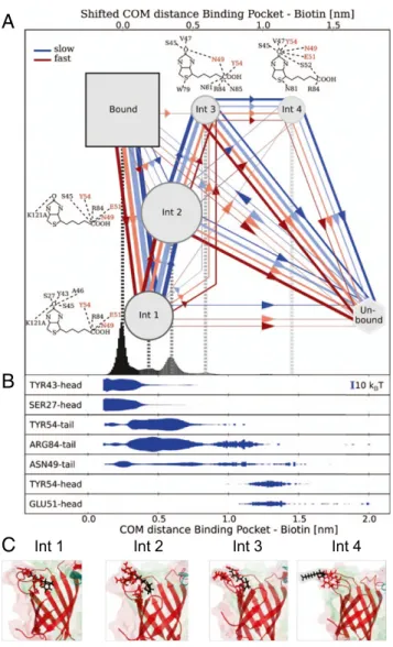
and, notably, of∼16-μs lifetime at zero force (Fig. 3D). This third barrier (red dashed line in Fig. 2, Inset) is located outside the second barrier (blue line), at a distance of 0.60 nm from the bound state (red line in Fig. 2, Inset) and adds a further step upward to the energy landscape toward the fully unbound state. This distance correlates with a minimum in the COM distance at ∼0.7 nm. Although the exact minimum preceding this outer barrier is dif-ficult to pinpoint, metastable states before this barrier are expected upon force application, as reflected from the peak in the COM distribution at∼0.6 nm. This barrier further slows down b unbinding by several orders of magnitude, thereby reconciling it with the observed slow equilibrium off-rate. The respective inter-actions between b and the outside of the binding pocket should favor rebinding events, in particular at low and zero forces. Although rare, back-and-forth fluctuations between intermediate states were actually observed in some of the MD trajectories (Fig. 4).
As shown in Fig. 3D, the experimental distance to the outer binding increased with the pulling velocity, suggesting that shorter jumps occur more often at slow pulling. This suggests that, although
A
B
C
Fig. 4. Dynamic multiplicity of SA–b unbinding pathways. (A) Bound and intermediate states with unbinding pathways observed during forced dis-sociation in MD trajectories. The line color reflects pulling velocity from slow (blue) to fast (red) and thickness reflects passage frequency. b molecular representations show overlays of the hydrogen bonds with SA residues for the four intermediate states. The amino acids with the strongest interme-diate interactions are labeled in red. (B) The energy of the H-bonds between b and the most important residues is shown below as a function of the COM distance. (C) Structural snapshots of the different intermediate states showing H-bonds between SA residues and b.
effectively described by a single barrier, the outer barrier may in-volve not only one but several intermediate states, not directly re-solved experimentally and with varying occupancies that depend on the pulling velocity. This notion is further supported by the various peaks observed in the COM distance outside of the binding pocket, which allowed characterizing the four most populated intermediate states (Int 1 through Int 4, Fig. 4A). Importantly, various unbinding paths were seen in the trajectories. The large number of atomistic simulations for each loading rate allowed us, finally, to study to what extent the observed unbinding pathways change with loading rate. Under high load, mainly two intermediate binding states (Int 1 and Int 2) are visited along the unbinding pathway. At lower loading rates, states Int 3 and Int 4, farther out, are also visited. Likely these, and even intermediates lying farther outside, provide a rugged funnel (41–43) for rebinding under equilibrium conditions.
Calculating the average energy of the H-bonds between b and individual amino acids in the binding pocket from all MD tra-jectories as a function of the b position (Fig. 4B andSI Appendix, Fig. S9) allowed us to extract structural snapshots of each in-termediate state (Fig. 4C). Whereas the inner inin-termediate states showed strongest interactions between the ureido moiety of b and residues Ser27, Tyr43, and Asp128, respectively, at later stages of unbinding other bonds, largely overlooked so far, become rele-vant, such as Arg84, Glu51, and Tyr54, at COM distances of up to 1.5 nm from the bound state (Fig. 4B). While SA modifications of these three residues have reported lower b affinity (6, 44, 45), they have not been expected to be involved in b binding due to their large separation from the binding pocket and their little contri-bution to the bound state, underscoring the impact of features along the unbinding path on binding kinetics.
One might speculate that SA has evolved in tetrameric form because it allows for even larger binding affinity due to inter-monomeric stabilization, with the 7–8 loop providing the key interprotomer interaction (5). To test this idea, we repeated our steered MD simulations using monomeric SA—which is difficult experimentally. As suggested before from high-loading-rate simulations on avidin–b unbinding (27), rupture forces of the monomer were systematically 10 to 20% lower than for the tet-ramer over the whole loading-rate range (SI Appendix, Fig. S8
and Movies S4–S6), thus further supporting this hypothesis. Closer structural analysis of the unbinding paths suggests that these reduced unbinding forces are due to (i) lacking inter-monomeric interactions [specifically to the 7–8 loop of the ad-jacent protomer (27)] and (ii) an increased heterogeneity of unbinding paths, the larger entropy of which further reduces the unbinding barrier.
Strikingly, the unbinding-rate-dependent heterogeneity and occupancies of intermediate states are accompanied by rate-dependent, nonequilibrium dynamics of the SA structure while b moves toward the unbound state. We observed induced-fit mo-tions (of the binding pocket and adjacent loops) outside the fully bound state, along the (un)binding path. As an example, loop 3– 4 switches between an open and a closed conformation during unbinding, depending on the distance between b and the binding pocket (SI Appendix, Fig. S10). These nonequilibrium confor-mational changes are more pronounced at slower loading rates, for which the loop has more time to fluctuate and equilibrate (SI Appendix, Fig. S10). Therefore, it should also occur in the AFM experiments as well as during spontaneous unbinding. This finding suggests that “induced fit” and other nonequilibrium con-formational changes of SA control not only the bound state but also the transient energetics and kinetics along the binding and un-binding paths, and in a loading-rate-dependent manner.
The combination of HS-FS and MD simulations at overlapping loading rates allowed us to obtain a dynamic and atomistic de-scription of a receptor–ligand unbinding process. Characterizing enforced SA/b unbinding over an unprecedentedly large range of loading rates enabled us to characterize large portions of the
underlying energy landscape, which would not have been acces-sible by one of the two methods alone. Notably, it also allowed for a most direct comparison between AFM experiment and MD simulation. The excellent agreement of rupture forces at over-lapping loading rates—an observable that has never been used for force field parameterization—underscores the predictive power of atomistic MD simulations.
Single-barrier theoretical models successfully describe the spec-trum over a wide range at high loading rates and serve to interpret our results (SI Appendix, Fig. S7). The fitted Bullerjahn–Sturm–Kroy (BSK) model predicts a transition toward the deterministic regime at rates ∼1011 pN/s only reached by MD simulations,
that may explain the change in slope at this loading rate (15). The recently developed Cossio–Hummer–Szabo (CHS) model, which described remarkably well the dynamic force spectros-copy, predicts instead a kinetically ductile regime described as gradual stretching and shortening of the distance to the tran-sition state under force before unbinding, which helps un-derstand the curvature observed at high loading rates (Fig. 2 andSI Appendix, Fig. S7). The low value, close to zero, of the unitless kinetic brittleness [μ ∼ 10−6;SI Appendix, Fig. S7(36)]
found for our spectrum is consistent with a ductile behavior for SA/b. Inclusion of the low-loading-rate regime requires multi-ple barriers (38), and the full dynamic force spectrum over 11 decades is only accurately described by BD simulations. Finally, outer barriers at distances beyond the energy landscape of Fig. 2 (Inset, blue line) would enhance rebinding and likely emerge in the force spectrum at loading rates lower than the ones explored in our work (but were detected as transient binding events in both HS-FS and SMD). Therefore, combi-nations of available analytical theories seem to be required to fully explain the force spectrum over the whole dynamic range, including a more refined description taking into account the dynamic nature of the energy landscape.
Our concerted approach revealed multiple unbinding path-ways and nonequilibrium conformational changes of the SA binding pocket dependent on loading rate, with a detailed de-scription of the pathway fluxes. In particular, outer intermediates were found that affect binding energetics and kinetics. Future combination of HS-FS and MD simulations will answer whether these proposed mechanisms found for SA/b are specific to this bond or—in our view more likely than not—a common feature of many receptor/ligand complexes and thus a general mechanism of regulating binding kinetics. If this were the case, the study of intermediates and their mechanism would be instrumental in improving the binding kinetics and specificity of drug-like com-pounds. Taken together, our results suggest that the current static picture based on the bound state may need to be extended in terms of many routes to (un)binding as well as multiple, transient, and nonequilibrium-induced fits, resembling a combination lock, where several intermediate positions have to be visited for final release. The development of theoretical models taking into ac-count the dynamic nature of the energy landscape will help us better understand biological bonds.
Materials and Methods
HS-AFM Tips and Sample Preparation. SA-coated 4% agarose beads (Sigma) were immobilized on the sample surface by embedding them in a thin agarose layer. b was covalently attached to the cantilever through a PEG linker (stretched length∼10 nm; Fig. 1A). Briefly, HS-AFM (AC10DS and AC7) cantilevers (Olympus) were rinsed with acetone for 10 min, plasma-cleaned for 5 min in O2, and immersed in a solution of 10 to 20 mg/mL
silane-PEG-biotin (1 kDa; Nanocs Inc.) in ethanol/water (95/5). After 2 h incubation, cantilevers were rinsed with ultrapure water and stored at 4 °C until use. HS-FS Measurements. HS-FS measurements were carried out on an HS-AFM (RIBM) featuring a high-speed acquisition board system (PXI; National Instru-ments) to control the z-movement and acquire force curves at sampling rates up to 20 MS/s. Two types of cantilevers with submicrosecond time response
Rico et al. PNAS Latest Articles | 5 of 8
BIOPHYSICS
AND
COMPUTATION
AL
and small viscous damping were used: AC10 cantilevers with 600-kHz resonance frequency in liquid, 0.1 N/m spring constant, quality factor of 0.9, and 0.09 pN·μm−1·s−1viscous coefficient; and shorter AC7 cantilevers, with 1.3-MHz
resonance frequency in liquid, 0.6 N/m spring constant, quality factor of 0.6, and 0.05 pN·μm−1·s−1viscous coefficient. The spring constant of the cantilevers
was determined in air using the Sader method (46). The optical lever sensitivity was then determined in liquid from the thermal spectrum and the known spring constant (24, 47). Short HS-AFM cantilevers were placed on the cantilever holder immersed in the fluid cell with PBS buffer and placed on the HS-AFM. The SA agarose functionalized sample-stage was then mounted onto the fluid cell. Force curves were collected approaching the sample at a constant speed of 10 μm/s and indenting the SA agarose with the bylated tip for 0.5 s at a constant force of <500 pN. The sample was then retracted at varying re-traction velocities from 0.010 μm/s to 30,000 μm/s. Free b was titrated into the fluid cell to achieve a lower binding frequency of∼5% favoring single-bond interactions, ensuring that most of the events (>95%) reported single-bond ruptures (48, 49). The reduction in binding frequency after adding free b further confirmed the specificity of the interaction. Representative examples of retraction force curves are shown in Fig. 1B. The sampling rate was set between 2 MS/s and 20 MS/s depending on the retraction speed of the experiment.
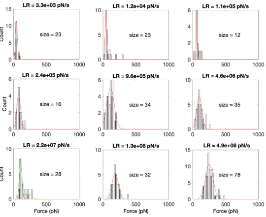
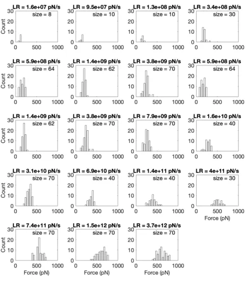
HS-FS Data Processing. Rupture events were detected using semiautomatic home-made routines (MATLAB; MathWorks) from the numerical derivative of the force curves by defining a threshold established by the zero-force baseline noise and depending on the sampling frequency and pulling rate (24). Force curves presenting rupture events were analyzed to measure the rupture forces, rupture lengths, and effective spring constant (Fig. 1B). Loading rates were determined from the slope before rupture (2 to 3 nm) of each force versus time trace. Rupture forces were pooled by loading rate and the corresponding histograms generated (SI Appendix, Figs. S1 and S2). Most probable rupture forces and SDs of rupture forces at each loading rate were calculated from Gaussian fits (SI Appendix, Figs. S1 and S2). When two peaks were clearly distinguishable in the force histograms, distributions were fit-ted using a bimodal function imposing the center of the second peak to be two times that of the first peak. Thus, the first center peak value was used as the average rupture force (SI Appendix, Figs. S1 and S2).
HS-FS Transient Binding. From the list of rupture events, transient or in-termediate binding events were determined from the numerical derivative of the force drop region: from the main rupture event to the zero-force baseline (SI Appendix, Figs. S5 and S6). The numerical derivative of the force drop region was calculated by the five-point stencil method (50). An average filter with a window ranging from 0 to 25 μs was used according to pulling ve-locity and sampling rate. At the lowest velocities, due to the reduced sam-pling rate and the lower rupture forces, shortest events were likely missed. Transient binding events were defined from the time interval between the two most prominent minima within the force drop region including at least one data point of the force derivative with positive value. If this condition was not accomplished or the mean force value for the transient event was within one SD of the zero-force baseline, no rebinding event was consid-ered. The lifetime of the intermediate state was determined from the time interval between these two minima. The force level was determined as the average force of the interval. The distance to the intermediate state (Fig. 3D) was calculated from the force versus extension curves as the distance from the extension at which the main rupture occurs to the average extension of the interval.
HS-FS Viscous Drag Correction. Viscous drag coefficients were calculated for each cantilever type from retraction curves by measuring the drag force exerted on the cantilever at various velocities near the substrate (<200 nm) divided by the retraction velocity (51, 52). The cantilever coefficients on agarose beads were 0.09 pN/(μm·s) and 0.05 pN/(μm·s) for AC10 and AC7 cantilevers, respectively. The viscous drag was corrected by multiplying the viscous drag coefficient by the relative tip velocity. This correction was only significant (∼8% force correction) at the highest velocities achieved with each cantilever type.
MD Simulations. Force probe MD simulations were carried out using the Amber99sb (53) force field together with TIP3P (54) water model and vir-tual interaction sites (55). The electrostatic interaction was calculated with particle-mesh Ewald (56) with a real space cutoff of 1 nm, a grid spacing of 0.12 nm, and cubic interpolation. The same cutoff length was used for the van der Waals interaction. All atom bonds were constraint using LINCS al-gorithm (57). All simulations were performed at a constant number of
particles and a constant temperature coupled to a heat bath at 300 K using the velocity rescaling method (58) and a coupling constant of 0.2 ps. We used the Verlet algorithm (59) with a time step of 4 fs to integrate the equation of motion. In the experimental setup, the cantilever, here de-scribed by a harmonic potential with a spring constant kpull= 100 pN/nm,
was attached to b via a PEG linker. The harmonic potential was moved away from the binding pocket at 12 different velocities, ranging from 0.001 m/s up to 50 m/s. Depending on the applied loading rate the center of the harmonic pulling potential moved up to 12 nm until the simulation was stopped, ensuring that b is completely unbound from SA. In the simulations the linker was described by a WLC potential,
UwlcðxÞ =kBTlc 4lp ! 1−x + xstart lc "−1 −kBTðx + xstartÞ 4lp + kBTðx + xstartÞ2 2lclp ,
with a persistence length lp= 1.4 nm and a contour length lc= 10 nm, similar
to the experimental values (Fig. 1, simulation setup), which was added to GROMACS as a tabulated bonded potential (54). To keep the simulation box size small we shifted the WLC potential by a constant xstart= 7 nm,
never-theless making sure that the forces required to stretch the linker were lower than those to rupture the complex. All simulations were performed at a sodium chloride concentration of 150 mM. The simulation box sizes per-pendicular to the pulling direction were chosen to be 8.5 nm, which is a minimal distance of 0.7 nm between the solute and the periodic boundaries, leading to a minimum distance between SA and its periodic image of more than 1.4 nm. The box length in the pulling direction varied between 18 nm for the faster and 13 nm for the slowest simulations.
The starting structure for the simulations was based on the tetramer PDB ID code 3RY2 (4). In case of the tetramer, only one b was pulled out of the binding pocket to ensure single unbinding events.
Rupture forces and loading rates were determined for each individual force curve. As for experiments, the loading rate was also determined from the slope of the force–time curve before rupture. We calculated the mean and SD of the rupture forces for each loading rate.
Brownian Dynamics Simulations. To extract information on the underlying free-energy landscape along the unbinding reaction coordinate, and in ad-dition to the application of the simple Bell model and more sophisticated theoretical approaches [BSK (15), Friddle-Noy-deYoreo (FNdY) (37), Dudko– Hummer–Szabo (DHS) (14), and CHS (36)], numerical simulations of enforced unbinding with one-dimensional energy landscapes were carried out. To that end, the Smoluchowsky equation,
∂tpðx, tÞ = ∇D ½∇ − βð∇Vðx, tÞÞ$ pðx, tÞ,
was solved numerically for a time-dependent potential Vðx, tÞ = V0ðxÞ − _Fxt, where β = 1=kBT and _F is the applied loading rate. As underlying unbinding
potential, a double-barrier potential V0ðxÞ = 2ΔG1ðxÞ2ð1.5 − yðxÞÞ for x ≤ xβ1
was chosen, with barrier height ΔG1 of the first barrier. The
func-tion yðxÞ =##c1xxβ1+ c2 $ x xβ1+ ω1 $ x
xβ1, with the constants c1= ω1+ ω2− 2 and c2= 3− 2ω1− ω2, served to control the shape of the first barrier,
particu-larly the curvatures ω1and ω2of the well and, respectively, that at the
first barrier top. The above function also serves to control the rupture length xβ1, here defined as the distance between first barrier top and
minimum of the well of the bound state. For xβ1< x < xβ2the potential becomes
Vx>xβ1ðxÞ = V0 %
xβ1&+ 2ðΔG2− ΔG1ÞyðxÞ2ð1.5 − yðxÞÞ
with yðxÞ =x− xβ1
xβ2 and the position of the second barrier xβ2. For all x > xβ2the potential is set to ΔG2, the height of the second barrier.
Trajectories were generated starting from a Boltzmann ensemble p0(x)/
exp(V0(x)) within the well of the bound state. Positions were updated to first
order according to the solution of the Smoluchowski equation for linear potential, xnewdxold−DΔtk BT∇Vðx, tÞ + 1 ffiffiffiffiffiffiffiffiffiffiffiffi 2DΔt p ξðtÞ,
with an integration time step of 0.5 ps, which ensured that less than 5% of the integration steps were larger than 0.05 xβ1. A Gaussian distributed
(vari-ance one) random force ξðtÞ was used. A diffusion constant D = kBT=
γ =4 · 10−11m2=s was found to provide the best fit to the force spectrum.
To reduce computational effort and thus to facilitate the generation of trajectories even for the slowest loading rates, an appropriate biasing potential
Vbiasðx, tÞ = a! x
xβ
"n
+ vðtÞ
was added whenever the (actual) barrier height exceeded 5 kBT, with
a = 1 ncn−1, c =
nv n− 1
and v adapted such that the barrier height of the resulting total potential Vðx, tÞ + Vbiasðx, tÞ remained between 5 and 7 kBT at all times. To compensate for
the reduced barrier height due to the biasing potential and the increased barrier transition probability per integration step, the integration step size was dynam-ically rescaled by an acceleration factor ZbiasðtÞ = Z0ðtÞ, where Z0and Zbiasare the
partition functions of the unperturbed and, respectively, perturbed bound states: Z0ðtÞ = Zxb −∞ expð−βVðx, tÞÞdx and ZbiasðtÞ = Zxb −∞ expð−βðVðx, tÞ + Vbiasðx, tÞÞÞdx.
For each of the loading rates for which experimental or MD simulation derived rupture forces were obtained (Fig. 2), 1,000 trajectories were gen-erated and the resulting individual force at the point of barrier crossing were averaged. The fitting parameters ΔG1, ΔG2, xβ1, xβ2, ω1, and ω2were
varied using simple line-scanning until the χ2(weighted by the SEM) relative
to the 37 experimental/simulation averaged rupture forces was minimal. Uncertainties of the six fitting parameters (given in the caption ofSI Ap-pendix, Fig. S7) were estimated conservatively via nonparametric boot-strapping with 80 replica datasets, each of which was generated by randomly drawing 37 from the 37 rupture forces (allowing for multiple draws of the same data point). Parametric bootstrapping using a Gaussian error model and the SEMs rupture forces yielded slightly smaller uncertainties.
COM Distributions. To calculate the distributions of the COM distance of each MD trajectory, we calculated the distance between the COM of the binding-pocket-forming residues (L25, S27, Y43, S45, V47, G48, A50, W79, R84, A86,
S88, T90, W92, W108, L110, and D128) and the COM of b. This was done starting shortly before rupture and ending when the distance between b and the binding pocket was larger 4 nm.
As we do not see any binding patterns further away than 2 nm we reduced the plotted histograms to a maximal distance of 2 nm. The COM distances were then binned into 200 equally spaced bins and normalized by the total amount of data points.
MD Intermediate States and Transition Plots. To determine the intermediate states, we split the COM distance distributions according to the dominant peaks, such that each peak represents a different intermediate state. We then calculated the transition rates by counting the transitions from state sito
state sjand subtracted the amount of back-transitions (sjto si) for each
combination, resulting in a net transition of−1, 0, or 1. Finally, each rate was averaged for each velocity.
The probabilities for being in an intermediate state were calculated by counting the total time that an intermediate state is visited normalized by the total time spent in all intermediate states. The time spent in the ground state and the unbound state were not taken into account to provide comparability, as the time spent in either of them is arbitrary and depends only on the chosen starting and end point of the rupture event.
Principal Component Analysis of Loop 3–4. To understand the different un-binding pathways, we analyzed the motion of loop 3–4 by performing a principal component analysis on the backbone atoms of residues 44–54. Therefore, a representative simulation was used to calculate the character-istic eigenvectors of the loop 3–4 motion going from a closed conformation (negative values) to an open conformation (positive values). All other simu-lations were projected onto the first eigenvector and analyzed depending on the applied loading rate regime. The time-resolved projections were finally binned along the COM distance and the average projection on the first ei-genvector for each loading rate regime was calculated (SI Appendix, Fig. S10). ACKNOWLEDGMENTS. F.R. and H.G. thank Prof. Klaus Schulten for inspiring discussions, and F.R. and S.S. thank Prof. Toshio Ando for generously providing AC7 cantilevers. This work was supported in part by the Agence National de la Recherche Grants ANR-15-CE11-0007 (BioHSFS) and ANR-11-LABX-0054 (Labex INFORM), European Cooperation in Science & Technology Action TD1002-10006, and Deutsche Forschungsgemeinschaft Grant SFB 755.A5.
1. Koshland DE (1958) Application of a theory of enzyme specificity to protein synthesis. Proc Natl Acad Sci USA 44:98–104.
2. Fischer E (1894) Einfluss der configuration auf die wirkung der enzyme. Ber Dtsch Chem Ges 27:2985–2993.
3. Frederick KK, Marlow MS, Valentine KG, Wand AJ (2007) Conformational entropy in molecular recognition by proteins. Nature 448:325–329.
4. Le Trong I, et al. (2011) Streptavidin and its biotin complex at atomic resolution. Acta Crystallogr D Biol Crystallogr 67:813–821.
5. Chilkoti A, Stayton PS (1995) Molecular-origins of the slow streptavidin-biotin disso-ciation kinetics. J Am Chem Soc 117:10622–10628.
6. Laitinen OH, Hytönen VP, Nordlund HR, Kulomaa MS (2006) Genetically engineered avidins and streptavidins. Cell Mol Life Sci 63:2992–3017.
7. Hyre DE, et al. (2006) Cooperative hydrogen bond interactions in the streptavidin-biotin system. Protein Sci 15:459–467.
8. Koussa MA, Halvorsen K, Ward A, Wong WP (2015) DNA nanoswitches: A quantitative platform for gel-based biomolecular interaction analysis. Nat Methods 12:123–126. 9. Chivers CE, et al. (2010) A streptavidin variant with slower biotin dissociation and
increased mechanostability. Nat Methods 7:391–393.
10. Merkel R, Nassoy P, Leung A, Ritchie K, Evans E (1999) Energy landscapes of receptor-ligand bonds explored with dynamic force spectroscopy. Nature 397:50–53. 11. Florin EL, Moy VT, Gaub HE (1994) Adhesion forces between individual
ligand-receptor pairs. Science 264:415–417.
12. Lee GU, Kidwell DA, Colton RJ (1994) Sensing discrete streptavidin biotin interactions with atomic-force microscopy. Langmuir 10:354–357.
13. Evans E, Ritchie K (1997) Dynamic strength of molecular adhesion bonds. Biophys J 72: 1541–1555.
14. Dudko OK, Hummer G, Szabo A (2006) Intrinsic rates and activation free energies from single-molecule pulling experiments. Phys Rev Lett 96:108101.
15. Bullerjahn JT, Sturm S, Kroy K (2014) Theory of rapid force spectroscopy. Nat Commun 5:4463.
16. Teulon J-M, et al. (2011) Single and multiple bonds in (strept)avidin-biotin interac-tions. J Mol Recognit 24:490–502.
17. Moy VT, Florin EL, Gaub HE (1994) Intermolecular forces and energies between li-gands and receptors. Science 266:257–259.
18. Sedlak SM, et al. (2017) Monodisperse measurement of the biotstreptavidin in-teraction strength in a well-defined pulling geometry. PLoS One 12:e0188722. 19. Rico F, Moy VT (2007) Energy landscape roughness of the streptavidbiotin
in-teraction. J Mol Recognit 20:495–501.
20. Jeney S, Mor F, Koszali R, Forró L, Moy VT (2010) Monitoring ligand-receptor inter-actions by photonic force microscopy. Nanotechnology 21:255102.
21. Pincet F, Husson J (2005) The solution to the streptavidin-biotin paradox: The influ-ence of history on the strength of single molecular bonds. Biophys J 89:4374–4381. 22. Neupane K, et al. (2016) Direct observation of transition paths during the folding of
proteins and nucleic acids. Science 352:239–242.
23. Yu H, Siewny MGW, Edwards DT, Sanders AW, Perkins TT (2017) Hidden dynamics in the unfolding of individual bacteriorhodopsin proteins. Science 355:945–950. 24. Rico F, Gonzalez L, Casuso I, Puig-Vidal M, Scheuring S (2013) High-speed force
spectroscopy unfolds titin at the velocity of molecular dynamics simulations. Science 342:741–743.
25. Takahashi H, Rico F, Chipot C, Scheuring S (2018) α-Helix unwinding as force buffer in spectrins. ACS Nano 12:2719–2727.
26. Grubmüller H, Heymann B, Tavan P (1996) Ligand binding: Molecular mechanics calculation of the streptavidin-biotin rupture force. Science 271:997–999. 27. Izrailev S, Stepaniants S, Balsera M, Oono Y, Schulten K (1997) Molecular dynamics
study of unbinding of the avidin-biotin complex. Biophys J 72:1568–1581. 28. Walton EB, Lee S, Van Vliet KJ (2008) Extending Bell’s model: How force transducer
stiffness alters measured unbinding forces and kinetics of molecular complexes. Biophys J 94:2621–2630.
29. Yuan C, Chen A, Kolb P, Moy VT (2000) Energy landscape of streptavidin-biotin complexes measured by atomic force microscopy. Biochemistry 39:10219–10223. 30. Abraham MJ, et al. (2015) GROMACS: High performance molecular simulations
through multi-level parallelism from laptops to supercomputers. SoftwareX 1:19–25. 31. Kutzner C, et al. (2015) Best bang for your buck: GPU nodes for GROMACS
bio-molecular simulations. J Comput Chem 36:1990–2008.
32. Hinterdorfer P, Baumgartner W, Gruber HJ, Schilcher K, Schindler H (1996) Detection and localization of individual antibody-antigen recognition events by atomic force microscopy. Proc Natl Acad Sci USA 93:3477–3481.
33. Heymann B, Grubmüller H (2000) Dynamic force spectroscopy of molecular adhesion bonds. Phys Rev Lett 84:6126–6129.
34. Hummer G, Szabo A (2003) Kinetics from nonequilibrium single-molecule pulling experiments. Biophys J 85:5–15.
35. Makarov DE (2014) Communication: Does force spectroscopy of biomolecules probe their intrinsic dynamic properties? J Chem Phys 141:241103.
36. Cossio P, Hummer G, Szabo A (2016) Kinetic ductility and force-spike resistance of proteins from single-molecule force spectroscopy. Biophys J 111:832–840.
Rico et al. PNAS Latest Articles | 7 of 8
BIOPHYSICS
AND
COMPUTATION
AL
37. Friddle RW, Noy A, De Yoreo JJ (2012) Interpreting the widespread nonlinear force spectra of intermolecular bonds. Proc Natl Acad Sci USA 109:13573–13578. 38. Dudko OK (2016) Decoding the mechanical fingerprints of biomolecules. Q Rev
Biophys 49:e3.
39. Lu H, Schulten K (2000) The key event in force-induced unfolding of Titin’s immu-noglobulin domains. Biophys J 79:51–65.
40. Gräter F, Shen J, Jiang H, Gautel M, Grubmüller H (2005) Mechanically induced titin kinase activation studied by force-probe molecular dynamics simulations. Biophys J 88:790–804.
41. Wolynes PG (1997) Folding funnels and energy landscapes of larger proteins within the capillarity approximation. Proc Natl Acad Sci USA 94:6170–6175.
42. Voß B, Seifert R, Kaupp UB, Grubmüller H (2016) A quantitative model for camp binding to the binding domain of mlok1. Biophys J 111:1668–1678.
43. Wang J, Verkhivker GM (2003) Energy landscape theory, funnels, specificity, and optimal criterion of biomolecular binding. Phys Rev Lett 90:188101.
44. Hohsaka T, et al. (2004) Position-specific incorporation of dansylated non-natural amino acids into streptavidin by using a four-base codon. FEBS Lett 560:173–177.
45. Murakami H, Hohsaka T, Ashizuka Y, Hashimoto K, Sisido M (2000) Site-directed in-corporation of fluorescent nonnatural amino acids into streptavidin for highly sen-sitive detection of biotin. Biomacromolecules 1:118–125.
46. Sader JE, et al. (2016) A virtual instrument to standardise the calibration of atomic force microscope cantilevers. Rev Sci Instrum 87:093711.
47. Sumbul F, Marchesi A, Takahashi H, Scheuring S, Rico F (2018) High-speed force spectroscopy for single protein unfolding. Nanoscale Imaging: Methods and Protocols, ed Lyubchenko YL (Springer, New York), pp 243–264.
48. Tees DFJ, Waugh RE, Hammer DA (2001) A microcantilever device to assess the effect of force on the lifetime of selectin-carbohydrate bonds. Biophys J 80:668–682. 49. Johnson KC, Thomas WE (2018) How do we know when single-molecule force
spec-troscopy really tests single bonds? Biophys J 114:2032–2039. 50. Sauer T (2011) Numerical Analysis (Pearson, Essex, UK).
51. Janovjak H, Struckmeier J, Müller DJ (2005) Hydrodynamic effects in fast AFM single-molecule force measurements. Eur Biophys J 34:91–96.
52. Alcaraz J, et al. (2002) Correction of microrheological measurements of soft samples with atomic force microscopy for the hydrodynamic drag on the cantilever. Langmuir 18:716–721.
53. Hornak V, et al. (2006) Comparison of multiple Amber force fields and development of improved protein backbone parameters. Proteins 65:712–725.
54. Jorgensen WL, Chandrasekhar J, Madura JD, Impey RW, Klein ML (1983) Comparison of simple potential functions for simulating liquid water. J Chem Phys 79:926–935. 55. Feenstra KA, Hess B, Berendsen HJC (1999) Improving efficiency of large time-scale
molecular dynamics simulations of hydrogen-rich systems. J Comput Chem 20: 786–798.
56. Darden T, York D, Pedersen L (1993) Particle mesh Ewald: An N·log(N) method for Ewald sums in large systems. J Chem Phys 98:10089–10092.
57. Hess B, Bekker H, Berendsen HJC, Fraaije JGEM (1997) LINCS: A linear constraint solver for molecular simulations. J Comput Chem 18:1463–1472.
58. Bussi G, Donadio D, Parrinello M (2007) Canonical sampling through velocity rescal-ing. J Chem Phys 126:014101.
59. Verlet L (1967) Computer “experiments” on classical fluids. I. Thermodynamical prop-erties of Lennard-Jones molecules. Phys Rev 159:98–103.
1
Supplementary Information for
Heterogeneous and rate-dependent streptavidin-biotin unbinding
revealed by high-speed force spectroscopy and atomistic simulations
Felix Rico
1‡*, Andreas Russek
2‡, Laura González
3, Helmut Grubmüller
2*, and Simon Scheuring
4,5* 1Aix Marseille Univ, CNRS, INSERM, LAI, Marseille, France
2
Department of Theoretical and Computational Biophysics, Am Faßberg 11, Göttingen, Germany
3Department of Electronics, Universitat de Barcelona, c/ Marti Franques 1, 08028 Barcelona,
Spain
4
Department of Anesthesiology, Weill Cornell Medical College, 1300 York Ave, New York, NY
10065, USA
5
Departments of Physiology and Biophysics, Weill Cornell Medical College, 1300 York Ave,
New York, NY 10065, USA
*