Control of mobile networks using dynamic vehicle routing

Control of Mobile Networks Using Dynamic

Vehicle Routing

by

Holly A. Waisanen-Hatipoglu

B.S. Applied Mathematics

M.S. Systems and Control Engineering

Case Western Reserve University, 2003

Submitted to the Department of Electrical Engineering and Computer

Science

in partial fulfillment of the requirements for the degree of

Doctor of Philosophy

at the

MASSACHUSETTS INSTITUTE OF TECHNOLOGY

September 2007

©

Massachusetts Institute of Technology 2007. All rights reserved.

i i a .

Author....

..

....

.

...

...

...

.

Department of Electrical Engineering and Computer Science

August 14, 2007

Certified by.

Munther A. Dahleh

Professor of Electrical Engineering

Thesis Supervisor

Certified by...

... t . .... .. ..

Devavrat Shah

Pr

r f lectrical Engineering

-I,

~siso-1fr-vior

Accepted by...

Professor Arfi'r C. Smith

Chair, Department Committee on Graduate Students

ARCHIVES

OCT t

2 207

Control of Mobile Networks Using Dynamic Vehicle Routing

by

Holly A. Waisanen-Hatipoglu

Submitted to the Department of Electrical Engineering and Computer Science

on August 14, 2007, in partial fulfillment of the

requirements for the degree of

Doctor of Philosophy

Abstract

This thesis considers the Dynamic Pickup and Delivery Problem (DPDP), a dynamic

multi-stage vehicle routing problem in which each demand requires two spatially

separated services: pickup service at its source location and then delivery service

at its destination location. The Dynamic Pickup and Delivery Problem arises in

many practical applications, including taxi and courier services, manufacturing and

inventory routing, emergency services, mobile sensor networks, Unmanned Aerial

Vehicle (UAV) routing, and delay tolerant wireless networks.

The main contribution of this thesis is the quantification of the delay performance of

the Dynamic Pickup and Delivery Problem as a function of the number of vehicles,

the total arrival rate of messages, the required message service times, the vehicle

velocity, and the network area. Two lower bounds are derived. First, the Universal

Lower Bound quantifies the impact of spatially separated service locations and system

loading on average delay. The second lower bound is derived by reducing the

two-stage Dynamic Pickup and Delivery Problem to the single-two-stage Dynamic Traveling

Repairperson Problem (DTRP). Policies are then presented for which these lower

bounds are tight as a function of the system scaling parameters (up to a constant).

The impact of information and inter-vehicle relays is also studied.

The last part of this thesis examines the application of the Dynamic Pickup and

Delivery Problem to mobile multi-agent wireless networks from a physical layer

per-spective, seeking insights for the control of the network to achieve trade-offs between

throughput and delay.

Thesis Supervisor: Munther A. Dahleh

Title: Professor of Electrical Engineering

Thesis Supervisor: Devavrat Shah

Acknowledgments

My doctoral experience has been less about research and more about living my life.

I have many to thank for taking me this far.

First, I thank my two advisors, Professors Munther Dahleh and Devavrat Shah. Their

advising styles and research interests have been complementary, and I could not have

progressed without them both. They are both genuinely kind people, and it has been

a pleasure to know them. I thank my committee as a whole for making it possible for

me to finish on time and for supporting my career interests, though they lie outside

of academic research for now.

Thanks also go to

" Professor Alexandre Megretski for setting a high academic standard.

" Professor Eytan Modiano for making my TA experience as fruitful as possible.

* Georgios Kotsalis and Erin Aylward for their enthusiasm for research.

" Other officemates and friends in the department: Keith Santarelli, Sleiman

Itani, Giola Katsargyri, Mike Rinehart, Hoho, Sridevi Sarma, Danielle Tarraf,

and Nuno Martins.

" My friends from first and second year: Zach Thomas, Shubham Mukherjee,

Vasanth Sarathy, Akshay Naheta, Keith Herring, and Alex Tsankov.

" Kishori Deshpande, my roommate and friend.

" Everyone I met in GW6, Graduate Student Council, and at Edgerton House.

Many thanks go to Laura Zager for providing me a friendly ear these last four years.

I value our friendship very much. I wish I could be around next year to support you

as you have supported me, but I'll only be a phone call or plane ride away.

Last but not least, for so many reasons, I would not be where I am today without

the loving support and sacrifice of Cem Hatipoglu. Seni gok seviyorum.

Contents

1 Introduction 15

1.1 Literature Review . . . . 16

1.1.1 Dynamic Vehicle Routing . . . . 17

1.1.2 Other Mobile Networks . . . . 21

1.1.3 Throughput and Delay in Wireless Networks . . . . 21

1.2 R esults . . . . 23

1.2.1 Universal Lower Bounds for Dynamic Pickup and Delivery . . 24

1.2.2 Dynamic Pickup and Delivery with No Relays . . . . 24

1.2.3 Dynamic Pickup and Delivery with Relays . . . . 25

1.2.4 Throughput-Delay Tradeoff in Wireless Networks with Con-trolled Mobility . . . . 26 1.3 Organization of Thesis . . . . 26 2 Problem Formulation 27 2.1 M odel . . . . 27 2.2 Control Policies . . . . 29 2.2.1 Assignment Policies . . . . 29 2.2.2 Service Policies . . . . 32 2.3 Performance Metrics . . . . 33 2.3.1 Preliminary Definitions . . . . 34 2.3.2 Average Delay . . . . 35

2.3.4 Number in System . . . . 41

2.3.5 System Utilization and Stability . . . . 42

2.4 Problem Statement . . . . 43

3 Preliminary Technical Details 45 3.1 General Probability ... 45

3.1.1 Jensen's Inequality ... ... 45

3.1.2 Implications of Positive Correlation . . . . 45

3.1.3 Geometric Probability . . . . 46

3.2 Queueing Theory . . . . 46

3.2.1 Queueing Notation . . . . 46

3.2.2 Stability of GI/G/1 Queues and Queuing Networks . . . . 47

3.2.3 Upper Bound on Waiting Time in GI/G/1 Queue . . . . 47

3.2.4 Little's Law . . . . 48

3.2.5 Arrival and Departure Distributions . . . . 49

3.3 Euclidean TSP Tour Length . . . . 49

3.3.1 Asymptotic Performance . . . . 49

3.3.2 Worst-Case Performance . . . . 50

3.4 Dynamic Traveling Repairperson Problem . . . . 51

4 Universal Lower Bounds 53 4.1 Universal Lower Bound for Poisson Arrivals . . . . 54

4.1.1 Preliminary Lower Bound for Single Vehicle . . . . 54

4.1.2 Universal Lower Bound for Multi-Vehicle . . . . 56

4.2 Universal Lower Bound for Batching Policies . . . . 58

4.2.1 Batching Policies Preliminaries . . . . 59

4.2.2 Preliminary Lower Bound for Single Vehicle . . . . 60

4.2.3 Universal Lower Bound for Multi-Vehicle, Batching Policies. . 64 4.2.4 Universal Lower Bound Corollary for Batching Policies . . . . 65

5 No Relay DPDP

5.1 Lower Bounds on Average Delay ...

5.1.1 A Relaxation of OPT ...

5.1.2 Lower Bound: Source Only ...

5.1.3 Lower Bound: Source and Destination

5.2 Policies . . . . 5.2.1 Source Only Policy ...

5.2.2 Source and Destination Policy . . . . .

5.3 Conclusions . . . .

6 Single Relay DPDP

6.1 Lower Bound on Average Delay . . . .

6.2 Upper Bounds for Single-Relay Policies . . . .

6.2.1 Synchronous Single-Relay Policy . . . .

6.2.2 Other Relay Policies - The 1-Depot Policy .

6.3 Conclusions . . . .

6.3.1 Optimality of Single Relay . . . .

7 Wireless DPDP

7.1 Model and Problem Statement . . . .

7.1.1 Nodes, Messages, and Vehicles . . . .

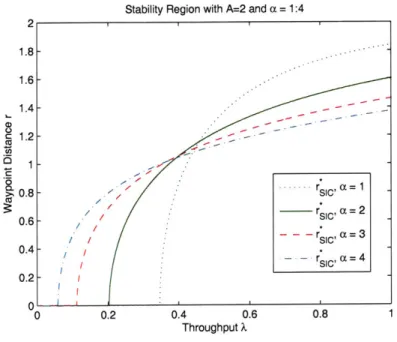
7.1.2 Wireless Model . . . . 7.1.3 Control Policies . . . . 7.1.4 Performance Measures . . . . 7.1.5 Problem Statement . . . . 7.1.6 Organization . . . . 7.2 Stability Analysis . . . .

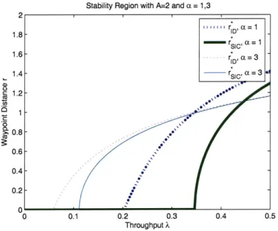
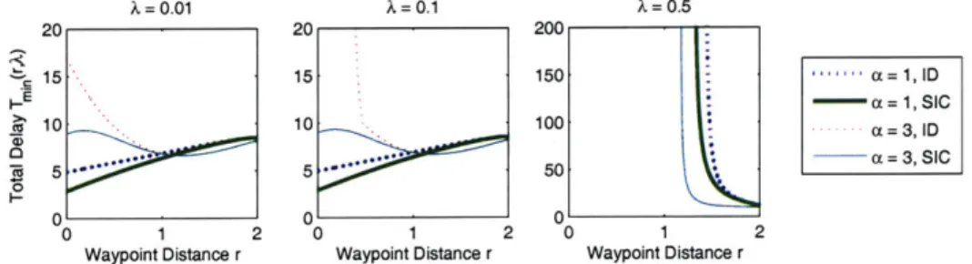
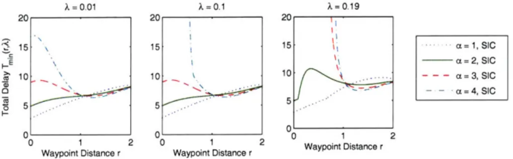
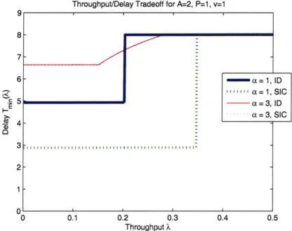
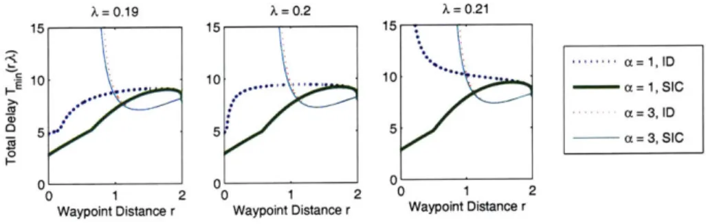
7.3 Optimal Batch Scaling and Delay for fixed r and A

7.3.1 Analytical Characterization of Tmin (r, A) 7.3.2 Graphical Characterization of Tmin(r, A) 7.4 Optimal Throughput/Delay Tradeoff . . . .

89

90

90 90 95

96

97 99 . . . . 100 . . . . 100 . . . . 101 . . . . 103 . . . . 104 . . . . 104 . . . . 105 . . . . 105 . . . . 108 . . . . 109 . . . . 111 .. .... 112 69

. . . .

70

. . . . 71 . . . . 72 . . . . 75 . . . . 79 . . . . 79 . . . . 85 . . . . 88

7.5 Conclusions . . . .1

8 Discussion 117 8.1 Scaling Interpretation of Results . . . . 117

8.2 Significance of Policy Restrictions . . . . 119

8.3 Extensions of Methods . . . . 121

8.4 Future Work in Wireless . . . . 121

8.5 Conclusion . . . . 122

A Extended proof of DTRP 123 B Proof of Little's Law for the onsite system 131 C Proof of batch queuing time 137 . . . . . 114

List of Figures

7-1 Stability Region for test case . . . . 107

7-2 Stability Region for test case - a = 1,2,3,4 . . . . 108

7-3 Delay as a function of r with optimal batch size . . . . 111

7-4 Delay as a function of r with optimal batch size, a = 1, 2,3,4 . . . . . 112

7-5 Optimal Delay as a function of A, Comparison . . . . 113

List of Tables

7.1 Detailed Rate Profiles for Decoding Schemes . . . 102

Chapter 1

Introduction

Mobile networks are characterized by a set of servers that travel throughout a given region to collectively perform a set of tasks. The motion and service activity of the mobile servers is to be controlled to optimize some performance measure based on the completion of tasks and consumption of server resources. Several varieties of tasks may be defined, including surveillance coverage of the region, convergence to a fixed vehicle formation, and service of a series of externally generated demands. This thesis focuses on the latter type of mobile network as an instance of a Dynamic Vehicle Routing Problem.

Vehicle Routing Problems (VRPs) constitute a class of well-studied problems in the Operations Research and Applied Mathematics literature. The classical example of a VRP is the Traveling Salesperson Problem (TSP) in which a single server is to visit each member of a fixed set of locations such that the total travel cost is minimized. Each location may be viewed as a demand which is served when the server passes through that location. Many vehicle routing problems may be viewed as extensions of this classical static and deterministic VRP. Several extensions may be envisioned, including more complex types of demand service, dynamic arrival of demands, and the use of multiple servers.

dynamic multi-stage VRP in which each demand requires service at each of several spatially separated locations, specifically pickup service at its source location and then delivery service at its destination location elsewhere in region. The DPDP prob-lem arises in many practical applications. For example, consider a scenario where people are demands who telephone a cab-service exchange to request a ride. The cab-service exchange is to decide which cab picks up (and delivers) each person and at what time, such that each customer is completely served with minimum average de-lay. This problem is also known as Dial-a-Ride problem (DARP). Other applications include courier services, manufacturing and inventory routing, less-than-truckload (LTL) trucking, emergency services, mobile sensor networks, and Unmanned Aerial Vehicle (UAV) routing. Surveys [13] and [25] contain references to several of these applications.

Of particular interest to this thesis is the quantification of the performance of the

network as a function of several scaling parameters, including the number of vehicles, the total arrival rate of messages, the required service times, and to a lesser extent, the vehicle velocity and network area. Such analysis exists for a single-stage problem known as the Dynamic Traveling Repairperson Problem. Our results for the two-stage DPDP and the four-stage DPDP (with Relays) are the first of their kind. Besides analyzing system performance as a function of the scaling parameters, we also examine the impact of several other system qualities, including information structure and service type. Our results provide general methods which are different than those in the existing literature.

1.1

Literature Review

We first review the previous research on dynamic vehicle routing problems, including the DPDP, in the context of operations research. We then address existing research on other types of mobile networks, including pickup and delivery networks in which services may be performed remotely via wireless transmission.

1.1.1

Dynamic Vehicle Routing

The relevant research in dynamic vehicle routing may be grouped into three areas

that address specific aspects of the Dynamic Pickup and Delivery Problem as an

extension of the canonical vehicle routing problem, the Traveling Salesperson Problem

(TSP). After reviewing previous research on the TSP, we first consider the impact of

demand uncertainty in dynamic and stochastic problems. Next, we look at methods

for incorporating multiple vehicles via a demand assignment component. Finally, we

examine the impact of multi-stage demand service.

The Traveling Salesperson Problem (TSP)

In the classical static and deterministic vehicle routing problem, a fixed set of demands is specified a priori and the solution is a route through these demands that minimizes

some collective cost of service, usually expected total travel time. The most

well-studied static and deterministic vehicle routing problem is the Traveling Salesperson

Problem, in which a salesman must determine the shortest route through a fixed set of cities in his territory. Classically, the TSP is formulated on an undirected graph with distances between cities denoted by edge weights between nodes. The TSP is known to be NP-complete. Various heuristics have been developed to find approximately optimal polynomial-time solutions to the TSP [19, 31) and its natural counterpart,

the directed TSP

[291.

In the Euclidean TSP, cities are taken to be points arbitrarily distributed in R2

with distances corresponding to the Euclidean distance measure. In the case that there are N cities uniformly distributed in a region of area A , the expected length of the TSP tour scales as LN ;

%/T4v/.N

when N -+ oo. This asymptotic result is originally due to Beardwood, Halton, and Hammersley [3], but has been more recently studied in [17). This theorem will be important to our analysis and will be stated precisely in Section 3.3. Heuristics for computing approximately optimal polynomial-time solutions to the Euclidean TSP are presented in [2].

Static to Dynamic

In a static and deterministic VRP, the set of demands is fixed a priori, and the vehicle control consists of computing a single route through these demands to optimize a given cost function. In a dynamic and stochastic VRP, new demands arrive according to a stochastic process over time, and the solution is a control policy that that determines how the vehicles' routes evolve as a function of the demands in the system. A common objective is to minimize the average message time in system over an infinite time horizon rather than completion time of the fixed set.

Dynamic vehicle routing problems have received much less attention than their static counterparts. Recent surveys on dynamic vehicle routing problems include [13, 24].

Common solution methods for the dynamic problem include the reduction of the dynamic problem to a series of static problems via periodic reoptimization or batching.

From a theoretical standpoint, the most significant analysis of dynamic vehicle routing problems is the the work on the single-stage Dynamic Traveling Repairperson Problem (DTRP) by Bertsimas and van Ryzin [4, 5, 6]. These papers obtain several policies which achieve order-optimal average delay for the problem.

Intuitively, the DPDP seems similar to the DTRP as both the pickup and delivery of messages in the DPDP could be treated as separate requests in the DTRP problem setup. This thesis shows that this is indeed the case when messages may be relayed between vehicles. However, when we include the restriction that the vehicle that picks up a message must also deliver it, the pickup and delivery services of a single mes-sage are strongly linked, making our problem significantly distinct from the DTRP. As we shall see, the optimal solutions to these problems are both qualitatively and quantitatively different.

Single-vehicle to Multi-vehicle

When there are multiple vehicles to perform the system services, the optimal solution

becomes more complex as not only service order but also service assignments to the

vehicles must be determined.

Typical assignment methods for the static single-stage problem rely on the intuition

that demands that are located close together ought to be served by the same

vehi-cle. Two popular algorithms incorporate this intuition via a two-step process. In

partitioning algorithms, an optimal TSP tour is found through all of the demands

and then the tour is partitioned such that each vehicle travels the TSP route through

a subset of the demands and the total vehicle travel cost is minimized. Clustering

algorithms take the reverse approach, first assigning each vehicle to a subset of points

and then leaving each vehicle to determine the TSP tour through just its own subset

[25].

This intuition does not extend to the Pickup and Delivery Problem when the vehicle

that picks up a message must also deliver it. Even if source locations are

geograph-ically close, destination locations may be spread throughout the region. Balancing

the clustering of source locations and destination locations served by a single vehicle

in a multi-vehicle setup will be an important intuitive insight in our work on the

multi-vehicle DPDP.

Repair to Pickup and Delivery

Recent survey papers on Pickup and Delivery Problems (PDPs), both static and dynamic, include [9, 25]. We briefly summarize some of these results below.

The static single-vehicle pickup and delivery problem expands upon the TSP to in-clude a delivery requirement. Not only does this delivery requirement double the number of locations to be visited, but it also imposes a precedence constraint on the order in which the locations may be visited. In the case that the objective is to

minimize the completion time of a fixed set of demands, this may be formulated as a directed TSP. A straightforward dynamic program may also be used to solve for the optimal solution associated with other cost functions. Other solution methods include branch and bound algorithms that incorporate the precedence constraints. Approximations to the static PDP include clustering and routing algorithms similar to those for the TSP, although the analysis is much more complex for the two-stage problem (see [25]).

A problem similar to the Dynamic Pickup and Delivery Problem has been studied as

the Online Dial-a-Ride Problem (OLDARP). In this problem, like the DTRP problem, demands arrive according to a Poisson process of time intensity A. The messages need to be picked up by vehicles from a random arrival location and dropped off at random destination location. This problem has been studied by [10, 21]. Vehicles are usually assumed to have unit or finite capacity, that is, each vehicle can transport only one or finitely many messages at a time. The goal of the OLDARP problem is usually to minimize the service completion time of a collection of messages arriving during a finite time interval. Recent analysis in this problem has focused on competitive analysis to compare the performance of periodic reoptimization methods with static

and deterministic solutions subject to time constraints.

The single-vehicle Dynamic Pick-up and Delivery Problem (DPDP) was analyzed in

[32]. In this setup, a single service vehicle is responsible for picking up and delivering

all messages that arrive. The goal is to minimize the average delay experienced by all messages. Analysis is performed for vehicles with both finite and infinite capacity, and several policies are analyzed in both the heavily and lightly loaded cases, using methods similar to those for the DTRP. In our work, we develop novel proof methods to study the multi-vehicle Dynamic Pickup and Delivery Problem.

1.1.2

Other Mobile Networks

The single-stage, multi-vehicle dynamic vehicle routing problem (i.e. the DTRP)

has received attention in the controls community of late, motivated by applications

to Unmanned Aerial Vehicles (UAVs) and other mobile sensing networks. A

decen-tralized method for computing locally optimal solutions to the m-vehicle DTRP was

presented in [11]. This work applied previous research on decentralized algorithms

for the optimal placement of sensors to provide full coverage of a region with event

locations represented by a continuous distribution [7]. The optimal sensor placement

problem is closely related to the m-median problem and the optimal idle positioning

of the vehicles in a lightly-loaded DTRP system. Other work has considered the

im-pact of vehicle constraints, such as finite turning radius, on the solution of the static

and deterministic Repairperson Problem [26, 27].

In general, there are several possible extensions of the classical dynamic vehicle

rout-ing problem, the Dynamic Travelrout-ing Repairperson Problem. Likewise, the Dynamic

Pickup and Delivery Problem may be viewed as a two-stage extension of the

single-stage DTRP.

1.1.3

Throughput and Delay in Wireless Networks

For many wireless network applications, including video and voice transmission, the

goal is to provide a point-to-point path between each pair of nodes in the network

such that any message that arises may be routed immediately to its destination. In

contrast, in delay-tolerant networks, such a point-to-point path need not exist at each

time instant, but the nodes may store the messages and forward them to the required

connections over time as they move closer to other nodes in the network.

The main application we consider is a delay-tolerant communication network in which

messages orginating in a geographic region must be delivered to their destinations

elsewhere in the region. This service is carried out by a number of mobile nodes or

vehicles. This differs from usual vehicle routing problems in that each node is capable of transmitting messages wirelessly to the vehicle and to other nodes.

A distinct characteristic of wireless transmission is interference: a wireless

transmis-sion by one node may adversely affect other transmistransmis-sions occuring simultaneously. Interference generally implies that to allow the greatest number of nodes to transmit simultaneously, wireless transmissions should only take place over short distances to avoid creating interference over large regions. Since messages may be destined to loca-tions far from their origin, several wireless transmissions may be required for delivery unless there is another method of transport. If the nodes are mobile, messages may also be physically carried over distances in the region. Physical transport of messages has the advantage that it does not create interference and many messages may be carried at one time by a single node. However, node velocity is typically much less than the speed of electromagnetic propagation of wireless transmissions. Therefore, physical transport is a much slower method of delivering messages.

Two important performance measures characterizing wireless networks are through-put and delay. Delay is defined, as in the DPDP, to be the time from message arrival to delivery. Throughput is defined to be the average number of bits to be delivered to their destinations each time unit.

Several previous works have considered varying the amounts of wireless transmission and physical transport of messages in communication networks to study the effect of these methods of message delivery on the throughput and delay characteristics of the network. Gupta and Kumar [16] introduced a random network model to study throughput scaling of fixed wireless networks in which nodes are not mobile and thus messages are delivered solely by wireless transmission. They showed that, under the random network model, the maximal achievable throughput per node, T(n) scales as

E(1/V/nlogin)

for a network of n nodes (see Section 2.1 for a definition of order notation). That is, as the number of nodes and the traffic they bring to the network increases, the throughput achievable by each node goes to 0. Subsequently, Gross-glauser and Tse [15] showed that by using node mobility, it is possible to achieve

optimal per node throughput scaling, T(n) =

E(1).

That is, by using physical trans-port to carry messages without creating wireless interference, the throughput per node remains constant regardless of the number of nodes.

These results, however did not address the issue of delay performance. El Gamal, Mammen, Prabhakar and Shah [12] posed the question of achievable throughput and delay tradeoff. They obtained the following optimal tradeoff: (a) for fixed random networks, the throughput per node, T(n) and delay per packet, D(n) are related as

T(n) =

e(D(n)/n) for T(n)

= O(1/v/nlogn); and (b) for mobile networks with each node performing independent random walk, for most of the throughput, the delay scales D(n) =

e(n

log n). The result of [12] for mobile networks provides a pessimistic conclusion: even at the loss of significant throughput, the delay can not be reduced under a random walk based mobility model.

In search of better delay scaling, various authors [20, 22, 33] have suggested different mobility models. While some of these models provide significant delay reduction at the loss of throughput, they are far from being realistic. Many ignore the physical constraint on the velocity of node. Most assume that node motion is completely random, regardless of the current message delivery requirements. In summary, most of the previous results assume a certain mobility model in order to study delay and throughput of network. Because they consider specific models, they are not able to

make statements on optimal performance achievable under any mobility model. The work of [28] has recently analyzed the minimum worst case delay in a delay-tolerant network with controlled mobility. Other than that paper, little attention has been given to the throughput/delay tradeoff problem with controlled mobility.

1.2

Results

The contributions of this thesis are divided into four main chapters. The first main chapter provides a general lower bound on the delay performance of any Pickup and

Delivery problem. The next two chapters are divided according to whether messages can be relayed between vehicles. The no relay problem is more closely related to classical vehicle routing as described above. Finally, the fourth main chapter contains some preliminary work on the mobile wireless network problem.

The optimality of our results is stated in terms of order optimality, that is, optimal scaling of performance as a function of the system parameters, such as arrival rate, number of vehicles, and the area of the region. We do not seek the optimal solution for a specific realization of the stochastic network. The nontriviality of the order optimal bounds we derive reveals the complexity of finding complete optimal solutions.

1.2.1

Universal Lower Bounds for Dynamic Pickup and

De-livery

In the Dynamic Pickup and Delivery Problem, vehicles must pause at a service loca-tion for the duraloca-tion of the message pickup and delivery service times. This implies that while vehicles are traveling, they are not performing work, in the sense of directly servicing a single message. This restriction implies a lower bound on message delay which we will call a Universal Lower Bound. This lower bound makes an impor-tant connection between dynamic vehicle routing problems and non-work-conserving queueing systems. This bound may also be generalized for analysis of other multi-stage systems.

1.2.2

Dynamic Pickup and Delivery with No Relays

The Dynamic Pickup and Delivery Problem with No Relays refers to the case in which the vehicle that picks up a message must be the one to deliver it. The goal is to find bounds on the minimum average message delay achievable by any valid control policy for the DPDP.

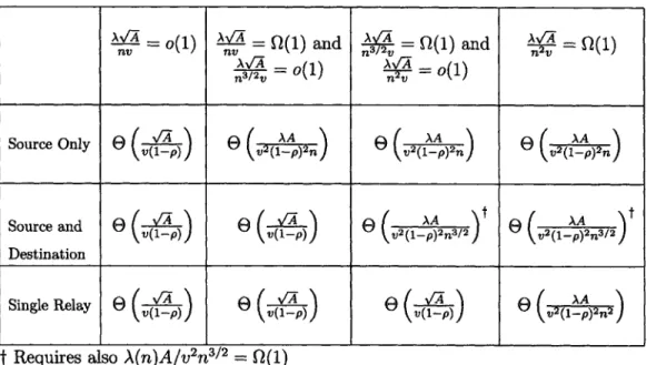
place for making the control decisions. In the Source Only structure, only message source locations are known before the message is picked up. In the Source and Des-tination structure, both the source and desDes-tination locations of messages are known as soon as the message arrives. We will prove lower bounds on the average message delays achieveable by control policies from these two groups. We will further propose policies that adhere to these information structures and will show that the order of the asymptotic delay scaling demonstrated by these policies matches that of the lower bounds for all scaling ranges of the arrival rate A as a function of n. Therefore these policies are order optimal and the lower bounds may be achieved.

The lower bound results are achieved by formulating the multi-vehicle control policies as a collection of joint source and destination densities that capture the assignment policy for each of the vehicles. Existing results in the single-stage Dynamic Traveling Repairperson Problem (DTRP) and joint constraints on the probability densities of valid control policies form an optimization problem which may then be used to lower bound the delay for any control policy. The effects of the information are reflected in the joint constraints. Upper bounds are computed by computing the average delay for specific batching policies which are found to be order optimal. From a system design standpoint, these scalings quantify the perfomance improvements achievable by adding additional information gathering capabilities to the vehicles.

1.2.3

Dynamic Pickup and Delivery with Relays

As long as vehicles are required to perform physical pickups and deliveries at the source and destination locations, the DTRP lower bound serves as a lower bound on the DPDP problem. We show that this lower bound can be achieved by removing the restriction that the same vehicle that picks up a message is the one that delivers it. In fact, we show that this order optimal delay may be achieved with each message being relayed only once, and therefore additional relays cannot improve performance.

1.2.4 Throughput-Delay Tradeoff in Wireless Networks with

Controlled Mobility

Previous analysis in throughput scaling as a function of n, the number of nodes in a wireless network, has focused on networks with fixed nodes or nodes with random mobility. In practice, one expects nodes to have control of their movement, and in fact, we might assume that the primary task of each node is to provide network infrastructure. Thus, we may use some combination of wireless transmission and dynamic vehicle routing to find an improved tradeoff. We consider using controlled mobility models in which vehicles (nodes) decide how to service the arriving messages. As preliminary work towards this problem, we consider controlling a single vehicle to pick up streams of messages arriving at two locations. We answer several questions regarding the impact of vehicle motion on delay and stability. This preliminary analysis suggests a strong connection between the DPDP and the minimization of delay for high throughput networks. Analysis of low throughput networks requires

an extension of the Dynamic Pickup and Delivery network model.

1.3

Organization of Thesis

The remainder of this thesis is organized as follows. Chapter 2 details the problem formulation. Chapter 3 provides some results from the existing literature that will be useful in the subsequent analysis. The main theorems of the Dynamic Pickup and Delivery Problem are contained in Chapters 4-6. The wireless DPDP is addressed in Chapter 7. Finally, discussion and conclusions are contained in Chapter 8.

Chapter 2

Problem Formulation

2.1

Model

Let there be n vehicles, indexed by i, in a geographic area A C R2, which is a

convex, compact set with area A. For simplicity, we consider A = [0,

vr]

2, with the understanding that these results may be extended to other convex environments with the same area. Each vehicle may move in any direction at any time with a velo'ity of magnitude < v.

Messages are generated according to a Poisson process with rate A(n). Each message, indexed by j, requires a fixed deterministic onsite service time 9(n) at each of two locations: pick up at its source s(j) and delivery at its destination d(j). Associated with each message are source and destination locations denoted by s(j) E A and

d(j) E A respectively. Source locations are independently and identically distributed

(IID) in A according to the distribution density 0, : A - R+. Similarly, destination locations are IID with density

#d

: A -+ R+. In this paper, we assume that both source and destination locations have uniform distribution on [0,

v/A]

2

_,

_{that is}

_.(()

₌

kd(() =

,V(

E

A.

The task of the vehicles is to pick up messages from their source locations and deliver them to their destinations. A vehicle picks up a message by spending 9(n) at the

message's source location, after which it is said to be carrying the message. A vehicle delivers a message that it is carrying when it spends another 9(n) at the message's delivery location. Each vehicle can carry an unlimited number of messages at any time.

For a given system, A(n) and 9(n) are fixed constants, but are expressed as a function of n to emphasize the connection between the arrival rate A(n), the number of servers n, and the maximum onsite service time that may be supported in a stable system. Further discussion of the stability condition may be found in Section 2.3. We will use the following order notation to express the scaling of A(n) and §(n) as a function of

n:

(i) f(n) = O(g(n)) means that 3 a constant c and integer N such that f(n) ;

cg(n),Vn > N.

(ii) f(n) =

Q(g(n)) if g(n) =

O(f (n)).

(iii) f(n)

=

E(g(n))

means that f(n) = O(g(n)) and g(n) = O(f(n)).

(iv) f(n)

=

o(g(n)) means that

f(n)

=

O(g(n))

but g(n)

$

O(f(n)), that is,

lima...o _{lm oog(n)}(n) = 0.

For ease of notation, we will sometimes use A for A(n) and § for §(n).

A vehicle that is carrying a message may either carry the message all the way to its

destination or it may relay the message to another vehicle for delivery. To perform a relay, both vehicles involved in the relay (sender and receiver) must be co-located at an arbitrary service location for a full §(n) service time to complete the relay. Assume that for safety or other reasons, the colocated pair may perform the relay only if there are no other vehicle pairs within distance r of the relay service location. In this thesis, we will consider two special cases of the relay problem.

No Relays Messages may not be transferred between vehicles after they have been picked up. That is, the vehicle that picks up a message must be the one that delivers it.

Single Relay Each message may be transferred between vehicles exactly once be-tween pickup and delivery. That is, exactly two vehicles are involved in the service of each message.

2.2

Control Policies

A control policy, 7r, is a set of decision making rules that decides the pickup and

delivery schedule of arriving messages, based on a set of constraints on the information available to the vehicle. In this thesis, we consider policies ir = (rA, irs) that can be

decomposed into two components, assignment and service. An assignment policy, 7rA, describes how a centralized controller assigns arriving messages to vehicles for pickup, relay, and delivery on a real-time basis. A service policy, irs, describes how each vehicle performs the pickup and delivery of its assigned messages. We assume that neither the vehicles nor the centralized assignment controller have any knowledge of individual messages before they arrive although the overall message arrival process and source and destination distributions are known.

2.2.1

Assignment Policies

Upon the arrival of a message, the centralized controller immediately assigns it to a single vehicle for pickup and also specifies which vehicle it will eventually be relayed to, if any. The message is not officially assigned to the relay vehicle until the moment the pickup and relay vehicles simultaneously begin the onsite relay service. The below assignment policy descriptions are valid for policies with at most one relay per message.

We limit our attention to time-invariant and spatially-based assignment policies where

7rA is described by a collection of scaled densities {pi,j(x, y)},",,_₁ with the following property:

Pi,I(X, y) = qs(x)OD(y) =

,Vx,

y.

(2.1) = 1 =

Informally, pi, (x, y) is the probability that a randomly selected message arrives at

x destined for y and is picked up by vehicle i and relayed to vehicle 1. The precise operational meaning of {pj,1(x, y)}"' = is defined below. First, we have the following

two definitions:

p,(i,l)(x) = Api,(x, y)dy,

Pd(i,l)(Y) = jpi(x, y)dx.

We restrict the set of assignment policies according to the information available to the controller in making message assignments for pickup and delivery. In particular, we consider two types of information structure: Source Only Information and Source and Destination Information.

Source only information

When a message arrives, its source location is known to the centralized controller, but vehicles do not know the destination of messages until they pick them up. When a message arrives at location x, the centralized controller randomly assigns the message to one of the pickup/relay pairs, with each assignment occuring with probability

P(arrives at x, assigned to i and relayed to 1) = psti,t)(x)/#s(x) = ps(jj)(x)A.

Each assignment is made independently of all previous assignments.

Because the message assignment is made independent of the message destination, the source and destination locations served by a single vehicle are independent. That is, there exist two marginal densities f,i (x) and gi,j(y) such that

pij(X, y) = fA,(x)gi,j(y).

assign-ments, the density of destination locations served by each vehicle pair must be the same as the overall density of destinations, that is, the marginal density

Pd(il)(Y) = OD(Y) =

A,

Vy, Vi.

Using these facts, we may solve for fi, (x) and gi,l(y) as follows:

Pd(i,L)(Y) = j fi,i(x)gi,(y)dx = fi,l,(x)dxgi,1(y)

= gij(y) = kD(Y)

Ps(i,l)(x) = j

fi,(x)gi,(y)dy

=

fi,(x)

jgii(y)dy

= Al, (x).

Therefore, pi' (x, y) has the form

pji(x, y) = p,(i,)(x)0D(y) =ps(i,j)(x)

,

Vx, y E A, Vi, l.

Let IIso denote the set of all policies that satisfy the assignment properties above and use Source Only information in making message assignments. Then lso is described by

Iso= {(A, rs) pi,I(x, y) = , pi'i(X, y) = p₈ (ml)(x) , Vxy,Vil}. (2.2)

1=1 i=1

Source-destination information

When a message arrives, both its source and also its destination location are known to the centralized controller. The densities are used to make the message assignments in the following way. When a message arrives at location x that is destined for location y, the centralized controller randomly assigns the message to one of the vehicles, with

each assignment occuring with the following probability:

P(arrives at x, destined for y, assigned to i, relayed to 1) = pi,I(x,y)/Os(x)OD(y)

pi,j (x, y) A'.

Each assignment is made independently of all previous assignments. Under the Source and Destination information structure, destination information may be used to shape the destination density and therefore Equation (2.1) remains the only restriction on the assignment policy.

Let IISD denote the set of all policies satisfying the properties above and using only information available in the Source and Destination information structure. Then 171

SD

is described by

IIsD = 1(7rAS Is pi'l (X) y)

V

yl- (2.3)

i=1 1=1

Special Case - No Relay

When no relays are allowed between vehicles, we may say that pi, (x, y) = 0, Vx, y, Vi

1. Dropping the 1 notation, the above expressions (2.2) and (2.3) simplify to

Iso = {(1A, rs)IEpi(x,y) = ,pi(X, y) = p8 (i)(x) , Vx, y,Vi}, (2.4)

IISD ={(rA,

XS) P(Xy) = ,Vx, y}. (2.5)

i=1

2.2.2

Service Policies

While many of the lower bounds presented in this thesis are independent of the service policy specifics, some stronger results are available when a batching policy is used.

Definition 1 (Batch). A batch is a set of requests for service, such that 1) all service

begins service of one of the requests in the batch, it completely serves all the requests in the batch, oblivious to other demands in the system.

Definition 2 (Batching Policy). Under a batching policy, each request for service is

buffered at a batch processor upon arrival. Service requests are assigned to batches in some arbitrary way, and a request remains at the batch processor until the batch it is assigned to is released into the batch queue. Once a batch is released to the batch queue, no new service requests may be added or removed from the batch. Vehicles serve the batches from the batch queue one at a time.

Requests for service may include the full service of a message as it arrives externally to the system, or the service policy may divide requests into a series of subrequests, each of which are treated individually under the batching policy. The defining char-acteristic of a batching policy is that a set of services is fixed and then carried out without interruption, deletions, or additions.

Batches are numbered in order of the release of the batch to the batch queue and are indexed by k. Let Bk be the number of requests contained in the kth batch. The service of each batch has two components: 1) the onsite service of the Bk individual messages, and 2) travel and overhead time required to complete the batch service. Denote this overhead time by Ik. The total time to service the kth batch is denoted

as Tk, which is a function of Bk and Ik.

2.3

Performance Metrics

There are two main performance measures to be defined: stability and average delay. Informally, a system is stable if the messages arriving to the system have finite average delay between arrival and final delivery. The precise average delay differentiates the performance between various stable policies. Before precisely defining average delay and stability, we introduce some preliminary definitions.

2.3.1

Preliminary Definitions

Message j arrives at time tj, completes pickup service at time vj, and completes delivery service and departs the system at time y,. With this notation, the arrival process is equivalent to

A(t) = max{jjt < t}, (2.6)

Further, we define counting processes associated with the cumulative pickup and delivery services, respectively. Because messages are not always served in the order in which they are received, these service counting processes are the cardinality of the given sets.

V(t) = card{jv < t} (2.7)

D(t) = card{jjy < t} (2.8)

Message j is said to be assigned to vehicle i at time t if either 1) the message is waiting for pickup by vehicle i or has already been picked up by vehicle i but not yet relayed or delivered or 2) the relay transmission of the message to vehicle i has been intiated and the message has not yet been completely serviced by that vehicle.

{

1 if message j is assigned to vehicle i at time t 0 else

A vehicle is traveling if it is moving between service locations. A vehicle is in onsite service when it is stopped at a service location and performing pickup, relay or delivery

service.

li,() = I if vehicle i is traveling at time t

1

if vehicle i is in onsite service at time

t

14,0

(t)

=

0 else

We assume that at any time there are messages in the system, the vehicle is either traveling or in onsite service, i.e.

1ii(t) = 1j,i(t) [1iT(t) + li,O(t)].

These indicator functions may be used to define various measures of delay for an individual message j, along with their limiting expectation.

We also introduce the following notation: let Ee[g(.)] denote the Lebesgue integral of

g(-) with respect to the variable 0. When g(-) has a single argument, the 9 notation

will be dropped. E[.] is defined for a function of nonrandom arguments. This notation differs from E[g(.)] which will denote the expected value of a function of a random variable.

2.3.2

Average Delay

The total time that message j is in the system is defined to be

W(j) = y

3

- ti.

(2.9)

We may define several notions of average delay. Let Q denote the set of all realizations of the system behavior. For a given realization

w

E Q of the system, we may define

the following limit if it exists:

.

=

W(j,

W)

W(W) = him.

_j-oo

_J

Under suitable assumptions,

W(w)

exists and is equal to

W(w)= W

with probability

messages that pass through the system is defined to be

W = lim sup

-

₁ W(j) (2.10)

J-+oo i

Under a stronger set of assumptions, the following limiting distribution for the variable

W may be shown to exist,

P(W < w) = lim P(W(j) w), (2.11)

that is, W(j) converges in distribution to W. Under suitable conditions, such as uniform integrability of the set {W(j)} this convergence in distribution implies convergence in expectation when W = E[W] < cc exists (see [14], pp. 316 and 351).

W = E[W] = lim E[W(j)]. (2.12)

Under one more set of assumptions, W = E[W]. We shall assume that when W =

E[W] exists, it is equal to W. In general, we will assume that the distributional expression for W is well defined and use this as our measure of average delay. Where this assumption is not required, we will use the - notation to denote time average.

We will often be interested in the behavior of the above defined variables when the limits are taken over only the messages that are served by a single vehicle i. In this case, an additional subscript i will be used to denote the appropriate function for vehicle i. Define the subsequence of messages served by vehicle i as { (ii, i2, ... , ii, ...) :

Wi(ij) > 0}. Then the time average delay at vehicle i for messages served by vehicle i is:

W = lim

W(i)

(2.13)

J-*Oo

J

when this limit exists. The limiting distributions and expected values W are defined similar to W above.

We will also be interested in differentiating the delay of a message while it is assigned to a vehicle that is traveling from the delay while it is assigned to a vehicle performing onsite service. The delay of message j at vehicle i while i is traveling is

WTi(j)

=

j

1j,(r)1i,T(r)dr.

Likewise, the delay of message j at vehicle i while i is in onsite service of the message itself as well as any other services that occur while j is assigned to vehicle i is

Wo,i(j) =

j

1,i(-r)1j,o(r)dr.

Therefore, the delay of a single message j while it is either in service or in queue for vehicle i is

Wi(j) = WT, (j)+ Wo,i(j).

The total delay of a single message is then equivalent to

n

W(j) = Wi(j)

= WT(j) + WO(j),

where WT(j) = En ₁ Wri (j) and Wo(j) =

j

W0,2(J). For the No Relay DPDP,

Wi(j) is nonzero for exactly one i.

With these definitions, we have the following main definition of average delay that will be used in this thesis.

Definition 3 (Average Delay and Stability). If the time average limits in (2.10) and

W is composed of two parts: W=WT+WO where - . 1WT(j) WT = rM J-+o J Wo = h m>ijiWoi) J-.xO J

when these limits exist. Under suitable assumptions, W =W and we will drop the notation.

2.3.3

Arrival Rates and Alternative Representations of

De-lay

With an assignment policy 7rA = {p=,i(X, y)}%"1,=1 , a randomly selected message is

assigned to vehicle i and relayed to vehicle I with the following probability:

P(j, (i, 1)) = P(message j assigned to vehicle i and relayed to vehicle 1)

=

L

jpii(x,

y)dxdy.

Because external arrivals are Poisson and assignments are independent, by the Poisson splitting property, the assignment process to each pair of vehicles is an independent Poisson process. Because the assignment to the pickup vehicle is immediate, messages arrive for pickup via a Poisson process of rate A Ej=_ fA fApi,l(x, y)dxdy. For the No

Relay DPDP, this describes the complete arrival process and we define the arrival rate to vehicle i as

Combining equations (2.1) and (2.14) for No Relays implies that for any valid set of

densities {pi(x, y)} =1,

n

No Relay: ZAi(Ir) = A. (2.14)

i=1

The single relay DPDP includes internal arrivals due to message relaying in addition

to the Poisson process of external arrivals described above. A more general definition

of Ai is required. Let Ai(t) be the number of arrivals to vehicle i in the interval [0, t],

including both external arrivals to the system at vehicle i (new pickups) and also

messages that are relayed to vehicle i for further service. Define the time average rate

of arrivals to vehicle i to be

Ai = lim . (2.15)

t-.+OO t

where this limit is assumed to exist. The total arrival rate to the system (not including

the internal arrivals) A may be similarly defined as

A = lim

A(t)

(2.16)

t-.+OO t

For the single relay system, it is possible for a message to be relayed from one vehicle

to itself if the same vehicle handles both the pickup and the delivery of the message.

For ease of exposition, this relay is counted as a new internal arrival to the vehicle

when the message relay is initiated. Messages which will eventually be relayed to I

arrive according to a Poisson process at rate

AZ>

fA fpi,(x, y)dxdy. Although

the timing of the assignment of the relayed messages to the vehicles depends on the

service policy in place, we assume that condition (2.15) holds for any policy under

consideration. Combining these two types of arrivals, messages arrive for either pickup

or delivery to a single vehicle with rate

Single Relay: Ai(7r) = Ai(IrA) = A

[>

L]

(x, y)dxdy +

p,i(x, y)dxdy]

S.)=1

Because each message is handled by exactly two vehicles, combining (2.1) and (2.17) yields

n

Single Relay:

Ai

= 2A. (2.18)

i=1

Noting that the limits and the definitions of A and A2 in (2.16) and (2.15) respectively

apply regardless of relay for Poisson processes as well, we have the following equivalent representation for W.

lim =1 W(j) . Zim =W(j)

J-00

J

t--00

A(t)

lm

A

(t) E l

W(ig)

t-0

A(t)

Ai(t)

Ant t Eil W(ij)

=lim A (t =

rn-+o

i

A(t)

Ai(t)

= ₁

W

.

(2.19)

i=1

Similar expressions may also be obtained for WO and WT.

n

WO =

WOs

(2.20)

n

A

-i=1

WT

= WT,i (2.21)

Assume that Wi and W2

,

0 are both increasing functions of A2. That is, Ai A1 =>

Wi Wi' and similarly for W2,o. When a vehicle serves proportionally more

mes-sages, the average delay seen by messages served by that vehicle also increases. This is a natural assumption in the case where service locations are uniformly distributed and all onsite service times are iid.

2.3.4

Number in System

Define N(t) to be the number of the messages in the system at time t. Because each

message in the system is awaiting exactly one of two kinds of service at any time t,

we further define N

1

(t) be the number that have arrived but have not been picked up,

and let N

2

(t) be the number that have been picked up but not yet delivered. These

three processes are defined in terms of the arrival and service counting processes as

below.

N(t)

=

A(t)

-

D(t)

=

N

1

(t) + N

2

(t)

(2.22)

N

1

(t)

=

A(t)

-

V(t)

(2.23)

N

2

(t)

=

V(t)

-

D(t)

(2.24)

As above, there are multiple notions of delay for the number in system process. These

definitions are shown for N(t); N(t) and N

2

(t) are similar.

ft

N(()d(

N=

lim

(2.25)

t-+0

t

P(N = k) = lim P(N(t) = k) (2.26)

t-*oo0

N = E[N) = lim E[N(t)] (2.27)

t-400O

It will also be useful to define limiting distributions for the number in system seen by

an arrival or a departure where they exist:

P(N~ = k) = lim P(N(tj) = k),

P(N+ = k) = lim P(N(yj) = k).

j--+io

2.3.5

System Utilization and Stability

We may view the network of vehicles as a non-work-conserving, n-server system with service times defined to be onsite service only. A necessary stability condition is de-rived by comparing each vehicle to a work-conserving GI/G/1 queue with arrival rate Ai and expected total service time 29(n) (see Section 3.2.2). The average utilization for this system is pi = Aj2(n), the product of the arrival rate and the service time per

message. If either the service times or the arrival process is non-deterministic, then by classical queueing theory, a necessary condition for the stability of this system is

pi = A22(n) < 1, Vi. (2.28)

We define the total system utilization as

pn- _ -

=

1 . (2.29)

n n

We demonstrate by construction in Section 5.2 that the following is a sufficient con-dition for the existence of a stable policy for the DPDP with No Relays:

p = 2A(n)9(n) <1. (2.30)

n

For the single relay DPDP, due to the doubling of the total arrival rate, the equivalent sufficient condition as proven in Section 6.2 is

p 4A(n)(n) <1. (2.31)

n

Note that while p is a function of the system parameters and the number of relays per message, the individual pi are also a function of the specific control policy in effect.

As noted in the analysis of the DTRP in (4], the stability condition does not depend on the geometry of the system, i.e. the placement of the message service locations, but only on the net arrival rate of onsite workload. This stability condition extends

for our case as well. Further, this sufficiency in independent of v as long as v > 0.

2.4

Problem Statement

We will call the above defined control problem the Dynamic Pickup and Delivery Problem (DPDP). The goal is to compute a tight lower bound on the average message delay, W, under any valid stable control policy for the DPDP for all ranges of the scaling parameters, A(n), n, and 9(n).

The separable policies considered here may be described by a collection of densities

{ps,(x, y)},= 1 with the information constraints described in the set description,

plus the description of single vehicle service policies. The assignment policy is cap-tured by the following optimization problem. For emphasis, the dependence of the various terms on the assignment and service policies is given explicitly.

OPT :

min

W(ir)

= min A(A) Wi(rArs)

(7rA,lrs)EflI (7rA,irs)EHA

The tightness of the lower bounds is demonstrated by the construction of a valid control policy for each vehicle that decides the pickup, relay, and delivery schedule of arriving messages such that the average message delay is of the same order as that of the lower bound.

Chapter 3

Preliminary Technical Details

In this chapter, we present several results from the existing literature in probabil-ity, queuing theory and vehicle routing that will be used throughout the remaining chapters.

3.1

General Probability

3.1.1

Jensen's Inequality

If g : Rd -+ _{R is a convex function and X is a random variable taking values in Rd,} then

E[g(X)]

g(E[X]).

(3.1)

3.1.2

Implications of Positive Correlation

The covariance of two random variables, X and Y, is defined as