HAL Id: inserm-00789383
https://www.hal.inserm.fr/inserm-00789383
Submitted on 18 Feb 2013HAL is a multi-disciplinary open access archive for the deposit and dissemination of sci-entific research documents, whether they are pub-lished or not. The documents may come from teaching and research institutions in France or abroad, or from public or private research centers.
L’archive ouverte pluridisciplinaire HAL, est destinée au dépôt et à la diffusion de documents scientifiques de niveau recherche, publiés ou non, émanant des établissements d’enseignement et de recherche français ou étrangers, des laboratoires publics ou privés.
Opposite social gradient for alcohol use and misuse
among French adolescents.
Stéphane Legleye, Eric Janssen, Stanislas Spilka, Olivier Le Nézet, Nearkasen
Chau, François Beck
To cite this version:
Stéphane Legleye, Eric Janssen, Stanislas Spilka, Olivier Le Nézet, Nearkasen Chau, et al.. Opposite social gradient for alcohol use and misuse among French adolescents.. International Journal of Drug Policy, Elsevier, 2013, epub ahead of print. �10.1016/j.drugpo.2012.12.007�. �inserm-00789383�
Opposite social gradient for alcohol use and misuse among French adolescents
Stéphane Legleye1,2,*, Eric Janssen3, Stanislas Spilka3, Olivier Le Nézet3, Nearkasen Chau2, François Beck4,5
1 Institut national des études démographiques (Ined), 75020 Paris, France
2 Inserm, U669; Univ Paris-Sud and Univ Paris Descartes, UMR-S0669, 75014 Paris, France;
3 French Monitoring Centre for Drugs and Drug Addiction - Observatoire Français des Drogues et des Toxicomanies (OFDT), 93218 Saint-Denis, France;
4 Institut national de prévention et d‟éducation à la santé (INPES), 93218 Saint-Denis, France;
5 Cermes3 - Equipe Cesames (Centre de recherche Médecine, Sciences, Santé, Santé mentale, Société, Université Paris Descartes/CNRS UMR 8211/Inserm U988/EHESS), 75005 Paris, France.
* Corresponding author. Stephane.legleye@ined.fr Phone: +33 1 56 06 20 98 Fax: +33 1 56 06 21 99 INED 133 Bd Davout, 75020 Paris France
Word count for abstract: 250 Word count for body text: 4921 Number of tables: 5
Number of online tables: 0 Number of figures: 0 References: 86
Abstract
Background: This study investigates the association of the family occupational category (F-OC) with adolescent alcohol use and its potential variation according to the frequency of use.
Methods: A national survey representative of adolescents aged 17 living in continental France conducted in 2005 (n=29,393). Three outcomes were considered: overall use describes the drinking status (lifetime abstinence, use before the month prior the survey, use in the month prior the survey) without considering the frequency of use; last month use and binge drinking detail the frequency of use (1-5 uses, 6-9, 10-19 and 20+ uses) and of binge drinking (0, 1-2, 3-5, 6+ episodes of 5+ glasses in a single occasion) of the previous month users. F-OC was described in 7 categories based on the highest occupational category of the parents (from managers/professionals to unemployed). Analysis used generalised logistic regressions, controlling for gender, F-OC, parental separation, autonomy, other substance use, being out of school and sociability.
Results: There was a double gradient: adolescents from high F-OC families were more often experimenters and drinkers during the previous month whereas those of low F-OC families were more often binge drinkers. Adolescents from farmers‟ families were the most at risk for frequent use and binge drinking in the last month. Interactions tests show that the effect of F-OC was not significantly related to gender.
Conclusions: Except for gender, adolescents' patterns of use reflect those observed in the adult population. Mechanisms that favour and hinder progression in alcohol use should be studied in various socioeconomic groups.
Key words: alcohol use; heavy drinking; occupational category; social gradient; gender; school dropout; adolescents; France
INTRODUCTION
In most countries, people in lower occupational or educational groups are more likely to drink to intoxication or drink heavily (Mackenbach et al., 2008), while upper socioeconomic groups drink moderately although more frequently (Caswell, Pledger, & Hooper, 2003; Huckle, You, & Casswell, 2010; Van Oers, Bongers, Van de Goor, & Garretsen, 1999). Some studies also suggest that women in higher socioeconomic groups tend to drink more often than the other women, while drinking to intoxication is more commonly associated with lower educational groups (Kuntsche et al., 2006). Available analysis of alcohol intakes according to standards of living in France based on general population surveys support the view of a negative gradient mediated by gender (Com-Ruelle, Dourgnon, Jusot, & Lengagne, 2008; Legleye & Beck, 2007). Although previous studies showed a strong positive gradient between socioeconomic status and youth's health (E. Chen, Martin, & Matthews, 2006; Goodman, 1999; Starfield, Riley, Witt, & Robertson, 2002), so far its existence has never been validated among French adolescents.
There is substantial evidence supporting the differential effect of socioeconomic background on alcohol uses among youths in France. First, as the social gradient in alcohol use seems well established in the general adult population, although differing by gender with boys more prone to declare frequent alcohol intakes and misuses than girls (Legleye, Beck, Peretti-Watel, & Chau, 2008), social gradient should also be visible in adolescence, either because of a similar influence of the living condition (Maggs, Patrick, & Feinstein, 2008), because of the influence of parental alcohol use and attitude towards alcohol (Chalder, Elgar, & Bennett, 2006) or shared peer environments. Second, the differential effect of socioeconomic background was sustained by the strain theory (Agnew, 1985; Merton, 1968), which posits that any life experience negatively perceived by an actor, including the inability to achieve economic success, is a source of dissatisfaction yielding potential deviant behaviours. In particular, alcohol intakes are a way to cope with stress and angst provoked by financial shortenings or deprivation (Peirce, Frone, Russell, & Cooper, 1994). Among adolescents, coming from a disadvantaged family may count as an adverse life event and increase the odds of alcohol misuses, as
alcohol consumption may take place as a way to gain respect and esteem by peers when ordinary social and scholar valuations are impossible.
Nevertheless, the results concerning the socio-economic differences in drinking and alcohol uses among adolescents appear contradictory. Some studies have found significant associations between socioeconomic status (SES) and frequency of consumption: binge/heavy drinking become less likely as family income increased among pupils aged 12-17 surveyed in 1992 in the US (Lowry, Kann, Collins, & Kolbe, 1996). A negative linear relationship was found between household income and alcohol use among US adolescents surveyed in 1995 (Goodman & Huang, 2002). However, in other studies, this link appears sometimes weak (Shucksmith, Glendinning, & Hendry, 1997), and even reversed for current alcohol drinking (Ritterman et al., 2009). Among Danish pupils aged 15 there was no clear relationship between family socioeconomic status (F-SES) and having been drunk at least 10 times during life (Andersen, Holstein, & Due, 2007). Among pupils aged 16 surveyed in 1994-1995 in the Netherlands, the highest rate of reporting three or more drinking episodes in the last month was observed in the middle SES group (measured by educational level and occupational status of the parents) among boys but in the highest SES group among girls (Tuinstra, Groothoff, van den Heuvel, & Post, 1998). A cross-national study of pupils aged 15 surveyed in 2002 found a positive association between family affluence and alcohol use in only half of the surveyed countries (Richter et al., 2009). Finally, using of a longitudinal survey of secondary school students in the United States, Humensky found a positive association between SES and binge drinking (Humensky, 2010).
There are several possible explanations for divergent findings regarding the relationship of F-SES to alcohol use. On one hand, the F-SES was defined by various means (level of diploma of the parents, occupational category, income, subjective SES, etc.) that sometimes may lead to different conclusions as it was shown for social class and socioeconomic status (Wohlfarth & van den Brink, 1998). On the other hand, most studies have focused only on a single alcohol use indicator (for example a given frequency of use during a period of time), which may be a strong limitation as it does not cover the full range of drinking patterns. Instead, many levels of use should be studied since the progression of use may occur in stages, from experimentation to regular use, as described for cannabis use (Becker,
1963) and alcohol (Graham, Collins, Wugalter, Chung, & Hansen, 1991). As a consequence, the relationship with F-SES may vary at each stage, or for each frequency of use: this kind of relationship has been found for the progression from tobacco and cannabis experimentation to daily use (Legleye, Janssen, Beck, Chau, & Khlat, 2011), but no similar study has been conducted for alcohol use. Moreover, few studies have considered gender-specific effects of F-SES on alcohol use in the adolescent population (Martin & Pritchard, 1991; Tuinstra et al., 1998). Similarly, often a single indicator is considered when the association of F-SES and alcohol use is found to be gender-related (Andersen et al., 2007).
The first goal of this study was to test whether the association between F-SES and alcohol use varies with the frequency of alcohol use and of heavy drinking. More specifically, we intended to test the hypothesis that adolescents from higher F-SES drink more frequently while their peers from lower SES drink more heavily. This will be achieved by assessing the associations for different drinking frequencies. Secondly, we attempted to determine if these relations are gender-specific.
METHOD
Sample
The ESCAPAD survey (Enquête sur la Santé et les Consommations lors de l’Appel de Préparation A
la Défense - Survey on health and behaviour) is carried out regularly by the French Monitoring Centre
for Drugs and Drug Addiction in association with the National Service department during the national defence preparation day (JAPD). Attendance at this „one-day session of civic and military information‟ is compulsory for all French adolescents and required for enrolment in all public exams
(driving license, university exams, etc.) but it can be postponed until age 25. All young French nationals are summoned to attend when they reach their 17th birthday. ESCAPAD data collection takes place in March in the 300 civilian or military centres across the national territory. The questionnaire is based on the European Monitoring Centre for Drug and Drug Addiction recommendations (Bless, Korf, Riper, & Diemel, 1997). Participants are guaranteed complete confidentiality and anonymity and can refuse to participate by non completion of the form, as explicitly stated in the questionnaire's guidelines. The survey has gained the Public Statistics general interest seal of approval from the
National Council for Statistical Information (CNIS) (2004A717AU ) as well as the approval of the ethics commission of the National Data Protection Authority (CNIL). A complete description of the methodology has been published elsewhere (F Beck, Costes, Legleye, Peretti-Watel, & Spilka, 2006). Despite overseas territories are surveyed, we focus here on the metropolitan population. In 2005, 32,189 adolescents were invited to participate in the survey in metropolitan France. Out of this total, 153 refused to participate (0.5%), 385 questionnaires (1.2%) with age or gender missing were excluded, as well as 89 others (0.3%) with more than half the variables missing, and those of 3,527 individuals (11.0%) who were aged over 17 because they postponed their invitation (most of them were aged no more than 19). The final sample comprised 29,393 teenagers aged 17 living in metropolitan France. The response rate exceeded 98% for most socio-demographic and drug use questions.
Measures
Alcohol use was questioned during life (“During your life, did you ever drink an alcoholic beverage (like beer, wine, champagne, spirits, premix, cocktails, etc.?” answer=yes/no) and during the 30 days
prior the survey (answer=0, 1-2, 3-5, 6-9, 10-19, 20-29 and 30 uses or more). As we intended to explore the association of F-SES with various levels of alcohol use, these two questions were combined into two categorical variables. Overall use has three exclusive categories: lifetime abstinence, prior use (abbreviation for lifetime use but not in the last 30 days) and any use in the last month. It provides a simple overview of the drinking status of the sample without considering the frequency of use in the last month. Last month use details the frequency of use of the subjects who drank during the previous month: 1-5, 6-9, 10-19, 20 times or more. Additionally, we considered the frequency of binge drinking, defined here as the intake in a single occasion of at least five alcoholic drinks, such as a can or bottle of beer, a glass of wine, or a shot of hard liquor. Binge drinking has 4 categories: 0, 1-2, 3-5, 6+ episodes in the last month. It was studied only among the adolescents who drank alcohol in the last month.
The F-SES was based on the occupations of each parent reported by the adolescents using the typology of the National Institute for Statistics and Economic Studies (INSEE, 2009): 1. Farmers; 2.
Self employed (craft workers); 3. Managers, professors, liberal or intellectual professions (physician, doctor, lawyer, journalist…); 4. Intermediate occupations, technicians; 5. White collar workers (secretary, seller, cashier…); 6. Manual workers (in factory or not); 7. Students; 8. Retired; 9.
Unemployed; 10. Homemakers; 11. Economically inactive; 12. Other, specify (answers were recoded in the other categories); 13. Don‟t know. Categories 7 to 11 were recoded as unemployed/inactive. The family occupational category F-OC was defined as the highest occupational category of either parent, following this order: managers/professionals, self-employed, intermediate, farmers, white collars, manual workers, unemployed/inactive. As adolescents from farmers' families presented high levels of alcohol use (see table 1), they were placed at the end of this social hierarchy in order to better see the social gradient between the other categories. Adolescents‟ questionnaires whose parents' occupational category was missing or unknown were deleted (n=936, 3.2% of the initial sample): the final sample comprised thus 28,457 adolescents aged 17. This typology of occupational categories is very close to two international typologies: the latest versions of the ISCO (International Standard Classification of Occupations) edited in 1988 for Europe (International Labour Organisation, 1988) and the typology used by the European Commission for the Eurobarometer surveys (Reif & Marlier, 2001) whose 13 categories detail the executive and the white collar categories.
As previous studies showed the influence of family structure differentials on substance use (Choquet, Hassler, Morin, Falissard, & Chau, 2008; Hoffmann, 2002; Pong & Ju, 2000), parental separation (28.3% of the sample) was considered, as well as autonomy (defined as living away from parents, reported by 12.3% of the sample). School under-attainment, defined as being out of school at the time of survey (4.3% of the sample), can be considered as a socioeconomic marker on its own (Glendinning, Shucksmith, & Hendry, 1994) and is markedly associated with heavy alcohol use. High sociability and peer-oriented activities that are potential opportunities for drinking (Engels, Knibbe, & Drop, 1999; Peretti-Watel, Beck, & Legleye, 2006) were defined as either attending bars or pubs, or going to parties at someone else‟s place at least once a week in the year preceding the survey (54.5%).
Finally, the use of other substances was considered as confounding variables since the use of cannabis, tobacco or alcohol is more likely if there is prior involvement with any of the three substances (Palmer et al., 2009): daily tobacco smoking and any cannabis use during the last 30 days (34.4% and 27.9%)
and any other illicit substance use during lifetime (hallucinogenic mushrooms, poppers, ecstasy, amphetamines, cocaine, heroine, LSD), reported by 12.4% of the sample. All these variables were used for the adjustment in our multivariate analyses.
Statistical analysis
Descriptive and bivariate statistics are first presented and tested with Pearson‟s chi-square test. Then
generalised logistic regressions are shown for the three outcomes, considering each time the first (lowest) category as reference, showing the odds ratios for each family occupational category compared to the category managers/professionals, adjusting for all covariates. If our hypothesis is true, we expect the sign of the association between F-OC and “overall use”, computed on the whole sample, to be positive (adolescents from the highest F-OC would drink more often) and the associations between F-OC and “last month use” on one side and “binge drinking” on the other, both computed among last month drinkers, to be negative (adolescents from the highest F-OC would drink less often and present less numerous binge drinking episodes). In order to test gender-specific associations of occupational category and being out of school on alcohol use patterns, interactions tests were computed between gender and occupational category on the one hand and between gender and being out of school on the other. The level of significance was set at p<0.05.All tests were two-sided.
RESULTS
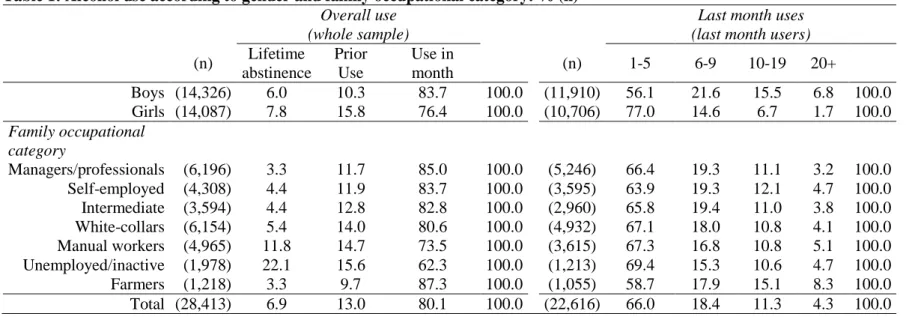
Table 1 shows that lifetime abstinence was reported by 6.9% of the subjects. It was more frequent among the adolescents from manual workers and unemployed/inactive families than among adolescents from the upper occupational categories gathering professionals/managers, self-employed and intermediate occupations (p<0.001), whereas it was much rarer in those from farmers‟ families (p<0.001). Furthermore, the proportion of subjects who experimented alcohol but did not drink during the previous month was higher in the lower categories (p<0.001). Alcohol use in the month prior the survey (80.1% of the sample, n=22,616) was more often reported by adolescents from the farmers than the others (p<0.001) or by those from the upper occupational categories than the others (p<0.001).
When considering last month users, only small differences could be found between occupational categories, although the farmers reported more frequent uses than the others (p<0.001). Differences between boys and girls were relatively small for abstinence, prior use and use in month, but where higher in the upper frequencies of last month use.
Table 2 shows that binge drinking episodes during the previous month (for the individuals who drank alcohol during this period) were more often reported by boys, those from the categories self-employed, farmers, manual workers and unemployed/inactive compared to the others, especially the adolescents from managers/professionals families.
Table 3 shows the results of the multivariate modelling of the overall use adjusted for all covariates using lifetime abstinence as reference. Compared to girls, boys reported less often „prior use‟ (OR=0.86) but reported more often having drank in month (OR=1.26). Except for farmers, all occupational categories reported less often prior use and use in the last month than the managers/professional. Lifetime use and any use in the last month were less frequent in all occupational categories compared to the managers/professionals except the farmers. The differences were especially important for the lower occupational categories.
Table 4 shows the results of the multivariate modelling of last month use adjusted for all covariates. It shows first that the OR for boys increased with the modelled frequency (compared to 1-5 uses), ranging between 2.03 for 6-9 uses and 4.95 for 20+ uses. On one side, compared to managers/professional, white collars, manual workers and unemployed/inactive reported less often 6-9 uses in the last month (OR=0.88, 0.80 and 0.71) and manual workers and unemployed/inactive presented similar odds ratios for 10-19 uses (OR=0.86, 0.78). On the other side, the higher the frequency observed, the higher the OR for the adolescents from farmers families: OR=1.17 (close to significance) for 6-9 uses, 1.79 for 10-19 uses, 3.08 for 20+ uses in the period. Tables 3 and 4 show that the lower categories report less often alcohol use during life and during month than the higher category, whereas it is the opposite among the last month drinkers.
Table 5 shows the results of the multivariate modelling of binge drinking during the previous month for the individuals who drank alcohol during this period, adjusted for all covariates. It shows that boys
were at increased risk for binge drinking, especially for high frequencies (OR ranging between 1.88 and 6.83). The differences between adolescents from any occupational category compared to managers/professionals rise with the frequency of binge drinking episodes. For 1-2 episodes, only the OR for the farmer category was significant (OR=1.23); for 3-5 episodes, were significant those for self-employed, white-collars and manual workers (OR=1.19, 1.16, 1.27) and for farmers (OR=2.14); and for 6+ episodes, the OR for all categories were significant (OR ranging between 1.31 for white-collars and 1.74 for manual workers and 2.96 for farmers). In each occupational category, the ORs were thus rising alongside the level of the outcome variable; furthermore, the confidence intervals of the OR for the levels 1-2 and 6+ were not overlapping for the self-employed, the farmers, the manual workers and the unemployed.
Additionally, we tested whether the interaction of gender with occupational category on one side and with being out of school on the other was not significant in the models of tables 3, 4 and 5 (p-value>0.2 each time), suggesting that the effect of these key variables did not vary significantly with gender.
DISCUSSION
Findings.
This study investigated the associations between parental occupational category and adolescents' patterns of alcohol drinking. It used a cross-sectional survey taking advantage of the representative sampling frame of the National Defense Preparation Day procedure. The sample included over 25,000 French youth, with participation and response rates close to 100%. Several outcomes enabled to consider the type as well as the frequency of use. We found a coherent social pattern linking family occupational category to alcohol use. Compared to managers/professionals, children from unemployed/inactive, manual workers and white-collars' families presented first a lower risk of alcohol use during life or during month; but secondly, among the last month users, children from these categories were less at risk for low levels of use, but showed a similar risk of high levels of use. Thirdly, they also showed much higher risk of reporting high frequencies of binge drinking episodes among last month users. The adolescents from farmers‟ families showed similar risk of alcohol use in
life or in the last month but were at increased risk for frequent levels of alcohol use and binge drinking episodes during the last month. There was no significant interaction between gender on one hand and family occupational category or being out of school on the other, but the gender gap increased markedly with the frequency of use or with the frequency of binge drinking episodes in the last month.
On the one hand, we found that the prevalences and odds ratios for prior use and use of alcohol in the month prior the survey were lower among adolescents from low family backgrounds (especially manual workers and unemployed/inactive categories). Although not investigated in the survey, these results could partly reflect the link between economic background, foreign origins and religion. A significant proportion of unemployed people in France (25%) come from outside the European Union and from Muslim culture (Perrin-Haynes, 2008), the latest known for its strong ban on alcohol consumption. They are also more represented among manual workers. This interpretation was supported by similar results found for alcohol among Asians and Blacks in the US (Ellickson, Dui, Bell, & McGuigan, 1998). On the other hand, a proportion of adolescents coming from the same family occupational categories and who experimented with alcohol are significantly more exposed to the risk of being frequent binge drinkers. This result suggests that adolescents coming from low SES families can schematically be divided into two groups, one of abstainers or episodic drinkers, the other one with higher consumption levels. The pattern of use of this latter group fits well with the strain theory which shows that alcohol intake may be used as a way of coping with stress generated by poor economic opportunities and deprivation (Peirce et al., 1994). Alcohol use of adults may favour that of their children (Chalder et al., 2006), and can also be considered as “rites of passage” yielding better social inclusion (van Gennep, 1960). Alcohol intake may be triggered to gain peers' acceptance, whose behaviours and attitudes toward alcohol are likely to modulate its use as stated by the social learning theory (Borsari & Carey, 2006). Some authors argue that people from disadvantaged backgrounds have fewer and less effective means of assessing the risks and potential health costs of substance intake: they are consequently less receptive to prevention messages while their material difficulties may also result in a short-sighted perspective minimizing the health hazards associated with substance
intake (de Walque, 2007). Our results may reflect a similar situation among adolescents from these social groups.
At the opposite, adolescents from the higher occupational categories (especially from managers/professionals families) present the highest risks of modest levels of alcohol use (lifetime and 1-5 in the month). They present almost similar uses of alcohol uses in the month compared to other categories, but significantly lower risks of frequent levels of binge drinking. It is possible that well-off adolescents present increased risk of accessing alcohol since they declare a more intense, peer-oriented sociability (Peretti-Watel et al., 2006) and have more financial resources at hand that decrease the relative cost of alcohol. This pattern has been found in particular with poor parental monitoring of adolescents' expenditures, and alcohol and substance use in different cultural contexts (Arillo-Santillan et al., 2005; Bellis et al., 2007; Humensky, 2010). At the same time, frequent use is subject to the influence of social and cultural determinants, such as greater knowledge and concern about the negative effects of alcohol abuse (Van Oers et al., 1999) including explicit guidelines for moderate drinking (Neumark, Rahav, & Jaffe, 2003).
Relatively apart when considering lifestyle, housing conditions and economic position, the children of farmers were found to be the most frequent and heaviest drinkers, a result confirmed in general population surveys showing French farmers as regular users (Legleye & Beck, 2007) and more often exposed to chronic alcohol abuse (Com-Ruelle et al., 2008). Similar results have been found in other countries (Oshodin, 1981; Stiernström, Holmberg, Thelin, & Svärdsudd, 1998) and are thought to be linked to cultural and social rather than individual causes, including differences in traditional patterns of socialization, as drinking is a simple and inexpensive pastime and there may be few opportunities for alternative entertainment (Van Hout, 2008). Restructuring in agriculture may also provoke stress from the strain theory perspective, yielding higher alcohol prevalences (Elizabeth, 2007).
Our results are partly corroborated by some studies. Among Mexican adolescents, current drinking (even occasionally) was linked with middle and high tertile of household expenditure (OR=1.26 and 1.32) (Ritterman et al., 2009). This is consistent with our results for episodic uses. But this study provided no focus on indicators of heavier use like binge drinking. Our results are also partly in
agreement with those of Goodman and Huang (2002) who found a negative linear relationship between F-SES and alcohol use. Our results on binge drinking are also consistent with those of Lowry et al. (1996) who found binge drinking to be negatively related to family income. But no study highlighted the positive relationship for light use and negative relationship for heavier use that we found.
Unlike previous studies, we do not confirm the gender-differential social gradient that is known in adults (Casswell, Pledger, & Hooper, 2003; Huckle et al., 2010; Marmot, 1997; Neumark et al., 2003; Van Oers et al., 1999) and in French young adult population (Legleye et al., 2008). Social stratification and environment seemed to play similar roles in the alcohol consumption of boys and girls, despite different levels of use. This may reflect the fact that gender roles socialization, with boys rewarded for risk-taking behaviors, is an ongoing process at this stage of life, especially concerning alcohol use (Martin & Pritchard, 1991).
Apart from the above-mentioned results, our findings are confirmed by those obtained in general population surveys (Bataille et al., 2003; F. Beck, Legleye, Maillochon, & de Peretti, 2008; Bloomfield et al., 2005; Com-Ruelle et al., 2008; Legleye & Beck, 2007). But whether this is in favour of the existence of a process of inter-generational reproduction of alcohol consumption patterns, children of a family being likely to adopt the habits of their parents (Warner, White, & Johnson, 2007), calls for further investigation, as the cross-sectional design used here prevents any causal inference.
Limitations
This cross-sectional survey takes advantage of the sampling frame of the National Defence Preparation Day. The sample is large and representative, with participation and response rates close to 100%. The questionnaire is designed to ensure that it takes about the same time to complete whatever the substance use patterns, which is an added guarantee of confidentiality.
Some limitations arise despite these advantages. First, no question about the consumption of alcohol during the last 12 months was available. As a consequence, it may be that a proportion of experimenters did drink sometimes in this period of time, and it may also be that a proportion of last
month drinkers are in fact experimenters. This may lead to under-estimation of our measures of association and to a lack of statistical power of our study.
The questionnaire lacks explicit questions to assess peer influence on both alcohol initiation (Mundt, 2011) and heavy uses (Fletcher, 2012) as well as parental own alcohol use within households (Warner et al., 2007). Immigrant status and religion of the parents and of the respondents on one side and familial alcohol disorders on the other are important missing variables for our topic (Curran et al., 1999). Other context-related variables are found to influence adolescent alcohol use, such as the density of alcohol outlets (M. J. Chen, Gruenewald, & Remer, 2009), norms regulating the drinking habits of the neighbourhood (Ahern, Galea, Hubbard, Midanik, & Syme, 2008), or related to area-level socioeconomic status (Karriker-Jaffe, 2011). We do not have any measure regarding adolescents‟ personality and mental health, which can mediate the association between family SES and alcohol use and abuse. Moreover, the cross-sectional design does not enable us to determine the age at which social differentiation in alcohol use occurs; for the same reason it may also be the case that dropout follows alcohol abuse.
The occupational category of each parent may be misclassified by adolescents, due to ignorance or social desirability bias. We did not ask for income or educational level of the parents, although they enter the concept of SES, because they are rarely accurately known by the adolescents. They are very strongly linked to occupational category in France (Chauvel, 1999; Derosières & Thévenot, 2002), and typologies based on the parents' occupations reported by the adolescents have been validated and judged reliable (Lien, Friestad, & Klepp, 2001). Although mother's and father's occupations could have different influences, we considered only the highest one in order to provide a simple indicator. There was no special assessment for the adolescents whose parents are divorced, as in practice both parents are financially contributing to their needs. Finally, we could not take the past occupational category of the retired persons into account. But because the respondents were 17, the retired persons were only a small group (3.9% among the fathers, 1.3% among the mothers) with reduced potential bias.
Recently, measures of subjective socioeconomic status have been developed that compare oneself or one's family to the others (Goodman et al., 2001), showing different results compared to objective scales for tobacco use (Finkelstein, Kubzansky, & Goodman, 2006) and for alcohol and tobacco use (Ritterman et al., 2009). These indicators may be particularly useful for adolescents who have a different perception of socioeconomic status than adults, and who respond to the economic status of their peers in a very sensitive manner. Although the concept of social hierarchy used in instruments designed for adults is generally well understood (Adler, Epel, Castellazzo, & Ickovics, 2000; Demakakos, Nazroo, Breeze, & Marmot, 2008), this is not the case in the most widely used instrument designed for adolescents (Goodman et al., 2001): it mixes financial, occupational and prestige aspects as well as school aspects (respect, grades and involvement in extracurricular activities) that raise important conceptual difficulties in understanding and translation (Ritterman et al., 2009).
Conclusion.
According to Barnett‟s terminology (Barnett, Whiteside, Khodakevich, Kruglov, & Steshenko, 2000), adolescents from the least affluent families appeared less „susceptible‟ to drink alcohol, but potentially more „vulnerable‟ to problems because they showed more often intensive uses.
Previous literature has underlined the consequences of alcohol misuse during youth, including acute effects like early, unprotected sexual intercourse (Brown & Vanable, 2007; Sivaram et al., 2008), violence and antisocial behaviour (Rodney, Rodney, Crafter, & Mupier, 1999), car driving under the influence of alcohol and fatal crashes (Eenso, Paaver, Harro, & Harro, 2005; Laumon, Gadegbeku, Martin, & Biecheler, 2005), school problems such as poor academic achievement (Aertgeerts & Buntinx, 2002), grade retention (Rodney et al., 1999), school dropout (Chatterji & DeSimone, 2005) and late graduation (Renna, 2007). Previous studies also underlined long term consequences of intense alcohol use in adolescence such as strong negative developmental outcomes (Masten, Faden, Zucker, & Spear, 2008), later problematic alcohol use (Poikolainen, Tuulio-Henriksson, Aalto-Setala, Marttunen, & Lonnqvist, 2001) and which are related to later higher unemployment risks (Ellickson, Tucker, & Klein, 2003).
Albeit offering valuable paths to improve prevention, very few of these studies considered the respondents' socioeconomic status. Our results suggest that prevention strategies should focus on the populations from low SES background and also on adolescent from farmers families in order to prevent the widening of social inequalities that may be further aggravated by untargeted prevention (Frohlich & Potvin, 2008; Lombrail, 2007). However, additional research is needed to identify the factors that hinder or favour progression in alcohol use among adolescents from families of high and low occupational categories.
Acknowledgements.
This study was funded by the French Monitoring Centre on Drugs and Drug Addictions (OFDT), who provided financial support for the conduct of the survey and the writing of this paper.
Conflict of interest.
Table 1: Alcohol use according to gender and family occupational category: % (n)
Overall use (whole sample)
Last month uses (last month users)
(n) Lifetime abstinence Prior Use Use in month (n) 1-5 6-9 10-19 20+ Boys (14,326) 6.0 10.3 83.7 100.0 (11,910) 56.1 21.6 15.5 6.8 100.0 Girls (14,087) 7.8 15.8 76.4 100.0 (10,706) 77.0 14.6 6.7 1.7 100.0 Family occupational category Managers/professionals (6,196) 3.3 11.7 85.0 100.0 (5,246) 66.4 19.3 11.1 3.2 100.0 Self-employed (4,308) 4.4 11.9 83.7 100.0 (3,595) 63.9 19.3 12.1 4.7 100.0 Intermediate (3,594) 4.4 12.8 82.8 100.0 (2,960) 65.8 19.4 11.0 3.8 100.0 White-collars (6,154) 5.4 14.0 80.6 100.0 (4,932) 67.1 18.0 10.8 4.1 100.0 Manual workers (4,965) 11.8 14.7 73.5 100.0 (3,615) 67.3 16.8 10.8 5.1 100.0 Unemployed/inactive (1,978) 22.1 15.6 62.3 100.0 (1,213) 69.4 15.3 10.6 4.7 100.0 Farmers (1,218) 3.3 9.7 87.3 100.0 (1,055) 58.7 17.9 15.1 8.3 100.0 Total (28,413) 6.9 13.0 80.1 100.0 (22,616) 66.0 18.4 11.3 4.3 100.0 Chi-square p-value for the association of family occupational category and both Overall use and Last month uses<0.001
18
Table 2: Frequencies of binge drinking in the last month according to family occupationalcategory among last month users: %, (n)
(n) 0 episode 1-2 episodes 3-5 episodes 6+ episodes Boys (11,910) 29.7 36.4 20.4 13.5 100.0 Girls (10,706) 50.6 35.1 10.5 3.8 100.0 Managers/professionals (5,246) 43.2 36.4 14.1 6.4 100.0 Self-employed (3,595) 37.0 36.0 17.1 10.0 100.0 Intermediate (2,960) 40.4 36.4 14.9 8.3 100.0 White-collars (4,932) 39.7 36.3 15.8 8.2 100.0 Manual workers (3,615) 37.7 34.5 16.7 11.1 100.0 Unemployed/inactive (1,213) 38.3 34.3 15.3 12.1 100.0 Farmers (1,055) 35.6 33.2 19.1 12.1 100.0 Total (22,616) 39.6 35.7 15.8 8.9 100.0
Chi-square p-value for the association of family occupational category and frequency of binge
drinking episodes<0.001
19
Table 3: Odds ratios and 95% confidence intervals for overall use: prior alcohol use in life and alcohol use in the last month opposed to lifetime abstinence (generalized logistic regression)Lifetime
abstinence Prior use Use in month
reference OR 95%CI OR 95%CI
Boys (ref=girls) 1 0.86* 0.76-0.97 1.26*** 1.13-1.44
Family occupational category
Ref=managers/professionals 1 1.00 1.00 Self-employed 1 0.70** 0.56-0.90 0.60*** 0.48-0.74 Intermediate 1 0.78* 0.60-0.99 0.67*** 0.53-0.84 White-collars 1 0.67*** 0.54-0.83 0.50*** 0.42-0.61 Manual workers 1 0.32*** 0.26-0.39 0.19*** 0.16-0.23 Unemployed/Inactive 1 0.17*** 0.13-0.21 0.08*** 0.06-0.10 Farmers 1 0.84 ns 0.55-1.27 1.05 ns 0.72-1.52
OR are adjusted for: daily tobacco smoking, any cannabis use in the last month, lifetime use of any other illicit drug, being out of school, socializing, parental separation.
*, **, ***, ns: Wald-Chis-square test p-value <0.05, 0.01, 0.001 and not significant. Significant OR are in bold type.
20
Table 4: Odds ratios and 95% confidence intervals for the frequency of alcohol use among last month drinkers (generalized logistic regression)1-5 uses 6-9 uses last month 10-19 uses last month 20+ uses last month
reference OR 95%CI OR 95%CI OR 95%CI
Boys (ref=girls) 1 2.03*** 1.89-2.19 3.13*** 2.84-3.45 4.95*** 4.21-5.83
Family occupational category
Ref=managers/professionals 1 1.00 1.00 1.00 Self-employed 1 0.91 ns 0.81-1.03 0.97 ns 0.84-1.12 1.18 ns 0.94-1.48 Intermediate 1 0.98 ns 0.86-1.10 0.97 ns 0.83-1.14 1.06 ns 0.83-1.36 White-collars 1 0.88* 0.79-0.98 0.90 ns 0.79-1.03 1.07 ns 0.86-1.33 Manual workers 1 0.80*** 0.71-0.90 0.86* 0.74-0.99 1.22 ns 0.97-1.52 Unemployed/Inactive 1 0.71*** 0.59-0.85 0.78* 0.62-0.98 1.13 ns 0.82-1.56 Farmers 1 1.17 ns 0.97-1.41 1.79*** 1.44-2.12 3.08*** 2.30-4.12 OR are adjusted for: daily tobacco smoking, any cannabis use in the last month, lifetime use of any other illicit drug, being out of school, socializing, parental separation.
*, **, ***, ns: Wald-Chis-square test p-value <0.05, 0.01, 0.001 and not significant. Significant OR are in bold type.
21
Table 5: Odds ratios and 95% confidence intervals for binge drinking episodes in the last month among last month drinkers (generalized logistic regression)0 1-2 episodes 3-5 episodes 6+ episodes
ref OR 95%CI OR 95%CI OR 95%CI
Boys (ref=girls) 1 1.85*** 1.73-1.98 3.68*** 3.35-4.03 6.86*** 6.02-7.80
Family occupational category
Ref=managers/professionals 1 1.00 1.00 1.00 Self-employed 1 1.03 ns 0.93-1.15 1.19* 1.03-1.38 1.49*** 1.24-1.79 Intermediate 1 1.06 ns 0.95-1.18 1.14 ns 0.97-1.33 1.33** 1.09-1.63 White-collars 1 1.03 ns 0.94-1.14 1.16* 1.01-1.32 1.31** 1.09-1.36 Manual workers 1 1.00 ns 0.89-1.10 1.27** 1.10-1.47 1.74*** 1.45-2.09 Unemployed/Inactive 1 0.88 ns 0.74-1.04 1.02 ns 0.82-1.26 1.65*** 1.27-2.14 Farmers 1 1.23* 1.04-1.46 2.14*** 1.72-2.66 2.96*** 2.25-3.88 OR are adjusted for: daily tobacco smoking, any cannabis use in the last month, lifetime use of any other illicit drug, being out of school, socializing, parental separation.
*, **, ***, ns: Wald-Chis-square test p-value <0.05, 0.01, 0.001 and not significant. Significant OR are in bold type.