Essays on Credit Risk
A dissertation presented by
Matteo Borghi
Supervised by
Prof. Giovanni Barone-Adesi
Submitted to the
Faculty of Economics
Università della Svizzera italiana
for the degree of
Ph.D. in Finance
Contents
Introduction . . . 4
Systematic and specific risk in the CDS market. . . 8
Structural Credit Risk Models in presence of Observational Noise . . . 54
Liquidity and Limits of Arbitrage in Structural Credit Risk Models . . . 99
Conclusion . . . 128
Introduction
The research consists of two major topics. The first one is related to reduced-form credit risk models and in particular identifies an idiosyncratic and a sys-tematic component in Credit Default Swap returns. The remuneration for the undiversifiable component is therefore estimated. The second topic consists in a deep analysis of structural credit risk models, with a specific focus on the reasons for their failure in the explanation of observed credit spreads, both in levels and in differences. This issue is tackled from two different perspectives: corporate bonds and CDS. The following three chapters will be part of the research.
In the first chapter, we study the role of systematic risk in the credit market and in CDS spreads in particular. The studied variables are the mark-to-market returns of a protection-seller of CDS contracts on a set of investment grade firms. A simple linear market model is proposed to describe the returns of the single CDS contracts using the market index (CDX index) as a systematic factor. The ability of the systematic factor to price CDS in the cross section dimension is also assessed. Consequently, the risk premium per unit of systematic risk is computed and compared to previous studies. Also the evolution through time of the performance of this simple linear model is investigated, with a specific focus on the behaviour during the financial crisis. Furthermore, a decomposi-tion of the risk between systematic and specific is proposed and the changes in the proportion of the two, both on the entire distribution and on the tails, is investigated. Finally, a decomposition between specific and systematic risk is investigated for every different industrial sector. The previous literature dis-covered a common systematic factor in credit returns (see e.g. Collin-Dufresne et al. (2001) or Berndt and Obreja (2010)). In this work we propose a simple framework to model this common factor and verify if it is actually priced by the market.
In the second chapter the most important structural credit risk models are studied in the framework of a state-space framework. In particular, all the structural models can be represented in a state space form, where the unob-served variables are asset values and asset volatilities. Such latent quantities are measured, possibly with an additional noise, by two observed quantities: equity prices and volatilities implied in equity options. In general the mea-surement equations are nonlinear and therefore, in place of a standard Kalman
filter, some nonlinear filtering techniques are required in order to eliminate the observational noise. In the work we verify to which extent such sophisticated filtering approach outperforms simple numerical inversion of measurement equa-tions, performed under the hypothesis of absence of observational noise.
One of the testable implications of the presence of observational noise con-taminating the measurement equations is the better performances of the filtering technique in periods of stress, when liquidity and limits of arbitrage may induce strong deviations of equity prices and volatilities from the theoretical values implied by their assets. This difference between the pre- and post-crisis pe-riod is actually observed and supports the presence of observational noise. The improvement given by the use of bivariate state space models (based on both equity prices and volatilities) with respect to a univariate one, already proposed in the literature, is also investigated.
On the common ground given by bivariate state space models, a comparison between the performance of the most commonly used structural models is per-formed. In particular, the ability to explain observed CDS spreads is studied. The considered models are the simple Merton’s Model, the extension to stochas-tic interest rates, the endogenization of the default threshold and the inclusion of a jump component in the stochastic process for the latent asset values. The improvement given by stochastic interest rates and endogenous default, per se, is not substantial. Only the introduction of jumps is able to reduce the differ-ence between predicted and observed spread. Finally, the jump risk premium implied in credit spreads will be investigated and a decomposition of the default intensity between a jump and a diffusion-to-default component will be analyzed. The study enlarges the literature about the empirical testing of structural credit risk models (such as Jones et al. (1983), Huang and Huang (2003) and Eom et al. (2004)). Furthermore, we extend the use of the state space framework for the estimation of structural credit risk models. This idea has been proposed by Duan and Fulop (2009) in the univariate case and we extend it to the case of two latent state variables.
The last chapter extends the study of the performances of structural credit risk models using a large dataset of actual execution prices of more than 4.000 corporate bonds along ten years. The main objective is to verify the role of market-specific liquidity measures and market-wide indicators of limits of ar-bitrage in the explanation of the errors made by structural models. The equi-librium between the market values of assets and all types of liabilities, and therefore the accuracy of structural models, are guaranteed by non-arbitrage re-lationships. Therefore, in periods of adverse liquidity conditions and/or strong limits to arbitrage forces, the performances of structural models are supposed to deteriorate. We assess the performances of structural models by verifying the ability of stock and implied volatility returns to explain the changes in credit spreads. In a second step, we verify the dependence of the errors left by structural models on the liquidity measures specific to the two markets involved in the non-arbitrage relationships, i.e. the equity and corporate bond market. If the performances of structural models were affected by liquidity conditions, then one would expect higher errors in presence of adverse liquidity conditions.
The errors of structural models are actually found to significantly depend on liquidity indicators, and in particular from the liquidity conditions in the credit rather than in the equity market. Furthermore, if also limits of arbitrage have a role in the poor performance of structural models, then the residuals left by both structural variables and liquidity indicators should significantly depend on market-wide indicators of restriction to arbitrage forces. Also this prediction is verified since the average errors of structural models are found to depend on market-wide liquidity indicators such as the TED and LIBOR-OIS spread.
The work relies on the empirical testing literature mentioned in chapter two and extends it identifying some specific drivers that describe the underperfor-mance of structural credit risk models.
Systematic and specific risk in the CDS market
Giovanni Barone-Adesi Matteo BorghiAbstract
In this paper we study the role of systematic risk in the credit market and in CDS spreads in particular. We propose a simple linear market model to describe the returns of the single CDS contracts using the market index (CDX index) as a factor. In the cross section dimension, the CDX factor is priced and a significant risk premium of 37 basis points is estimated and seems to be compatible with previous studies. However this simple model does not seem to be enough to describe the entire cross section of realized returns since a significant intercept is present, especially during the crisis period. We also study the evolution of systematic risk before and after the financial crisis. Systematic risk seems to considerably increase during the crisis when measured by
the average R2 of time series regressions, the variance explained by
the first principal components and the increase in the extreme tail dependence. Finally we propose a simple decomposition of the variance to separate the systematic and specific component. A strong increase in the systematic fraction is observed during the crisis. The sector with the highest systematic fraction of variance, and therefore highest sector fragility, is the financial one.
1
Introduction
During the recent financial crisis, we observed a dramatic increase in the credit spreads quoted on the market. This is true for both the spreads implicit in the corporate bond market and those paid to buy protection in the CDS market. This rise in the spreads can be interpreted as an increase in the risk neutral default probability of the considered companies since such a dramatic change in the expected recovery rate does not seem plausible. One first question that arises is therefore whether such high values of the default probability can be considered systematic or specific and thus diver-sifiable. Another question concerns the change in the role of systematic components of credit risk during the crisis period. We investigate such ques-tions in the CDS market. This choice is justified by the high liquidity of the credit derivatives market and by the huge volume of outstanding contracts. According to the ISDA Market Survey of June 2010, the total outstanding notional covered by CDS contracts amounts to more than 26 trillions in the first half of 2010. Although this number is huge, it is well below the historical maximum of outstanding notional, which is equal to more than 62 trillions in the second half of 2007. Another justification of the choice can also come from the wider and wider use of indexes of CDS contracts. Here we focus only on the US market and consider only the CDX as a comprehensive index. The first contribution of the paper is therefore to propose a model that separates the systematic and specific components of risk in the CDS market. The second objective is to analyze in depth the evolution of systematic credit risk before and during the financial crisis. This is done both on the entire sample of firms and considering the same data grouped by sector. The change in risk is investigated also with respect to the “extreme systematic” risk, measured in terms of extreme tail dependence.
The remainder of the paper is organized as follows. In section 2 we briefly review the literature on the topic. In section 3 we describe the data we are using with some of its most important statistical properties. In section 4 we propose a statistical characterization for the single CDS returns based on a linear dependence on the returns of the CDX market index. In section 5 we present the results of the estimated model in the time series and cross-section dimension, in section 6 we show some tests for the linear model and finally in section 7 we decompose credit risk into its two components. Section 8 concludes.
2
Review of the literature
In this paper we rely on several different strands of literature. Since we are applying a linear model for the characterization of returns, we rely first of all on the classical asset pricing literature related to the Capital Asset Pricing Model such as Sharpe [1964], Lintner [1965] and Mossin [1966]. Nevertheless the classical CAPM literature is based on the equilibrium condition in capital markets. Given the fact that here we are considering only a relatively small segment of the entire financial market (the credit market), it seems inappropriate to invoke such a strong condition. Therefore we are simply assuming that the returns in the credit market are linearly dependent on the returns of a (sufficiently diversified) credit market index and that pricing in this market can be done relying only on the (weaker) non-arbitrage condition. This statistical characterization is analogous to the Arbitrage Pricing Theory usually applied to the equity market, whose literature is originated by the works by Ross [1976] and Roll and Ross [1980].
The second big strand of literature is obviously referred to credit risk. As is well known, we can identify two big families of credit risk models: structural and reduced-form. In this paper we are directly modeling credit spreads, neglecting in this way all the other corporate and market information available to agents and thus assuming that all the relevant information is efficiently incorporated into observed credit spreads. Thus the literature we are mainly referring to is the one of reduced-form models. The first two articles in this group are Altman [1968] and Beaver [1968]. In both cases, the default probability is directly modeled through the use of balance-sheet variables. The first examples of reduced-form models based on market data, instead, are in Jarrow and Turnbull [1992] and Jarrow and Turnbull [1995]. A more recent reference for reduced-form models is Duffie and Singleton [1999]. In all the last three articles the relevant variable is the intensity (Hazard Rate) of a stochastic process that models the arrival of default events.
A number of articles directly address the modeling of credit spreads
through the use of a set of explanatory variables. Among these,
it is worth mentioning Collin-Dufresne, Goldstein, and Martin [2001], Ericsson, Jacobs, and Oviedo [2009] and Berndt and Obreja [2010]. The first article shows that the variables used in structural models (e.g. implied volatility or leverage) have a relatively small explanatory power on corpo-rate bond premia and that a strong systematic factor is still present in the residual of these regressions. The second article reaches a very different conclusion, showing that volatility, leverage and risk-free rate explain quite well CDS spreads and leave no systematic factor in the residuals. However, this second study is performed on a much shorter time series and CDS spreads are used in place of corporate bond spreads. Finally, the article
by Berndt and Obreja [2010] tries to explain the residual common factor found by Collin-Dufresne et al. [2001] building a “catastrophic factor” as the difference between the spreads of tranches with different seniority in CDO products. Such factor actually seems to be strongly significant and to eliminate the common behaviour in model residuals.
There is also an increasing literature that investigates the presence of
a systematic risk and fragility factors in credit markets. First of all,
Jarrow, Lando, and Yu [2005] theoretically discuss the equivalence between the risk-neutral and physical measure showing that the two measure are asymptotically equivalent for “well diversified portfolios”. An exact equiva-lence is based on stronger utility arguments. Das, Duffie, Kapadia, and Saita [2007] verify that the correlation between defaults is higher than can be ex-plained using observable factors. They argue that an economy-wide frailty factor is present that makes default events more correlated. A similar finding is presented by Duffie, Eckner, Horel, and Saita [2009]. They show that the high value of extreme correlation in defaults can be explained introduc-ing a common unobserved systemic factor. In this case they also estimate this latent factor as a component in the default intensity process. Finally Bhansali, Gingrich, and Lonstaff [2008] estimate a model in which the de-fault intensity is a linear combination of three latent Poisson processes. The first corresponds to specific default risk, the second to the risk of a sector-wide default and the third to systemic risk. We also have to consider the literature on systematic risk which is more closely related to linear models such as Sharpe [1963].
A strand which is related to these articles is the one that investigates the presence and the size of a risk premium for undiversifiable credit risk. In Fama and French [1989] a systematic undiversifiable risk in corporate bonds is identified, which can be partially explained using macro variables and indicators of the business cycle in particular. Also Duffee [1999] verifies the presence of a positive price for credit risk. In this case it is estimated from the intensity of the arrival of defaults, which is modeled as a square root diffusion process. The same result is also found by Elton, Gruber, Agrawal, and Mann [2001] and Liu, Longstaff, and Ravit [2002]. In this last case the estimation of the premium is based on the Interest Rate Swap market, in which a default risk of the counterparty is implicit.
Other articles define the risk premium as the ratio between risk-neutral and physical default probabilities. This measure, which is indeed proportional to the state price per unit probability, can be interpreted as the premium required by a risk averse agent buying credit risk. This measure is used among others by Berndt, Douglas, Duffie, Ferguson, and Schranz [2004] and Driessen [2005]. In the first case an estimation of the physical default probability is obtained using the Expected Default Frequencies from the
KMV model, while in the second case the actual default frequencies from Moody’s and S&P are used. In all the mentioned articles a ratio of roughly 2 is obtained. Finally it is worth citing the articles by Hull, Predescu, and White [2005] and Lonstaff, Giesecke, Schaefer, and Strebulaev [2010]. In both cases the premium is estimated from corporate bond prices and is significantly different from zero. The only article in contrast with this literature is Dichev [1998], in which no positive relationship between default risk (measured by Altman [1968] Z-Score and Ohlson [1980] model) and subsequent returns is found. Therefore this last work is the only which finds no remuneration for bearing default risk.
3
Data
3.1 The CDX index
As a proxy for the systematic credit risk, we use the Markit CDX index Investment Grade with maturity 5 years. This is calculated as the average of the CDS spreads of the most liquid 125 reference entities. In order to eliminate the spreads of firms that have been downgraded, for which a credit event took place and the ones that are not sufficiently liquid any more, the CDX index rolls its constituents every six months. The continuous series of CDX spreads provided by Bloomberg do not account for the variation in the spread simply due to the roll over and only continue the series with the spread of the new on-the-run series. The series used here, on the other hand, concatenates the percentage changes of the 15 on-the-run series, removing in this way the spurious variation only due to the roll over. The source is in this case Bloomberg.
The time period considered here coincides with the existence of the CDX index. It begins in October 2003 and ends in September 2010. All the following analysis is based on a measure of the performance realized by a potential investor that sells protection in the CDS or CDX market. Such performance is computed accordingly to the ISDA Standard Model explained in detail in Appendix and is expressed in percentage of the standard notional amount of the contract. In general, very similar results are obtained when the simple first difference of the series is used in place of returns.
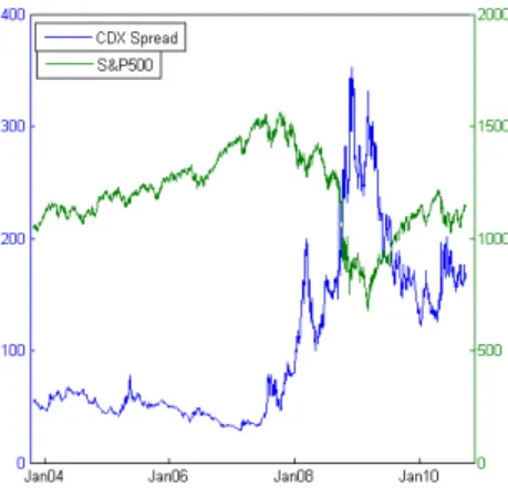
The considered period is a very particular one and includes the heavy credit crisis of 2008-2009. The evolution of the CDX spread is represented in figure 1 together with the evolution of the S&P500 Index.
It’s easy to verify the sharp increase in CDX spread and the corresponding fall of the stock market starting in August 2007. This close relationship is confirmed by a negative correlation between the two series of returns equal
to -45.16% and -60.16% for the daily and two-weeks returns respectively. We also split the considered time period into two subperiods of equal length, the first goes from October 29, 2003 to April 13, 2007 and the second from April 16, 2007 to September 30, 2010. As far as daily changes are concerned, the correlation increases in absolute value from -0.3494 in the first period to -0.4615 in the second, as one might expect in periods of crisis.
In table 3.1, we present some descriptive statistics of the daily time series of the CDX spread in levels.
N Mean St. Deviation Min. Median Max.
CDX Index 1807 102.98 74.21 28.48 60.95 352.60
Table 1: Descriptive statistics
The minimum has been reached in February 2007 and the maximum in December 2008.
We tested the null hypothesis of unit root of the CDX spread process using an augmented Dickey-Fuller test. The null hypothesis cannot be rejected at all the standard confidence levels (the ADF t-statistic is -2.34). The CDX spread process therefore seems to be non-stationary. The same result is confirmed by the Phillips-Perron and the KPSS test.
If we consider the first difference of the process, the null of unit root is rejected at any confidence level (the ADF t-statistic is -27.47). We can conclude that the series is integrated of order 1.
We also investigated the Granger causality relationships between equity market (here represented by the S&P 500 Index) and the credit market (CDX Index) using again daily data. The strength of results partially depends on the number of lags we use in the vector autoregression model. However we observe in general a strong causality from the equity market to the CDX market. In particular granger-causality probabilities are virtually zero in this direction, so that we can always reject the null that Equity market does not cause (in a Granger sense) Credit market. In the opposite direction the causality relation depends on the number of lags used but in general it seems much weaker. For example, the Granger causality probabilities with 5 lags (one week) are the following.
Variable CDX S&P 500
CDX 0.0000 0.0000
S&P 500 0.0412 0.0003
Table 2: Granger Causality probabilities between CDX and S&P500 We can see that at 5% confidence level we can always reject the null of
absence of causality in both direction but at 1% level causality is rejected only from the CDX to the S&P 500 but not in the opposite direction. We also investigated the cointegration between the time series of the CDX spread and the S&P500. Both the CDX index and the S&P 500 are inte-grated of order 1. Since we are considering only two variables, we can test cointegration by simply implementing the two step Engle-Granger proce-dure. After estimating a regression on the two variables in levels, we use the augmented Dickey-Fuller test on the residuals to verify their stationarity. The unit root hypothesis in the residuals can never be rejected. Therefore no strong cointegration relation between the S&P 500 and the CDX spread is present. The test based on Johansen procedure gives the same result accepting the null of no cointegration relations. This seems quite reasonable since we expect the equity index to be much more persistent than the CDX. The latter, although statistically I(1), from an economic point of view can show a behaviour closer to stationarity. This fact prevents the existence of a long-term equilibrium relationship between the levels of the two series. We also briefly investigate the process of price discovery between stock and credit market. In the literature, such task is achieved using the measure introduced in Gonzalo and Granger [1995], and more recently applied by Blanco, Brennan, and Marsh [2005] in the credit spreads context, or by means of the intervals proposed by Hasbrouck [1995]. Unfortunately in our case both these procedures are not applicable since the time series of CDX and S&P500 index are not cointegrated.
Therefore, we simply verify the dependence of contemporaneous returns of the CDX index on lagged returns of the S&P500 index and vice versa. We consider only the most significant lags, that is the first two. The two equations we are estimating are the following
rCDX,t=b0+b1rSP,t−1+b2rSP,t−2+ε1,t (1)
rSP,t=c0+c1rCDX,t−1+c2rCDX,t−2+ε2,t (2)
whererCDX,t−k andrSP,t−kare the CDX and S&P500 index return respectively, at the kth lag. The results are the following
Coefficient t-stat
b0 -2.779e-05 -0.5760
b1 0.0396 11.0623
b2 0.0199 5.5442
Coefficient t-stat
c0 3.1801e-05 0.0996
c1 -0.2920 -1.9263
c2 -0.2594 -1.7110
Table 4: Estimated coefficients of equation (2)
We can see that the S&P500 index actually anticipates the CDX index both at lag 1 and at lag 2. The significance of the first lag is also noticeable. On the other hand there is no economic significance in the negative coefficients of the second estimation, in which the ability of CDX index to anticipate S&P500 is assessed. We can conclude that the credit market can be predicted using information from the equity market while the opposite is not true, at least in the considered sample. This is also fully consistent with the results about Granger causality exposed above. A reason for this could be the presence of more “informed traders” in the equity than in the credit derivatives market, which induces a delay in the complete incorporation of the information in credit market prices. Also this result can be interpreted as a lack of efficiency in the credit market. It is quite surprising to observe such a dependence on a daily horizon, given that one would expect the information to flow from a market to another on an intraday horizon. A similar result, but referred to corporate bonds, is obtained by Kwan [1996], who shows that equity market actually anticipates the corporate bond market, supporting the hypothesis that more informed traders are present in the equity market.
A simpler alternative explanation of this finding can come from the presence of stale quotes in the CDS contracts underlying the CDX index which automatically induces correlation between the CDX index and lagged equity returns.
According to standard structural models (such as Merton [1974]) another determinant beyond equity value affects the default event: volatility. In figure 2 we represent the evolution of the VIX and CDX Index. The common trend is evident and it is also confirmed by the correlation between the two series, which is equal to 39.41% for daily changes and 56.48% for two-weeks changes. Also in this case, the correlation in the second subperiod (40.39%) is higher than in the first (33.37%).
We also compared the behaviour of the CDX index and traditional bond indexes. In particular we built an artificial index as the difference between daily returns in the Citigroup GBI Corporate BBB 1-5 Years and the Citi-group GBI Treasury 1-5 Years. The daily returns of the resulting index have a correlation equal to 62.51% with the CDX Index. This indicates that the spreads on the bond and credit derivative market are highly but not perfectly correlated. Of course, in this case, the imperfect correlation can also come
from different maturity (5 years Vs. 1-5 years) and rating.
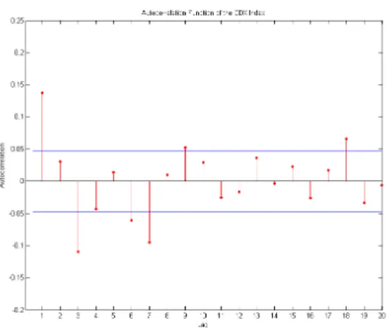
Finally, we consider the returns of the CDX index at 1-day frequencies. For the computation of such returns refer to section A. The first interesting result, as already documented in Bystrom [2008] for the Itraxx indexes, is the presence of a strong autocorrelation (13.91%) in the first differences of the daily CDX spreads. The same result (13.7%) is obtained when we use the daily mark-to-market returns of the market value of a CDX contract expressed as a percentage of the notional. Some autocorrelation (3.21% and 3.06% for the first differences and the mark-to-market percentage variations respectively) is present also at the second lag.
We verify this by estimating the following simple AR(2) model
∆CDXt=a0+a1∆CDXt−1+a2∆CDXt−2+εt (3)
and we get the coefficients in table 5.
Coefficient t-stat
a0 0.0512 0.4563
a1 0.1373 5.8285
a2 0.0130 0.5502
Table 5: Estimated coefficients of equation (3)
The results are very similar when we use the percentage mark-to-market returns in place of the simple first difference. The regression coefficient is still strongly significant.
We also evaluated the evolution in time of such autocorrelation. In partic-ular, we evaluate it in the two subperiods defined above. The first order autocorrelation is significantly higher in the first period (21.69%) than in the second (13.56%). Similar results are derived from the estimation of equation (3). In particular
10/2003-7/2007 7/2007-9/2010
Coefficient t-stat Coefficient t-stat
a0 -0.0170 -0.5615 0.1223 0.5491
a1 0.2169 6.5041 0.1356 4.0631
a2 0.0276 0.8271 0.0123 0.3692
Table 6: Estimated coefficients of equation (3)
In both periods the lagged difference is statistically significant but the coefficient and its significance is reduced in the second period.
Also in this case, this apparent inefficiency can be justified by the presence of stale quotes in the CDX index and in particular in the early stages of its life, since this phenomenon is vanishing as the volume of transactions and the number of agents in the market is increasing.
Of course this analysis is based on quoted mid prices and does not consider the presence of bid-ask spreads and the costs required to implement an arbitrage strategy between the index and the single CDS.
The most important descriptive statistics of the time series of daily CDX returns are summarized in the following table.
N Ann. St. Dev. Skew. Kurt. Min. Max.
CDX Index 1806 3.33% -0.7024 22.51 -2.15% 1.55%
Table 7: Descriptive statistics for the CDX Index
It’s important to notice the strong negative value of the skewness, especially if compared with the skewness of the S&P500 index in the same period, which is -0.2622, and the extremely high level of kurtosis. The distribution of CDX returns is very far from normality and the Jarque-Bera null hypothesis of normality is strongly rejected (with a p-value of less than 0.001).
If we extend the horizon and consider the 15-days differences and returns the presence of autocorrelation completely disappears. Only a negative autocorrelation of about 2% is present for the first and second lag. The estimation of equation ((3)) for 15-days differences and mark-to-market variations gives in this case totally insignificant coefficients (not reported). The entire autocorrelation function of daily returns is represented in figure 3 and shows a strongly significant coefficient at the first lag.
If we move to the autocorrelation function of squared returns, we can deduce the clear presence of strong persistence in variance (see figure 4). So, in analogy to the equity market, we can hypothesize the presence of a GARCH structure also in the returns from credit default swap market. There are no dramatic differences between the particular specifications of the GARCH model. We explored the use of different specifications such as the EGARCH and the Glosten-Jagannathan-Runkle (GJR), and different distributions for the innovations such as Normal and Student’s t, but the improvement in the fit of the data is not decisive. Also concerning the choice of ARCH and
GARCH parameters the simplest choice of p = q = 1 seems to be enough.
Therefore, in figure 5 we present the autocorrelation function of the filtered residuals of a parsimonious GARCH(1,1) model. Much of the structure of the returns is removed and residuals are quite close to serial uncorrelation. Unfortunately, this procedure doesn’t have a particular impact on the
normal-ity of returns. In fact the values of skewness and kurtosis are not significantly modified with respect to the non-filtered series and the Jarque-Bera hy-pothesis of normality is still strongly rejected (with a p-value still less than 0.001).
3.2 A Markov Switching model
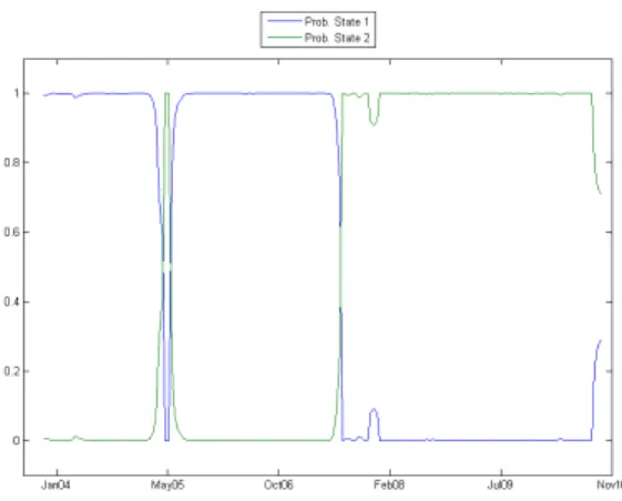
We have already mentioned the apparent presence of two clearly separated time periods in the considered interval. In particular, the first “State of the World” ends at the beginning of the sub-prime crisis in the summer of 2007 while the second goes from the beginning of the crisis to the end of the period. We consider such a separation several times in the paper. We now investigate the statistical reliability of our choice. In order to do so, we fit a two-state Markov switching model on the time series of returns for the CDX index.
We can clearly fit a two states model and observe a neat break between state 1 and 2 in the summer of 2007. The first of the two states is characterized by credit returns with a slightly higher mean and a much smaller variance. The graph of the time series of the (smoothed) probabilities of being in state 1 or 2 is presented in figure 6. We observe the apparent change of state during the summer of 2007 and a smaller switch to the “bad” state around May 2005. We can identify this episode with the automotive sector crisis, and in particular with the downgrade of GM bonds from investment grade to junk, which had an impact on the entire credit market.
This finding confirms the presence of a Markov switching model in the credit market already investigated by Alexander and Kaeck [2008] for the iTraxx index in the European market.
3.3 Single CDS contracts
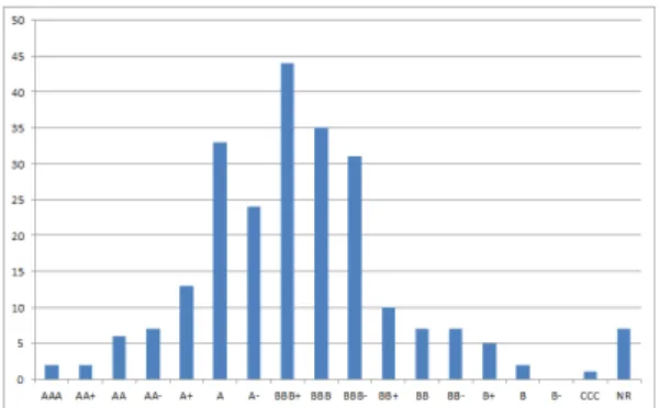
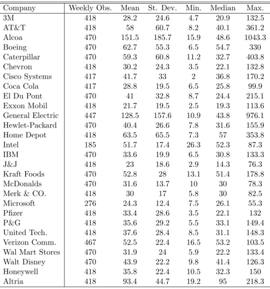
The CDS spreads used here are relative to 5-years contracts on 238 reference entities. These companies are selected from the population of the S&P500 based on the liquidity of the quoted CDS spreads. All the spreads used are quoted and not transaction spreads and the source is Thompson Datastream. In figure 7 we represent the rating distribution of the sample as provided by S&P and observed at the end of the period.
The median rating is BBB+. One has to consider that these ratings are observed after the financial crisis of 2008 and 2009. Consequently, they are arguably lower than the ratings of the same companies at the beginning of the period.
The distribution by GICS sector of the companies is the following GICS Sector N Materials 21 Industrials 34 Consumer Discretionary 42 Telecommunication 10 Energy 23 Consumer Staples 25 Financials 31 Utilities 19 Information Technology 12 Health Care 21
Table 8: Sector distribution of the analyzed companies
The average spread of the 238 CDS on the considered period is 108.46 bps, which is very similar to the average of the CDX index spread (102.98). Therefore the set of companies used here seems to have a level of risk indeed similar to the CDX Investment Grade index. As said before, the liquidity of single CDS contracts is smaller than that of the CDX index. We therefore avoid the use of daily data and concentrate only on 2-weeks differences and returns, removing in this way all the high-frequency noise coming from stale quotes.
The average pairwise correlation between the 238 CDS is equal to 0.43, which is quite a large number, especially when compared to the average correlation between the equity returns of the same 238 companies, which is 0.34. So the analysis of the systematic components for the panel of CDS returns seems particularly important.
We also implemented a simple principal component analysis on the panel of two-weeks returns for the 238 companies. The first component explains the 35.76% of the total variance and the second the 13.38%. It is also interesting to notice that the first principal component has a correlation equal to 78.14% with the CDX Index. This indicates that the first principal component captures quite accurately systematic credit risk and, at the same time, that the choice of the CDX index as a proxy for market credit risk seems suitable.
4
A linear Model
We propose a statistical characterization of the returns of every single Credit Default Swap based on a simple linear model. In particular, the return of a single CDS is assumed to be
ri,t=E (ri,t) +βi(rCDX,t− E (rCDX,t)) +εi,t (4)
where
• ri,t is the change in mark-to-market value of the position of a protection
seller on theithCDS, expressed as a percentage of the notional • rCDX,t is the change in mark-to-market value of the position of a
pro-tection seller on the CDX North America Investment Grade index, expressed as a percentage of the notional
• βi is the sensitivity of the ith CDS to the CDX index
• E(·) indicates the expectation under the risk neutral measure
• εi,t is an idiosyncratic component, specific to asseti. It is assumed to
be independent of the variablerCDX,t and such thatE(εi,t· εj,t) =0 for
i 6= j.
As said above, the spread of a new CDS contract is chosen in such a way that the expected return under the risk neutral measure is equal to zero for both parties. Therefore all the risk neutral expectations in (4) are zero for every CDS and for the CDX index.
Thus equation (4) reduces to
ri,t=βirCDX,t+εi,t (5)
If a sufficiently large number of CDS is present on the market, we can argue that a portfolio can be constructed in such a way that all the idiosyncratic components are diversified away. The perfect diversification can be obtained only asymptotically, in presence of an infinite number of contracts.
If this condition is verified, we can invoke the Arbitrage Pricing Theorem (Harrison and Pliska [1981]) or simply take the physical expectation of equa-tion (5) to find, under absence of asymptotic arbitrage opportunities, the following pricing relation.
EP(ri,t) =EP(rCDX,t)βi+ηi (6)
whereEP(·) indicates the expectation computed under the physical measure.
This is the theoretical pricing equation for any CDS on the market. Notice that in this relationship no intercept is present. The reason is again that, under the risk neutral measure, the expected return of a position in a CDS is zero and not the risk-free interest rate. This is in strict analogy to what happens in futures markets.
4.1 Testable Equations
In order to estimate the model, we need the empirical counterparties of equations (5) and (6).
The first can be estimated in the time series dimension using the following regression
ri,t=αi+βirCDX,t+εi,t (7)
The model predicts that all the interceptsαi are zero for every CDSi.
The second equation has to be tested in the cross sectional dimension using the following regression
ri,t=γ + λβi+ηi (8)
where
• ri,t is the time average of the mark to market performance in the
considered period
• βi is the coefficient estimated in equation (7) for the ithCDS.
In this case the model predicts the interceptγ to be zero and the slope λ to
be significantly positive.
4.2 Measurement Error
In the considered framework, two econometric issues are present. The stan-dard errors and the t-statistics of the estimated coefficients are incorrect, given the possible presence of heteroskedasticity and cross correlation in the residu-als of regression (8). Furthermore, as observed by Black, Jensen, and Scholes [1972], the coefficientsβ used in equation (8) are not directly observable and may change over time. This induces a measurement error which causes bias
and inconsistency in the coefficientsγ and λ estimated above.
In the same article, the authors also suggest a simple procedure to overcome the problem of measurement error: the grouping of single return series into portfolios. This procedure should also reduce the effects of time-varying betas. The grouping should ideally be based on a variable that is correlated
with the coefficientsβ but measured independently from them. Due to the
relatively short time series it seems impossible to use values of the betas estimated on previous non-overlapping periods, as often proposed in the literature.
Coefficient t-stat
a0 -0.2298 -2.3877
a1 0.7202 10.9570
a2 0.8607 3.7898
Table 9: Estimated parameters of equation (9)
Standard structural models of credit risk, such as Merton [1974], postulate the presence of a one-to-one relationship between debt and equity. We there-fore propose to construct the groups using the equity betas as instrumental variables. We compute, for every CDS reference entity, the regression coeffi-cients of equity returns on the returns of the market index S&P500 in the same period. These quantities are certainly measured independently from “credit” betas and so the only thing we have to verify in order to justify their use as instruments is the presence of correlation with equity betas. It turns out that the cross section correlation between credit and equity β is equal to 57.8% for the single CDS and 89.29% for grouped data.
We go slightly more in depth considering that, according to Merton model, the relationship between debt and equity volatility also depends on the leverage of the firm. Thus, we want to confirm the validity of equity beta as an instrument for credit beta estimating the following regression.
β = a0+a1βEquity+a2Leverage +ε (9)
The estimated coefficients are in table (9).
As expected, both equity beta and leverage seem to be significant. This is true also jointly, since the p-value of the F statistic is negligible. The cross-section R2is in this last regression equal to 37.25% and the null of zero cross-correlation of residuals is strongly accepted.
Therefore the 238 companies are sorted on the basis of their equity beta and then grouped into 30 equally weighted portfolios.
We tackle the other econometric issue, the incorrect t-statistics, by correcting the standard error of the estimated coefficients (and consequently the t-statistic) with the Eicher-White method.
5
Estimation and Results
5.1 Time series estimation
5.1.1 Single CDS
We first estimated equation (7) separately for every CDS without grouping into portfolios.
The interceptα is not univocally significant along the sample, while the slope β is always significant. In order to give an aggregate representation of the
significance of the coefficients α and β, we have to compute an aggregate
point estimate and an aggregate t-statistic. The point estimate, presented in the following table, is obtained by simply averaging the coefficients of the 238 single regressions. The t-statistic is obtained dividing the point estimate by the cross-section standard deviation of the vector of estimated coefficients. The same method is used in Collin-Dufresne et al. [2001].
The estimated coefficients are
Coefficient t-stat
α 1.37e-04 4.3714
β 0.8009 17.2933
Both coefficients are strongly significant. The significance of the intercept can be interpreted against the validity of this simple linear model. It seems reasonable that such a simple specification is not able to capture all the structure present in the panel of CDS data and that the neglected information (missing variables or non-linearities) is included into the constant. On the other hand, the strong significance of the intercept, supports the dependence of each CDS, in the time series dimension, on a ‘credit market factor’, here proxied by the CDX index.
The R2s of the 238 regressions in (7) are distributed between 3.03% and
57.87% with an average of 32.56% (see figure 8). The F statistic is significant at a 5% level for all the 238 regressions and only in 3 cases it is not significant at the 1% level.
We also estimated regression (7) as a pooled regression. The point estimates are not different from the ones presented above while the t-statistics are changing. In particular, the significance of the intercept is reduced, although it remains strong, and the significance of the slope is considerably amplified. We have in particular
Coefficient t-stat
α 1.37e-04 2.1759
β 0.8009 80.023
As already said, the model is very simple and it appears natural that some autocorrelation is still present in the residuals. In particular, according to the Durbin-Watson test, the autocorrelation is statistically zero only for 71.0% of the examined residual series at a 95% confidence level. The F-statistics computed on the single regressions confirm the significance of the regression since none of the p-values of the test is larger than 5%. Residuals still present strong characteristics of non-normality (the average kurtosis in the residuals is 16.68 and the average skewness -0.52).
In analogy with the panel of CDS returns, we also implemented a principal component analysis on the panel of the residuals from the simple linear regressions described above. The first component explains the 21.86% of the total variance and the second the 6.20%. This is significantly less than the results obtained on the panel of returns (35.76% and 13.38%, respectively). This means that the model is able to eliminate a considerable fraction of the systematic risk. Of course, all the principal components are now orthogonal to the returns on the CDX index.
The relatively short time series seem to make the estimation of time-varying coefficients very unreliable. We therefore repeat the procedure described above on the two periods considered above and justified by the estimation of the Markov Switching model in section 3. The results of the time-series estimations on the two subperiods are presented in the following table
10/2003-7/2007 7/2007-9/2010
Coefficient t-stat Coefficient t-stat
α 3.52e-05 1.6076 2.19e-04 3.5388
β 0.9628 10.4774 0.7965 17.0526
If we use the pooled regression technique, we obtain larger t-statistics for the slope coefficients and slightly smaller for the intercepts but, as above, the results of the significance tests are not modified. The averageR2 is equal
to 22.68% in the first period and 34.95% in the second.
If we consider the principal components of the residuals on the two subperiods separately we still observe a reduction in the variance explained by the first principal component with respect to the case of the returns. In the first subperiod the first principal component goes from 36.67% for the returns to 10.70% for the residuals. In the second subperiod the first principal component goes from 36.96% for the returns to 24.32% for the residuals. In both periods the systematic structure left in the residuals is less than in the
original returns, but the effectiveness is much higher in the first period. This simple linear model is probably not able to effectively take into consideration all the sources of systematic risk in the crisis period.
5.1.2 Grouped data
All the results presented in the previous section are based on single CDS time series. The presence of measurement error already described in section 4 suggests the use of portfolios of CDS instead of single contracts. This will be particularly relevant for the cross-section analysis presented in next section. Nevertheless, we also present some time-series evidences based on 30 portfolios created according to the Beta measured in the equity market. This guarantees the independence of measurement from the credit beta preserving the correlation between the two, as verified above.
The results at time series level and obtained with the same procedure de-scribed in the previous section are reported in the following table.
Coefficient t-stat
α 1.31e-04 3.2253
β 0.8088 7.6510
The point estimates are very close to the case of ungrouped data, while we observe a decrease in the t-statistic of the slope, although it remains strongly
significant. The averageR2of the 30 regressions on grouped data is 56.09%.
The F statistics is always significant at the 5% and 1% level. Also in this case, according to Durbin-Watson test, the autocorrelation in residuals is statistically zero for only 23 portfolios out of 30 (76.67%).
If we repeat the analysis on the two sub-periods we get
10/2003-7/2007 7/2007-9/2010
Coefficient t-stat Coefficient t-stat
α 2.31e-05 1.0066 2.23e-04 2.7515
β 0.9544 9.6376 0.8051 7.5193
Also in this case, we observe estimates very similar to those based on un-grouped data, apart from the t-statistic of slope in the second subperiod,
which is lower. The averageR2 increases from 52.83% in the first period to
57.22% in the second.
Both on the entire sample and on the two subsamples we ran pooled regres-sions. The results confirm the tendency observed in ungrouped data: the significance of the intercept is decreased while the significance of the slope strongly increases. The point estimates are still not distinguishable.
5.2 Cross section estimation
The next step in the estimation of the model is the assessment of the relationship between the exposure to systematic credit risk (β) and the remuneration for bearing such a risk. As a consequence of the already
mentioned error in measurement of the βs, we estimate the cross section
equation (8) only for the 30 portfolios of CDS created according to the equity beta.
One first issue one has to care about is if the coefficientsβ present a sufficient degree of dispersion across assets to make the cross section estimation reliable. Our sample seems to present a satisfying dispersion of betas, as testified by the histogram in figure 9.
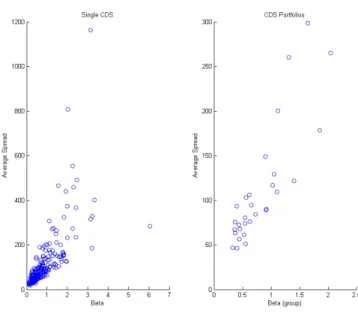
In figure 10 we also represent the scatter plot of the average quoted spread
during the considered period versus theβ estimated from equation (7). We
present the dispersion for both the single CDS and the 30 portfolios. The relationship is strongly positive. This means that the protection against default for companies with a bigger (linear) exposition to systematic credit risk is more expensive. Nevertheless, we cannot directly interpret the CDS spread as a risk premium and therefore we cannot conclude that the a premium for bearing systematic risk exists and is positive.
Indeed, in a world in which agents are risk neutral the CDS spread is just the compensation for the expected loss, where the expectation is computed using the risk-neutral default probabilities. In the real world, agents may use physical default probabilities (in general lower than risk neutral ones) and include a risk premium in the spread they require for bearing default risk or equivalently for unexpected loss, which is neglected by risk neutral agents. In general we don’t know the degree of risk aversion of the agents in the market and therefore from the presented dependence we can only conclude that companies with higher systematic credit risk have a higher risk-neutral expected loss or are characterized by a higher compensation for unexpected loss.
We then move to consider realized returns rather than spreads, and in particular we examine the cross section relationship expressed in equation (8). Graphically, we observe in figure 11 the presence of a positive relationship between systematic risk (β) and returns realized in the period. Nevertheless datapoints seem quite dispersed around the fitted line and the relationship appears quite weak.
Coefficient t-stat γ -0.1847e-03 -4.3801
λ 0.1430e-03 2.4643
Also the F statistic is very high and its p-value is less than 1%. The
cross-section R2 on the 30 groups is equal to 36.32%. The coefficients in the
regression are referred to two-weeks returns. If we annualize them, we get an intercept equal to -48 bps and a slope equal to 37 bps. We can interpret the slope as a risk premium paid to the bearer of systematic credit risk per unit of beta. This premium is only the remuneration for the unexpected loss that a risk averse agent requires.
We can compare our estimate with the results in some of the articles men-tioned in section 2. Liu et al. [2002] estimated a premium equal to 45 basis points per year. However, their estimate is based on the spread between Interest Rate Swaps and Treasury rates at a 10 years maturity. So they consider a longer horizon and only firms in the financial sector. Hull et al. [2005] estimate a premium of 66 basis point for investment grade bonds but all the maturities they are considering are greater than 6 years. Finally a work by Lonstaff et al. [2010] proposes a risk premium equal to about 80 basis points, which is more than twice our estimation. However, this last study is based on secular bond data (almost 150 years). Consequently, we argue that their sample is quite different from ours. For instance, the vast majority of listed companies at the beginning of their sample, and before the crisis of the 1870s, was in the railroad sector while today such sector is almost completely absent from the benchmark indexes.
The estimation of the premia on the CDS rather than on the corporate bonds market arises questions about the presence of a remuneration for the default risk of the counterparty and not only of the reference entity. In this case we can rely on the work by Arora, Gandhi, and Longstaff [2011] in which the presence of a counterparty premium is proved to be statistically significant but almost negligible from the economic point of view. According to the article, both the statistical significance and the economic magnitude increase after the Lehman collapse but they still remain quite small. The reason for this may be the presence of margin requirements and collateralization conventions usually adopted in the market, which should strongly reduce counterparty risk. The presence of a risk premium automatically shows that the theoretical “sufficient diversification” condition given in Jarrow et al. [2005] is actually not verified in the market.
The presence of a credit risk premium can also be justified by the results in section 3, where a considerable correlation between equity and credit market is shown. This fact reduces the diversification opportunities for the investors, who consequently require a premium for investing in the credit market.
In conclusion, the presence of a positive risk premium seems to be justified and its numerical estimation seems quite reasonable compared to other studies, especially when we consider that our estimation period is characterized by the presence of the financial crisis, which lowers the realized returns and therefore the realized risk premia.
5.2.1 A comparison with the Equity Premium
In order to have an idea of the reliability of the estimated premium, we apply the method just described to the computation of the equity risk premium for the same sample of companies in the same period.
In order to reduce the effects produced by the above mentioned measurement error in betas, we use again the grouping approach based on 30 portfolios. We still need an instrumental variable that is correlated to the equity beta but measured independently on it. In analogy with the previous paragraphs, we use the credit beta as instrumental variable and form the portfolios based on it.
The results of the time series estimation are presented in the following table. As before, the point estimate is the average of the single estimations and the t-statistic is based on the cross-sectional standard deviation of the estimated betas.
Coefficient t-stat
α 0.0026 11.7843
β 1.1874 8.7234
The averageR2of the 30 portfolios is in this case 71.79%. The F statistics is always strongly significant.
When we consider the cross section relationship of equation (8), we estimate the following coefficients
Coefficient t-stat
γ 0.0024 5.5992
λ 0.0011 2.8957
Both the coefficients are significant. The cross-section R2on the 30 groups
is equal to 24.46%. If we annualize the estimated coefficients, we get an estimated equity risk premium equal to 2.45% per year.
We can derive some conclusions from the comparison between the credit and equity linear model. First, the fraction of cross-sectional variance explained
by the model is greater in the credit model case, where theR2is more than
36%. This may indicate that the use of the systematic returns as unique risk factor is more appropriate in the credit market than in the equity market or,
equivalently, that the impact of the idiosyncratic component is less important in the credit market, more dependent on systematic factors.
Second, in both cases a significant cross-section intercept is present. This means that the simple linear model is not able to capture the total cross-sectional variability in a complete way. It seems reasonable to conclude that the linear specification is not appropriate or that some other explanatory variable is missing.
Third, we observe that the relatively small credit risk premium comes with a relatively small risk premium on the equity market, at least if compared to other standard studies such as Mehra and Prescott [1985]. This may be a consequence of the sample of firms or of the time period in which the estimations are performed.
6
Some tests of the model
There are many ways to test a model like the proposed one. Here we present some simple tests in the cross-sectional dimension. The main purpose is to verify if systematic credit risk is actually priced and if it is able to explain the cross section of CDS returns.
In particular, if we consider equation (6), the model predicts an interceptγ
statistically equal to zero and a generally positive coefficientλ. The estima-tions for the interceptγ and the coefficient λ, respectively, are presented in the following two tables. Results are referred to grouped data and annualized.
γ Coefficient t-stat 10/2003-7/2007 -0.0006 -0.3306 7/2007-9/2010 -0.0097 -7.9230 10/2003-9/2010 -0.0048 -4.3801 λ Coefficient t-stat 10/2003-7/2007 0.0039 1.7706 7/2007-9/2010 0.0036 2.7594 10/2003-9/2010 0.0037 2.4643
The CDX factor is priced on the entire sample at standard confidence levels. On the pre-crisis period the relationship appears weaker and the factor is priced only at the 90% level, while in the second sub-period the t-statistic is 2.76.
On the other hand, the estimated intercept seems to be insignificant in the pre-crisis period but becomes significantly negative during the crisis and on the entire sample. This means that during periods of stress the model seems
to be too simple and some of the unexplained information is captured by the constant. It is possible that the impact of systematic risk becomes less elementary in those periods, involving non-linear relationships or stronger extreme connections.
6.1 Impact of other factors
We want to verify if the estimated premium actually comes from the remu-neration of systematic non-diversified credit risk or from other sources of risk. One possibility we can probably exclude is liquidity risk. CDS are synthetic instruments, available in theoretically unlimited quantities, which eliminates the exposure to liquidity conditions. Nevertheless we tried to verify the role of some liquidity factor. One issue here is that many commonly used liquidity factors are both liquidity and credit factors. For instance spreads such as the TED or the Libor-OIS spread cannot be considered as pure liquidity indicators. In fact, they incorporate a reward for the credit risk of the financial intermediaries that are operating on the Libor market, which are not risk-free and whose default probability significantly increased during the crisis. In this way the proxy for liquidity risk would include also some components of credit risk, and would reduce the orthogonality between the two risks. On the other hand, an indicator like Pastor-Stambaugh seems difficult to compute on frequencies higher than one month, as in our case. This is because these indicators are in essence regression coefficients, whose estimation on 10 working days only appears unreliable.
We used therefore two bid-ask spreads: the bid-ask of the 30-year on-the-run T-Bond and the bid-ask spread of the 3 months Eurodollar future rate. These quantities can be considered as indicators of the liquidity in the fixed-income market at short and long maturities and do not include any considerable counterparty risk. It turns out that they are both insignificant and not priced and their effect on the estimated premium is in general negligible.
We also add other factors to the statistic characterization of credit returns proposed in equation (4). We added an indicator of economic cycle and other indicators of interest rate conditions. In particular, we take the slope of the term structure of interest rates (10-2 years spread) as indicator of business cycle and the observed zero interest rates at different maturities.
Thus the additional regressors included are
• the changes in the bid-ask spread of the US Eurodollar deposits with maturity 3 months
• the changes in interest rates at all the maturities from 3 months to 10 years
• the change of the difference between 10 and 2 years interest rates (Slope)
• the returns of a broad BBB bond index We therefore consider the regression
ri,t=αi+β1,irCDX,t+β2,iXt+εi,t (10)
whereXt is the generic additional factor used.
As before, we first estimate the time-series regressions for the 30 groups and then the cross-section one including the CDX index and each of the mentioned regressors separately. The increase in theR2for grouped data is only marginal (1-2% on average). The regressors that give the best improvement are long-term interest rate, liquidity indicators and the BBB bond index, although the increase is always less than 5%.
We then look at the significance of the cross-section coefficient estimating the following equation.
ri,t=γ + λ1β1,i+λ2β2,i+ηi (11)
We observe that the new factors are in general not significantly priced. In particular, liquidity factors are statistically insignificant in the cross-section dimension. A strong exception is the BBB bond index, which seems to be statistically priced. This is probably due to the high correlation between the BBB and the CDX index already mentioned above. Another priced factor seems to be the change in the slope of the term structure, but all the considered variables do not significantly affect the cross-section slope coefficients estimated for the CDX index which remains close to 40 bps. Also in this case, the only exception is the BBB bond index, for which a collinearity issue may be present.
Additional Factor λ2 t-stat λ1 t-stat
Eurodollar Bid-Ask 0.0093 0.8967 0.0045 3.8618
T-Bond Bid-Ask -6.005e-5 -0.0969 0.0037 3.8857
Slope 0.0027 3.7350 0.0041 5.2164
6 months zero rate 0.0018 1.2605 0.0045 3.7563
12 months zero rate 0.0019 1.2228 0.0044 3.9023
10 years zero rate -0.0035 -1.7953 0.0040 4.4372
BBB Index returns 0.0171 5.7769 -0.0080 -3.2192
All the t-statistics are corrected for heteroskedasticity in the residuals ac-cording to the Eicher-White method.
7
Systematic risk
One of the goals of this work is to disentangle the systematic component of credit risk from the specific one. There are many possibilities to measure systematic credit risk. The first and most obvious one is just given by the averageR2of equation (4) across single assets or portfolios. Of course, when
the systematic component of risk is high the ability of the market index to explain (on average) the variability of the single CDS will be greater. This means that the behaviour of single credit spreads are strongly driven by common factors and therefore that systematic risk is high.
In the period considered here, we observe an increase of the average R2 of
regression (4) for single CDS and grouped data. We split the time period
into two as in the previous section and verify that the averageR2 increases
from 52.83% in the first period to 57.22% in the second.
Another indication of the increase in systematic risk comes from the principal component analysis of the panel of mark to market variations and residuals from equation (7). As far as returns are concerned, the fraction explained by the first principal component increases from 68.7% in the first period to 78% in the second. If we consider residuals, the increase is more dramatic. The weight of the first component is only 30.12% in the first period and it climbs to 54.73% in the second period. Similar results are obtained if we consider the sum of the first 2 or 3 principal components.
From the first result we can conclude, as before, that the systematic credit risk has increased in the second period. On the other hand, from the second result we conclude that the component of the variance unexplained by the model increases. This means that the simple linear model considered here is able to capture the systematic component of risk in the first non-crisis period but it fails in the second. During the crisis, a considerable portion of the variance remains unexplained by this simple linear model. The presence
of structure in the residuals is also confirmed by the big difference between the weight of the first principal component with respect to the second and the following ones, which does not happen in the first subperiod.
7.1 Variance decomposition
If we observe equation (5) and given the independence properties of ε, we
have that
V (ri,t) =β2iV (rCDX,t) +V (εi,t) (12)
whereV (·) indicates the variance operator. The quantity β2iV (rCDX,t) can be
interpreted as the systematic component of the total variance of asseti, while V (εi,t) is the specific component. The only thing to compute is the evolution
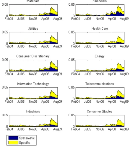
of the variance of the CDX index and of each residual series through time. Given the GARCH structure observed in credit returns described above, we computed the conditional variances of rCDX,t and ˆεt for each of the 10 GICS
sectors according to a GARCH(1,1) model. The results of the decomposition are presented in figure 12.
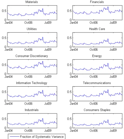
Figure 13 represents the ratio between systematic and total variance in each sector.
We observe a general increase in the systematic component for every sector, which is particularly evident during the crisis period. The financial sector shows the highest fraction of systematic risk compared to all other sectors. This last indicator can also be interpreted as a measure of the fragility of a sector. This interpretation is related to the literature concerning the systematic risk and the frailty factor mentioned in section 2.
The indicator proposed here is much more easily obtained than those discussed above and simply gives a measure of the variability in credit returns of one sector that can be explained by one single observed systematic factor. Of course, if a sector has a very high fraction of its variance explained by one factor, then it seems plausible to consider it as more vulnerable. From our analysis emerges that the financial sector shows the highest degree of fragility. One interesting possibility for future research is to verify the correlation between the latent frailty factor identified by the previously cited articles and the measures here computed.
7.2 Tail dependence
The existence of a systematic component of credit risk originates from the presence of a fraction of risk in the returns of CDS that is not diversifiable. In the previous paragraphs, the presence of non-diversifiable risk has been essentially investigated through the standard Pearson linear correlation, either directly or through the computation of the linear regression coefficients β in equation (7).
It seems worthy to verify the existence of commonality in credit returns beyond the linear Pearson coefficient. In particular, during the last crisis period the existence of extreme dependence in financial markets has become evident. Therefore we studied the dependence between credit returns through the use of copulae.
These functions allow us to model separately the marginal and joint distribu-tions of returns. In particular, a key result in the theory, Sklar’s theorem, relates marginal and joint distributions of a random vector in the following way
H (x1,x2, ...,xn) =C (F1(x1) ,F2(x2) , ...,Fn(xn)) (13)
where
• H (x1,x2, ...,xn) is the joint distribution function computed at points
x1,x2, ...,xn
• C (u1,u2, ...,un) is the copula function, which is a functionC : [0,1]n→
[0,1]
• Fi(xi) is theith marginal distribution function computed at the point
xi.
In our case we use as marginal distribution the empirical CDF combined with a Generalized Pareto distribution for the extreme quantiles. We also assume that the variances of each margin have a GARCH(1, 1) structure, which agrees with the empirical findings of section 3. This quite complicated structure of margins has been successfully applied to the equity market (see e.g. McNeil and Frey [2000] or Nystrom and Skoglund [2002]) and, due to the similarities detected before, we extended it to the credit market. As far as the joint distribution function is concerned, we have to use a copula function that allows for the presence of extreme tail dependence. This measure indicates the comovement between two random variables when extreme events occur, that is when the observed values come from the tails of the distributions. In particular, it describes the limiting fraction of data from one variable exceeding a certain quantile given that the other variable
has exceeded the same quantile. So this quantity can be interpreted as a measure of the “extreme systematic risk” present in the market.
For some copula functions, such as the Gaussian copula, the tail dependence is zero. This means that such copulae show asymptotic independence and no correlation between extreme events. Consequently, we decided to study extreme correlation using two other copulae: Clayton and Gumbel. They both belong to the family of Archimedean copulae and are characterized by the presence of extreme tail dependence. In particular, the Clayton copula shows extreme lower tail dependence (in the left tail) while Gumbel Copula shows extreme upper tail dependence (in the right tail). Our work in this case is quite similar to what Longin and Solnik [2001] applied to the equity market.
We compute the coefficients of upper and lower tail dependence in the pre-crisis and post-pre-crisis period for all the possible pairs of sector return. In this way we obtain a matrix of tail correlation coefficients for all the 10 GICS sectors considered. We then compute the simple average of all the obtained correlation coefficients. We observe a considerable increase in both the lower and upper tail correlation. In particular the left tail coefficient increases from 0.43 to 0.55 (+26.24%) and the right tail coefficient increases from 0.15 to 0.6 (+288.1%). For a comparison, the standard linear Pearson correlation coefficient increases from 0.696 to 0.776 (+11.59%) only. This means that the increase in the non-extreme component of systematic risk is much lower than the increase in the extreme systematic risk for the credit market. The results are summarized in the following table.
10/2003-7/2007 7/2007-9/2010 % Change
Linear Pearson Correlation 0.6955 0.7762 +11.59%
Lower tail dep. coefficient 0.4318 0.5451 +26.24%
Upper tail dep. coefficient 0.1535 0.5958 +288.1%
Table 10: Changes in correlations
7.3 Sector analysis
We now analyze in detail the systematic risk of every sector. We start considering the evolution of the beta coefficient in equation (7) computed for every sector (Table 11). The average returns of the companies in every sector used for the regression are equally weighted.
Sector 10/2003-7/2007 7/2007-9/2010 Materials 1.2111 0.8367 Financials 0.6140 1.3458 Utilities 1.1242 0.5765 Health Care 0.7022 0.4041 Consumer Discretionary 1.3350 1.1267 Energy 1.0795 0.7161 Information Tech. 1.2357 0.7403 Telecomm. 1.7112 0.7951 Industrials 0.6337 0.5749 Consumer Staples 0.5676 0.4270
Table 11: Beta of the sectors
It’s easy to notice a sharp increase in the systematic exposure to systematic risk of the financial sector in the second period, compensated by a decrease in all the other sectors.
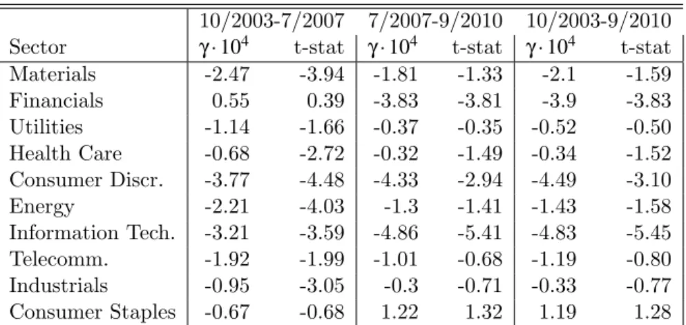
Given the particular evolution of the systematic exposure of the financial sector, we repeated the time series and cross section analysis presented above for the single CDS contracts present in each of the 10 sectors. Cross section coefficientsγ and λ are reported in tables 12 and 13.
10/2003-7/2007 7/2007-9/2010 10/2003-9/2010
Sector γ ·104 t-stat γ ·104 t-stat γ ·104 t-stat
Materials -2.47 -3.94 -1.81 -1.33 -2.1 -1.59 Financials 0.55 0.39 -3.83 -3.81 -3.9 -3.83 Utilities -1.14 -1.66 -0.37 -0.35 -0.52 -0.50 Health Care -0.68 -2.72 -0.32 -1.49 -0.34 -1.52 Consumer Discr. -3.77 -4.48 -4.33 -2.94 -4.49 -3.10 Energy -2.21 -4.03 -1.3 -1.41 -1.43 -1.58 Information Tech. -3.21 -3.59 -4.86 -5.41 -4.83 -5.45 Telecomm. -1.92 -1.99 -1.01 -0.68 -1.19 -0.80 Industrials -0.95 -3.05 -0.3 -0.71 -0.33 -0.77 Consumer Staples -0.67 -0.68 1.22 1.32 1.19 1.28
Table 12: γ of the sectors in the three periods
In this case some sectors include only a small number of companies. This makes the grouping approach not feasible. We therefore implement an analysis based on the single CDS and then correct the standard errors (and consequently the t-stats) according to Shanken [1992].