Large eddy simulation of urban features for Copenhagen metropolitan area

(1)

HAL Id: hal-00327983

https://hal.archives-ouvertes.fr/hal-00327983

Submitted on 2 Nov 2005

HAL is a multi-disciplinary open access

archive for the deposit and dissemination of sci-entific research documents, whether they are pub-lished or not. The documents may come from teaching and research institutions in France or abroad, or from public or private research centers.

L’archive ouverte pluridisciplinaire HAL, est destinée au dépôt et à la diffusion de documents scientifiques de niveau recherche, publiés ou non, émanant des établissements d’enseignement et de recherche français ou étrangers, des laboratoires publics ou privés.

Large eddy simulation of urban features for Copenhagen

metropolitan area

A. Mahura, S. Leroyer, P. Mestayer, I. Calmet, Samuel Dupont, Nathalie

Long, A. Baklanov, C. Petersen, K. Sattler, N. W. Nielsen

To cite this version:

A. Mahura, S. Leroyer, P. Mestayer, I. Calmet, Samuel Dupont, et al.. Large eddy simulation of urban features for Copenhagen metropolitan area. Atmospheric Chemistry and Physics Discussions, European Geosciences Union, 2005, 5 (6), pp.11183-11213. �hal-00327983�

(2)

ACPD

5, 11183–11213, 2005 Large eddy simulation of urban features A. Mahura et al. Title Page Abstract Introduction Conclusions References Tables Figures J I J I Back Close

Full Screen / Esc

Print Version Interactive Discussion

EGU

Atmos. Chem. Phys. Discuss., 5, 11183–11213, 2005 www.atmos-chem-phys.org/acpd/5/11183/

SRef-ID: 1680-7375/acpd/2005-5-11183 European Geosciences Union

Atmospheric Chemistry and Physics Discussions

Large eddy simulation of urban features

for Copenhagen metropolitan area

A. Mahura1,2,3, S. Leroyer1, P. Mestayer1, I. Calmet1, S. Dupont4, N. Long1, A. Baklanov2, C. Petersen2, K. Sattler2, and N. W. Nielsen2

1

Laboratoire de M ´ecanique des Fluides, UMR CNRS 6598, Ecole Centrale de Nantes, ECN, France

2

Danish Meteorological Institute, DMI, Copenhagen, Denmark 3

Institute of Northern Environmental Problems, Kola Science Center, Apatity, Russia 4

EPHYSE, Institut National de la Recherche Agronomique, Bordeaux, France

Received: 26 August 2005 – Accepted: 10 September 2005 – Published: 2 November 2005 Correspondence to: A. Mahura (ama@dmi.dk)

(3)

ACPD

Full Screen / Esc

EGU

Abstract

The large eddy simulations employing the SUBMESO model with the urban soil layer model SM2-U were performed for the model domain covering the Danish Island of Sealand and including the Copenhagen metropolitan area. Monthly and diurnal cycle variability were studied for the net radiation, sensible and storage heat fluxes, surface’s 5

temperatures, and others. These were evaluated for selected urban vs. non urban re-lated types of covers/surfaces and urban districts such as city center, high buildings, industrial, and residential. Results showed strong effects of urban features on tempo-ral and spatial variability. They are useful and applicable for verification of numerical weather prediction models and development of urban canopy parameterizations. 10

1. Introduction

The large eddy simulation (LES) is a good and suitable, although computationally not relatively cheap, method for research and verification of meso-meteorological and nu-merical weather prediction (NWP) models. The LES term was first time introduced by Leonard (1974), and the first successful LES was performed by Deardorff (1970). This 15

term is used for solutions of the full Navier-Stokes equations, where evolution of dif-ferent scales of motion is computed without any turbulence models (Reynolds, 1990). The LES method computes spatial and temporal details of large eddies using simple subgrid scale model for effects of small eddies on the large eddies. A large variety of studies employing LES were performed, especially in engineering and geophysi-20

cal fields, with respect to applications and investigation of the boundary and surface layer structure in non urban and urban areas, turbulent convection, cloudy boundary layers, land-surface interactions, canopies, subgrid-scale studies, ocean mixed layers, etc (see e.g. Galperin and Orszag, 1993).

In urban areas, in contrast with rural areas, the urban boundary layer is more com-25

(4)

ACPD

Full Screen / Esc

EGU

major equation used in many models to evaluate thermodynamical and dynamical pat-terns above the ground surface. In respect with the urban areas it includes the storage, sensible, and latent heat fluxes (plus, anthropogenic heat flux). Note, in these areas, the meteorological network is sparse and measurements do not reflect the charac-teristic meteorological state of the urban terrain (Piringer at al., 2002), i.e. are not 5

representative. Moreover, the fluxes are not directly measured at such stations. The experimental studies (in North American cities, during summer time) (Grimmond and Oke, 1995) on evaluation of local-scale surface heat flux variability showed that, in gen-eral, the fluxes have magnitudes and diurnal behavior similar to rural areas. But within the city itself there are differences between different districts. Moreover, the findings 10

might be not similar (i.e. might be not directly extrapolated to the European cities due to differences in the land-use categories, urban morphology, climatology, etc.). To test it several field campaigns were conducted: 1) BUBBLE in Basle, Switzerland (Rotach et al., 2004); 2) ESCOMPTE in Marseilles, France during June–July 2001 (Mestayer and Coll, 2005); 3) in Birmingham, UK in 1998–2000 (e.g., Piringer and Joffre, 2005). 15

However, such measurements are expensive and cannot be utilized for all cities. Hence, LES can be employed as a numerical substitute or research tool in studies of surface and urban boundary layer development, and its properties and character-istics, etc. Note, the experimental data for the Copenhagen metropolitan area are not available, although these are very important for improvements of the DMI HIigh 20

Resolution Limited Area (HIRLAM) operational NWP model performance, especially on finer resolution scales. In our study, therefore, we used LES (done by SUBMESO atmospheric model coupled with Soil Model for Sub-Meso scales Urbanized version (SM2-U) model – developed at ECN) to investigate the monthly and diurnal variability of the net radiative, sensible, and storage heat fluxes and temperatures for different 25

types of covers/surfaces and urban districts. It was done on example of the simulations in the model domain covering the Danish Island of Sealand and surroundings (includ-ing the Copenhagen metropolitan area). The results of this analysis will be used further for evaluation of performance of the DMI-HIRLAM NWP model urbanized with SM2-U

(5)

ACPD

Full Screen / Esc

EGU

for the same model domain.

2. Methodology

2.1. Land use classification, urban districts and its characteristics

High quality land-use classification (LUC) data is a crucial input in NWP modeling. In our study, as input, the CORINE dataset (based on 40 different types of surfaces over 5

Europe, resolution of 250 m, version of year 2000; CORINE, 2000) providing a bet-ter representation of orography and identification of urban surface features was used to prepare LUC in the model domain area. The classification of the CORINE dataset was done on the selected domain located between 10.44–13.41◦E and 54.81–56.50◦N (118×124 grid points) with a resolution of 1.4×1.4 km. For each grid cell, the clas-10

sification is represented by 7 types of covers/surfaces: bare soil without vegetation (BARE); bare soil located between sparse vegetation elements (NAT); vegetation over bare soil (VEGN); vegetation over paved surfaces (e.g., trees on the road side: VEGA), paved surfaces located between the sparse vegetation elements (ART), building/roofs (BAT), and water surfaces (EAU) (see also Appendix A). Note, classification followed 15

the “mosaic” approach, where each cell may contain up to 7 different types of surfaces. Further, the cells, where contribution of BAT-type into cell was more than 75%, were assigned to the city center and high buildings districts (CC/HBD); 50–75% – industrial commercial district (ICD), and less than 50% – residential district (RD). The other cells, where BAT-type was not presented at all, were considered as rural or non urban areas. 20

The cells where the fraction of EAU-type was equal to 1 (65.93% from total number of cells) were considered as the water areas. The results of the land use classification for the entire domain and its statistics are summarized in Table 1, and shown in Fig. 1 on example of the Island of Sealand, located in the center of model domain.

Analysis of the Copenhagen city aerial photos showed that two types of districts – 25

(6)

characteris-ACPD

Full Screen / Esc

EGU

tics, since there is no clearly independent city center type of the district (with specific properties) such as in the North American cities. Similarly to analysis of the city of Marseille, France (where the BDTopo database and software DFMap were employed to extract morphology, Long and Kergomard, 20041) the selected aspect ratios (H/W – height vs. width) are 1.78, 0.9, and 1.125 for CC/HBD, ICD, and RD, respectively. 5

The average heights of buildings are 15.8, 10.7, and 7.3 m; and the average surfaces – 1500, 1223.6, and 263.3 m2– for CC/HBD, ICD, and RD, respectively. As the artificial and building roof surfaces were assumed made of the asphalt and slite with tile (sheet metal – for ICD) were selected. Note that to obtain such characteristics as well as to improve quality and resolution of the land use and urban subclasses the classifica-10

tion of other databases can be used, e.g. Areal Informations Systemets (resolution of 25 m); and building resolved GIS databases of urban structures (BlomInfo A/S).

Moreover, based on the CORINE data it was found also that the ART and VEGA types of surfaces were less represented (i.e. ≈2%) in the domain as it might be expected. Therefore, the re-distribution between fractions of 7 surface types was 15

done. At first (MapInfo software was employed) estimates of fractions of classes were performed based on analysis of the aerial photos for the typical urban sub-classes of the Copenhagen metropolitan area. Then, the following formulations for cells of: 1) CC/HBD: bat_new=0.8·bat_old, art_new=art_old+0.2·bat_old, bare_new=0.5·bare_old, vegn_new=vegn_old+0.5·bare_old; 2) ICD: bat_new=0.4·bat_old and art_new=art_old+0.6·bat_old; 20

3) RD: bare_new=0.5·bare_old and art_new=art_old+0.5·bare_old – were applied for re-calculations. This procedure modified 154, 128, and 291 (i.e. in total 573) cells for CC/HBD, ICD, and RD districts, respectively. The significant changes of re-classification occurred with the increase of ART average from 0.15 to 1.11, and de-crease of BAT average from 3.17 to 2.59%. The BAT maximum also dede-creased from 25

100 to 80%.

1

Long, N. and Kergomard, C.: Indicateurs morphologiques du tissu urbain pour des appli-cations climatologiques, Revue Internationale de G ´eomatique, in review, 2004.

(7)

ACPD

Full Screen / Esc

EGU

2.2. Atmospheric model SUBMESO urbanized SM2-U

The atmospheric model SUBMESO is a compressible non hydrostatic model devel-oped at the Ecole Centrale de Nantes, derived from the Advanced Regional Predic-tion System Version 3 (ARPS; Xue et al., 1995) model. Navier-Stokes equaPredic-tions are solved employing large eddy simulation method (Anquetin et al., 1999). The subgrid-5

scale fluxes are modeled by solving an equation for the turbulent kinetic energy. It allows simulating atmospheric flows with a range of mesh resolution from a few meters to several kilometers. The equations are written in the ‘terrain-following’ coordinate system. An option for stretching grid vertically is available while the mesh is homoge-neous in the horizontal direction. The solution is advanced in time using a time-splitting 10

method. The heat, moisture and momentum fluxes based on the Monin-Obukhov Sim-ilarity Theory are used as boundary condition in the first cell layer at the ground, to model canopy influence on the boundary layer flow.

SM2-U is the urban extension of the force-restore model of Noilhan and Planton (1989). It is composed with 3 soil layers and a canopy layer. In each computational 15

cell at the ground, 7 types of covers/surfaces (see Sect. 2.1) are defined by their char-acteristics and surface density. The horizontal exchanges inside the urban canopy are not considered except radiation reflections and water runoff from saturated surfaces. Surface temperature and humidity of the ground surface types are obtained from the force-restore equations and exchanges with the soil layers. For buildings and water 20

surfaces temperature evolution, a simple conduction equation is used, without force-restore process but excluding exchange through two layers of materials. Important processes like radiative trapping inside the street canyon are parameterized by an ef-fective albedo of the street. Energy and water budgets are performed for each type of surface in order to deduce the heat and moisture fluxes to be set at the interface 25

between canopy and atmosphere. The surface dynamical influence is represented through roughness lengths and displacement heights. The detailed description of the

(8)

ACPD

Full Screen / Esc

EGU

model and its validation results are given by Dupont et al. (2004, 2005a2, b3). A modi-fied version of SM2-U for the FUMAPEX meso-meteorological models is described and tested in Baklanov et al. (2005).

2.3. Input meteorological and surface data, and model setup

To simulate the diurnal cycles on monthly basis employing the SUBMESO model, the 5

input data (meteorological and surface related) were initially prepared for the selected model domain. For each month, a set of characteristics was extracted from the cli-mate generation files produced for the DMI-HIRLAM model system as well as from climatological data for the city of Copenhagen and other Danish sites of the Island of Sealand.

10

The surface oriented data, in addition to mentioned ones in the land use classifi-cation, included also the types of soil, vegetation above natural and artificial surfaces, water, buildings and artificial surfaces, and a set of water content related characteristics in different soil layers, etc.

The meteorological oriented data included the air temperature, direction and velocity 15

components for wind, relative humidity, surface and sea surface temperatures, salinity, soil and deep soil water contents, pressure, roughness. Also the leaf area index was assigned on a monthly basis. Moreover, the wind characteristics, temperature, and humidity values at 925 mb level were also accounted.

In our study, the SUBMESO model with SM2-U module was run in a climatological 20

mode (12 times in total) i.e. with monthly typical averaged meteorological variables in the selected model domain. For each month, first, the relative humidity, air

temper-2

Dupont, S., Guilloteau, E., Mestayer, P. G., Berthier, E., and Andrieu, H.: Parameterization of the Urban Water Budget by Using the SM2-U Model, J. Appl. Meteorol., in review, 2005a.

3

Dupont, S., Calmet, I., Mestayer, P. G., and Leroyer, S.: Parameterization of the Urban Energy Budget with the SM2-U Model for the Urban Boundary Layer Simulation, Boundary Layer Meteorology, in review, 2005b.

(9)

ACPD

Full Screen / Esc

EGU

ature, wind direction and its velocity components at two levels – surface and 925 mb – were used to recover the typical vertical profiles of the humidity, temperature, and wind characteristics within the boundary layer and free troposphere. It was done for initialization step at 00:00 UTC, where the atmosphere was considered as hydrostatic and stably stratified. The land surface and deep soil temperatures were also initialized 5

at 00:00 UTC. Moreover, the properties of the type of soil, roof, and artificial surface in each cell of model domain were used, with incorporation of monthly values of soil and deep soil water contents, leaf area index, sea surface temperature, and salinity. The diurnal cycle of the solar radiation and precipitation rate were included.

The first vertical level was at 40 m, and the grid was extended up to 9 km with the 10

Rayleigh layer imposed between 6–9 km. Zero gradient condition was set up for the lateral boundaries. The time steps for integration and for the soil model were imposed at 1 s.

2.4. Simulated output data and their treatment

All SUBMESO simulated outputs were saved every 30 min (and/or 1 h) intervals. The 15

entire size of data output (for each month) is equal to 1.2 Gb in compressed format. The CPU time used (run on 1 processor) is equal up to 50 h for the DMI NEC-SX6 supercomputer; although the real time usage, depending on the current loading of the NWP operational machine, is higher.

For analysis, the output was re-arranged in time series. Each record in series con-20

tained information about month, UTC and local time, numbers (or identifications) of grid points along latitude and longitude, distances in meters along latitude and longi-tude starting from the south-west corner (10.44◦E and 54.81◦N) of the model domain, category of the grid cell in relation with urbanized features, and a set of calculated variables for 7 types of surfaces.

25

In our study, among variables, selected and re-recorded further for analysis, were the following: net radiation, sensible, and storage fluxes [in W/m2]; soil and surfaces’ temperatures, air temperature [in K], water vapor specific humidity [in kg/kg], and wind

(10)

ACPD

Full Screen / Esc

EGU

velocity [in m/s]. These were selected because of further comparison and evaluation of performance of the DMI-HIRLAM NWP model urbanized with SM2-U for the same model domain. The required storage for the mentioned above variables is equal to 0.6 Gb (non archived format) per one month. It should be noted, that a set of other simulated by SUBMESO variables (in total more than 50) is available. These, for ex-5

ample, include also derived characteristics such as dynamical velocity, turbulent kinetic energy, dissipation, etc.

The category of the grid cell was defined following mentioned results of LUC. In this study, three types of districts (i.e. CC/HBD, ICD, and RD) were assigned to each grid cell, where these were represented in the model domain. In addition, for simplifica-10

tion and comparative purposes, the grid cells, where the BAT type of surface was not presented at all, were assign to cells representing non urban areas. The cells oc-cupied only by EAU were assigned to additional category and further excluded from analysis. Moreover, most of the simulated variables were treated with respect to the “land” related surfaces, except EAU. The types such as BAT, ART, and VEGA were also 15

distinguished as more related to the urbanized areas compared with others.

In this study, evaluation of simulated variables (in the next section) included the month-to-month variability, diurnal cycle on the annual (entire dataset) and monthly scales, and analyses for 7 types of selected surfaces as well as for different districts (urbanized vs. non urban areas). The districts such as CC/HBD, ICD, and RD were 20

represented in total by 41, 110, and 1058 grid cells of the model domain, respectively. Hence, statistics given for the BAT type of surface will be more biased toward the resi-dential district patterns. Note, in all further figures the diurnal cycle is presented on the UTC scale, but the local time will be 1 h of difference for the selected model domain. Moreover, the use of the “mosaic” approach (i.e. when in each grid cell the fractions 25

of different surfaces/covers were taken into account) allowed to represent into more details the behavior of urban districts on diurnal and monthly scales.

(11)

ACPD

Full Screen / Esc

EGU

3. Results and discussions

3.1. Net radiative fluxes

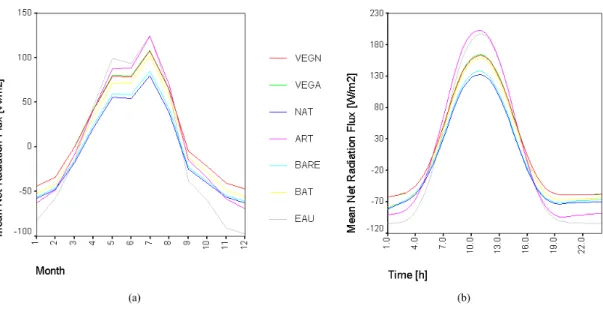
The monthly variability of the mean net radiation fluxes (NRF) for 7 types of surfaces is shown in Fig. 2a. As seen, during September–March, the NRF for all types of sur-faces is negative, although for VEGA starting in March it became positive. Flux is the 5

lowest for EAU during September–February and for ART during November–February – with minima of −97 and −69 W/m2, respectively, both observed in December. Dur-ing March–August, in general flux is lower for NAT compared with other surfaces. The highest NRFs for all types of surfaces are observed in July. Among these types the highest mean value of 125 W/m2is for both the EAU and ART surfaces; and the lowest 10

values of 85 and 80 W/m2are for the BARE and NAT surfaces, respectively. Note, dur-ing July, in some cells NRFs up to 567 and 523 W/m2 were observed for the BAT and ART types, correspondingly.

The diurnal variability of the mean NRFs is shown in Fig. 2b. As seen, the largest values of fluxes for all types of surfaces are observed during noon time, with the highest 15

for the EAU and ART surfaces, followed by VEGA, VEGN and BAT, and concluded by NAT. During 17:00–06:00 h, the flux is the lowest for EAU compared with other types.

Detailed analysis of diurnal variability on a monthly basis for the urban cells with representation of the CC/HBD and ICD districts showed the following. For the CC/HBD cells, on a diurnal cycle, the NRF is always negative during December–January. Be-20

ginning of February it became positive between 09-13 hours and reached a maximum of 33 W/m2 at 11:00 h. Further, the duration of positive NRF is increased gradually – between 05:00–17:00 h – until July, with a maximum of 382 W/m2 at 11:00 h and a minimum of −67 W/m2at 20:00 h. The monthly variability underlined that during April– August the daily mean flux is positive, and it is negative in all other months. The daily 25

mean NRF is the highest (104 W/m2) in July and the lowest (−47 W/m2) – in December. For the ICD cells, on a diurnal cycle, there are always periods showing positive NRFs. The duration of such periods is the shortest (08:00–14:00 h) during December–

(12)

ACPD

Full Screen / Esc

EGU

January. It gradually increased during spring, reaching a maximum of duration in June (03:00–19:00 h), and then decreased until December. The maximum value of flux is 548 W/m2 and it is observed in July at 11:00 h. The minimum of −23 W/m2is charac-teristic for the late evening and night hours during July–August. The monthly variability showed that throughout the year, except December–January, the daily mean NRF is 5

always positive, but with significantly larger standard deviations – 27(11) W/m2in sum-mer (winter) months – compared with up to 2 W/m2for CC/HBD. Note, the daily mean NRF is the highest (200 W/m2) in July and the lowest (−7 W/m2) – in December. 3.2. Surface temperatures

The monthly variability of the mean soil and surfaces’ temperatures is shown in Fig. 3a. 10

As seen, throughout the year the mean temperature is always positive for ART and EAU compared with other surfaces. The highest temperatures are characteristic for the ART and BAT types in July reaching up to 22 and 20.3◦C, respectively (with maxima of 31.3 and 35.4◦C in some cells of domain containing these types). But in August, the soil and EAU has own highest (on an annual scale) mean temperatures of 15.6 and 18.7◦C, 15

respectively. During December–February, for the VEGA, VEGN, BARE and BAT types (November – also for VEGA and VEGN), the temperature is negative, although in other months it is always positive with maxima in July. During September–March, it is the lowest for both VEGN and VEGA among other land types of surfaces. In January, in some cells it reached even −7.6◦C, although on average it was −4.7◦C during this 20

month. Note, in some cells of domain, for these two types the negative temperatures can be observed starting already in August and extended farther into April. For BAT, such situation is observed during November–April.

The diurnal variability of the mean surface temperatures is shown in Fig. 3b. Note, the temperature variability of the soil and water surface is significantly smaller com-25

pared with the “land” types of surfaces and hence, these were omitted from figure. The largest difference is seen between VEGA and VEGN vs. ART reaching of more than 5◦C during 16:00–04:00 h (maximum of 8◦C at 18:00 h). Moreover, the daily maximum

(13)

ACPD

Full Screen / Esc

EGU

of the ART’s temperature is comparable with VEGA, VEGN and BAT, although occurred 2 h later. Note, that also 1 h later occurred a daily maxima (smaller of magnitude) for the NAT and BARE types. The minima are characteristic for the VEGA and VEGN types during the late evening and night hours.

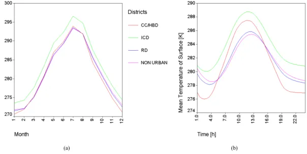
The monthly and diurnal cycle variability of the mean temperature of the surface 5

(calculated taking into account influence from all 7 possible types of surfaces presented in grid cells) for selected types of districts is shown in Fig. 4. Detailed analysis of diurnal variability on a monthly basis for the urban cells showed the following.

For the CC/HBD cells, on a diurnal cycle, the temperature is always positive (i.e. above 0◦C) during May–October. Beginning of January it became positive (but 10

only less than 1◦C) between 11–12 h. Further, the duration of positive temperatures is increased gradually until April, as well as it gradually decreased during November– December. The daily maximum of up to 30◦C can be observed in July in the middle of the day, and a minimum of −6◦C in January in the late evening hours.

For the ICD cells, on a diurnal cycle, the positive temperatures are dominant dur-15

ing all months, except January–February. Moreover, they also positive, at least, during 08:00–16:00 h for these two months. Similarly to the CC/HBD cells, the daily maximum (33◦C) can be observed in July in the middle of the day, and a minimum (−0.4◦C) in Jan-uary in the late evening hours. Moreover, for CC/HBD, the monthly variability showed that throughout the year, except December–February, the daily mean temperature is 20

always positive. Note, for ICD – it is always positive.

3.3. Air temperature, water vapor specific humidity, and wind velocity

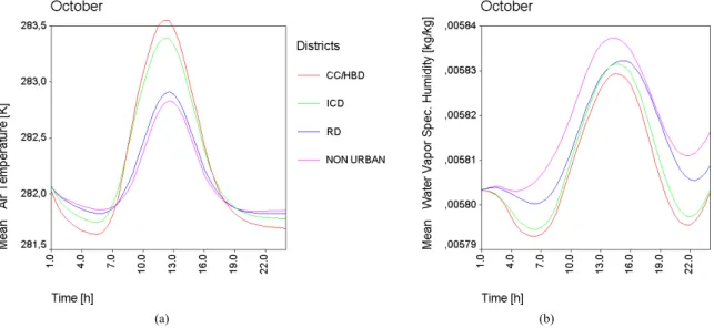
For the urban cells of model domain, an additional analyses of diurnal cycle for the simulated air temperature, water vapor specific humidity, and wind velocity were per-formed (for the first two variables an example is shown for October in Fig. 5). As seen 25

in Fig. 5a, during this month the maxima of the mean air temperature in CC/HBD and ICD occurred at noon and one hour earlier compared with the RD and non urban ar-eas. Moreover, on a diurnal cycle, the maximum difference between air temperatures

(14)

ACPD

Full Screen / Esc

EGU

in mentioned areas was less than 0.8◦C. During 18:00–07:00 h, the air temperature in the CC/HBD cells was always slightly lower compared with all other cells, although be-tween 09:00–16:00 it was higher. For non urban areas, the air temperature was always slightly higher and lower during periods of 20:00–06:00 h and 08:00–18:00 h, respec-tively. These general patterns remained similar on a month-to-month scale, although 5

the maximum differences and amplitudes as well as beginning and duration of periods with higher/lower temperatures for considered districts depended on analyzed months. The October diurnal cycle of the mean water vapor specific humidity is shown in Fig. 5b. As seen, the CC/HBD cells had the lowest values compared with all other cells. In opposite, for the non urban areas, the values are the highest. The maxima 10

for these as well as the ICD cells is observed between 14:00–15:00 h, although for RD it shifted forward by one hour. The minima are characteristic for the early morning and the late evening hours. Although note, that the shown pattern is not similar on the month-to-month scale and occurrence of maxima and minima can be significantly shifted on a diurnal cycle depending on a water availability.

15

On a diurnal cycle, the differences in mean wind velocities between the CC/HBD, ICD, and RD districts are negligible (of less than 0.3 m/s, with the slightly higher veloc-ities within the RD cells compared with two others). Note, month-to-month variability showed a similar pattern.

3.4. Sensible heat flux 20

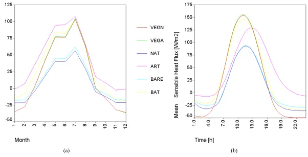
The monthly variability of the mean sensible heat fluxes (SHF) for different land surface types is shown in Fig. 6a. As seen, throughout the year this flux is positive for all types during March–September, except NAT and BARE (these two remained still negative in March and September). The ART type has the longest duration (starting in February and ending in October) of positive SHF with a maximum of 107 W/m2in July. The VEGN 25

and VEGA types have the lowest SHF values of less than −25 W/m2corresponding to the November–February period. The highest difference (of up to 50 W/m2) between SHFs in urban vs. non urban related is observed during late spring – summer months.

(15)

ACPD

Full Screen / Esc

EGU

The diurnal variability of the mean SHF is shown in Fig. 6b. The late evening – night hours are characterized by negative fluxes for all types of surfaces. But for “urban related surfaces” such as BAT, ART, and VEGA it became positive earlier compared with “non urban related surfaces” (i.e. over types studied) by up 1 h. Moreover, for ART it will remain positive for significantly longer time (up to 21:00 h) compared with all 5

others. The daily maximum of ART SHF (129 W/m2) occurred around 13:00 h, i.e. 1– 1.5 h later than for other types. The highest values of 154 W/m2 are characteristic for VEGA and VEGN, followed by BAT with 147 W/m2, and the lowest (93 W/m2) are for the NAT and BARE types.

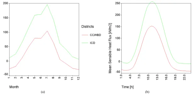
Note, the monthly and diurnal cycle variability for districts is shown in Fig. 7 (resi-10

dential district and non-urban areas were omitted because they showed very similar to HBD results).

Detailed analysis of diurnal variability on a monthly basis for the urban cells showed that for the CC/HBD cells, the mean SHF is always negative only in December reaching up to −36 W/m2 during late evening hours (and a daily mean of −29 W/m2). Note, 15

the daily mean is negative during October–February. Starting of January it became positive at 11:00–12:00 h, and duration of positive fluxes’ occurrence increased until July (05:00–17:00 h), and then gradually decreased. In July, the maximum of more than 350 W/m2 during 10:00–12:00 h is observed (note, in some such cells flux might be up to 402 W/m2).

20

For the ICD cells, on a diurnal cycle, the shortest duration of positive SHF occurrence (08:00–15:00 h) is observed during December–January, while the longest is during May–July (04:00–19:00 h). Note, both the highest (533 W/m2) and lowest (−15 W/m2) values of flux are characteristic at noon and night time in July, respectively (note, in some such cells flux might be up to 638 W/m2). The daily mean is always positive 25

ranging from 6 to 196 W/m2 (December vs. July) with standard deviations of 10 and 27 W/m2, respectively, which are larger by order of magnitude compared with CC/HBD.

(16)

ACPD

Full Screen / Esc

EGU

3.5. Storage heat flux

The monthly variability of the mean storage heat flux (STHF) for land types of surfaces is shown in Fig. 8a. As seen, throughout the year the mean STHF is mostly negative. During July–August it is positive for all types of surfaces, except BAT. Starting of April it became also positive for the BARE and NAT types. The lowest fluxes are for the ART 5

type during winter months, reaching of −68 W/m2 in December. The highest fluxes of 23 W/m2are for both the BARE and NAT types in July (in some grid cells these can be more than 350 W/m2). Note, the lowest amplitude is characteristic for the VEGA and VEGN types compared with others.

The diurnal variability (based on the annual dataset) of the mean STHFs is shown 10

in Fig. 8b. As seen, it became positive during 4.5–13 h for both VEGA and VEGN types reaching maxima of 12.5 W/m2 at 09:00 h. With a shift of one hour (from 5.5 h) it became also above zero for the NAT and BARE types with maxima at the same time as the former two. The highest amplitude of the flux is characteristic for the ART type. ART has a maximum of 107 W/m2 at 9.5 h and a minimum of −114 W/m2 at 18:00 h. 15

In general, for all types, the storage heat fluxes were negative during the midday-night time hours.

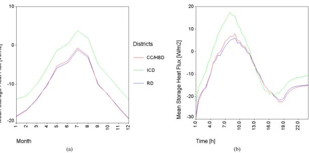
The monthly and diurnal cycle variability for districts is shown in Fig. 9 (non-urban was omitted because it showed patterns very similar to residential district results). De-tailed analysis of diurnal variability on a monthly basis for the urbanized cells showed 20

the following.

For the CC/HBD cells, on a diurnal cycle, STHF is always negative during December–January reaching up to −33 W/m2at night time. First time it became pos-itive in February between 8.5–9 h, then it gradually increased its duration until July (3.5–15 h). During this month it reached a maximum of 22.4 W/m2 at 09:00 h (note, 25

in some such cells flux might be up to 47 W/m2). Further, it gradually decreased until November with a daily maximum of 6.5 W/m2.

(17)

ACPD

Full Screen / Esc

EGU

reaching up to −29 W/m2 at night time. First time it became positive in January at 09:00 h, then it gradually increased its duration until June (03:00–14:00 h). During this month it reached a maximum of 33.6 W/m2 at 08:00 h (in some such cells flux might be up to 54 W/m2). Note, the highest flux of 38.3 W/m2 (8.5 h) is characteristic for July, and in some cells it might be up to 76.6 W/m2. Further, flux gradually decreased 5

until November with a daily maximum of 6.5 W/m2. The RD cells, on a diurnal cycle, showed a similar pattern as the ICD cells, although it is lightly different. First, flux is always negative during December–February (reaching up to −32 W/m2in December at night time) and it became first time positive in March between 07:00–11:00 h. Second, it has the longest duration of positive values in July which begun one hourly earlier (at 10

03:00 h) than for ICD. Moreover, the maximum observed at 9 h is only 21.1 W/m2, but in some RD cells it can be up to 122 W/m2. Similarly, flux gradually decreased also until November with a daily maximum of 6.2 W/m2.

Note, for both the CC/HBD and RD, the STHF’s standard deviations of up to 1 vs. 4 W/m2 are characteristic for the fall-spring vs. summer months, respectively; al-15

though for the ICD cells, these are twice larger.

4. Conclusions

In our study, the large eddy simulations employing the SUBMESO model coupled with SM2-U model were done on the monthly basis for the model domain covering the Danish Island of Sealand and surroundings (including the Copenhagen metropolitan 20

area). Analysis of monthly and diurnal variability of the surface temperatures and fluxes (other simulated and derived variables is also available) was performed for different types of surfaces/covers and districts of urbanized areas.

Detailed analyses showed large monthly and diurnal cycle variability between di ffer-ent types of surfaces, and first of all, for urban related (vegetation over paved surfaces, 25

e.g., trees on the road side (VEGA), paved surfaces located between the sparse vege-tation elements (ART), and building/roofs (BAT) surfaces) vs. non urban related types

(18)

ACPD

Full Screen / Esc

EGU

of surfaces showed the following. For VEGA, ART, and BAT surfaces, the mean net ra-diation flux became positive during April–August (for VEGA starting in March) with the highest (125 W/m2) for ART in July at noon time. The highest mean surface tempera-tures – 22 and 20.3◦C – are characteristic for ART and BAT in July, respectively. The negative temperatures for VEGA can be observed starting already in August, and also 5

for BAT – in November. The positive mean sensible heat flux is characteristic for ART during February–October with a maximum of 107 W/m2in July. The highest difference between fluxes of urban vs. non urban surfaces is observed during late spring-summer months. The mean storage heat flux is the lowest for ART during winter months, and moreover, VEGA has the lowest amplitude compared with other types.

10

For the city center/high building district, the mean daily net radiation flux is positive during April–August. On a diurnal cycle, both the longest duration of positive fluxes (05:00–17:00 h) and a maximum of 382 W/m2 (at 11:00 h) are observed in July. The mean daily sensible heat flux is positive during March–September. On a diurnal cy-cle, both the longest duration of positive fluxes (05:00–17:00 h) and a maximum of 15

350 W/m2(at 11:00 h) are observed in July. The mean storage heat flux is always neg-ative during December–January. On a diurnal cycle, both the longest duration of posi-tive fluxes (3.5–15 h) and a maximum of 22.4 W/m2(at 09:00 h) are typical in July. On a diurnal cycle, the mean surface temperature is always positive during May–October with a maximum of up to 30◦C (July) and minimum of −6◦C (December).

20

For the industrial commercial district, the mean daily net radiation flux is positive during February–November. On a diurnal cycle, the longest duration of positive fluxes (03:00–19:00 h) is observed in June, and a maximum of 548 W/m2 (at 11:00 h) – in July. The mean daily sensible heat flux is always positive throughout the year. On a diurnal cycle, the longest duration of positive fluxes (04:00–19:00 h) is observed during 25

May–July, and a maximum of 533 W/m2 (at 11:00 h) – in July. The mean storage heat flux is always negative only in December. On a diurnal cycle, the longest duration of positive fluxes (03:00–14:00 h) is typical in June, and a maximum of 38.3 W/m2 (at 8.5 h) – in July. On a diurnal cycle, the positive mean surface temperature is dominant

(19)

ACPD

Full Screen / Esc

EGU

throughout the year, except January–February, with a maximum of up to 33◦C (July) and minimum of −0.4◦C (December).

For wind velocities, differences between urban district types were small (of less than 0.3 m/s), although for urban vs. non urban areas these might be larger in individual cells. For air temperature and water vapor mixing ratio, differences are seen in monthly 5

amplitudes, beginning and duration of high/low periods, shifts in occurrence of daily maxima/minima.

The results of this study are useful and applicable for investigation of temporal and spatial variability of various meteorological and derived variables over urbanized ar-eas; for improvements in the land use classification and climate generation properties, 10

distinguishing and selection of types of urban districts and their properties; testing and verification of NWP models performance over high resolution model domains, and es-pecially over the urbanized areas, etc.

(20)

ACPD

Full Screen / Esc

EGU

Appendix A

Abbreviations in Description/Comment text and figures

BARE Bare soil without vegetation

NAT Bare soil located between sparse vegetation elements VEGN Vegetation over bare soil

VEGA Vegetation over paved surfaces (e.g., trees on the road side) ART Paved surfaces located between the sparse vegetation elements

BAT building/roofs

EAU Water surfaces

CC/HBD City center / high buildings district ICD Industrial commercial district

RD Residential district

Acknowledgements. The authors are grateful to L. Laursen, T. Penelon, U. Korsholm for

col-laboration, discussions and constructive comments. The computer facilities at DMI and ECN have been used extensively in the study. The authors are grateful to the HIRLAM group, Data

5

Processing Department, Climate Research group at DMI for the collaboration, computer assis-tance, and advice. Financial support of this study included the grants of the EU FUMAPEX and HIRLAM projects.

References

Anquetin, S., Guilbaud, C., and Chollet, J.-P.: Thermal Valley Inversion Impact on the

Disper-10

sion of a Passive Pollutant in a Complex Mountainous Area, Atmos. Environ., 33, 3953–3959, 1999.

Baklanov, A., Mestayer, P., Clappier, A., Zilitinkevich, S., Joffre, S., Mahura, A., and Nielsen, N.: On the parameterisation of the urban atmospheric sublayer in meteorological models, Atmos. Chem. Phys. Discuss., accepted, 2005.

(21)

ACPD

Full Screen / Esc

EGU

CORINE: CORINE Land Cover Dataset 2000, European Environmental Agency, http://

dataservice.eea.eu.int/dataservice/, 2000.

Deardorff, J. W.: A Numerical Study of Three-Dimensional Turbulent Channel Flow at Large Reynolds Number, J. Fluid Mech., 41, 453–480, 1970.

Dupont, S., Otte, T. L., and Ching, J. K. S.: Simulation of meteorological fields within and

5

above urban and rural canopies with a mesoscale model (MM5), Bound.-Layer Meteorol., 113, 111–158, 2004.

Galperin, B. and Orszag, S. A. (Eds.): Large Eddy Simulation of Complex Engineering and Geophysical Flows, Cambrige University Press, 600 p., 1993.

Grimmond, C. S. B. and Oke, T. R.: Comparison of heat fluxes from summertime observations

10

in the suburbs of four North American cities, J. Appl. Meteorol., 34, 873–889, 1995.

Leonard, A.: Energy Cascade in Large Eddy Simulations of Turbulent Fluid Flows, Adv. Geo-phys., 18A, 237–248, 1974.

Mestayer, P. and Coll, I.: The Urban Boundary Layer Field Experiment over Marseille UBL/CLU-Escompte: Experimental set-up and First Results, Bound.-Layer Meteorol., 114, 315–365,

15

2005.

Noilhan, J. and Planton, S.: A simple parametrization of land surface processes for meteoro-logical models, Mon. Wea. Rev., 117, 536–549, 1989.

Piringer, M., Grimmond, C. S. B., Joffre, S. M., Mestayer, P., Middleton, D. R., Rotach, M. W.,

Baklanov, A., De Ridder, K., Ferreira, J., Guilloteau, E., Karppinen, A., Martilli, A., Masson,

20

V., and Tombrou, M.: Investigating the Surface Energy Balance in Urban Areas – Recent Advances and Future Needs, Water, Air and Soil Poll.: Focus, 2, 1–16, 2002.

Piringer, M. and Joffre, S.: The urban surface energy budget and mixing height in European

cities: Data, models and challenges for urban meteorology and air quality, edited by: Bak-lanov, A., Burzynski, J., Christen, A., Deserti, M., De Ridder, K., Emeis, S., Joffre, S.,

Karp-25

pinen, A., Mestayer, P., Middleton, D., Piringer, M., and Tombrou, M., Final Report of WG2 COST Action 715, 194 p., 2005.

Reynolds, W. C.: The Potential and Limitations of Direct and Large Eddy Simulations, in: Whither Turbulence? Turbulence at the Crossroads, edited by: Lumney, J. L., pp. 313–343, Springer-Verlag, 1990.

30

Rotach, M. W., Vogt, R., Bernhofer, C., Batchvarova, E., Christen, A., Clappier, A., Feddersen, B., Gryning, S.-E., Martucci, G., Mayer, H., Mitev, V., Oke, T. R., Parlow, E., Richner, H., Roth, M., Roulet, Y. A., Ruffieux, D., Salmond, J., Schatzmann, M., and Voogt, J.: BUBBLE

(22)

ACPD

Full Screen / Esc

EGU

– a Major Effort in Urban Boundary Layer Meteorology, Theor. Appl. Climatol., 81, 231–261, 2004.

Xue, M., Droegemeier, K. K., Wong, V., Shapiro, A., and Brewster, K.: Advanced Regional Prediction System ARPS User’s Guide. Version 4.0, Center for Analysis and Prediction of Storms, University of Oklahoma, 380 p., 1995.

(23)

ACPD

Full Screen / Esc

EGU

Table 1. Distribution of surface types and its characteristics (in %) in the model domain based

on classification of the CORINE dataset.

Characteristic

Surface type Max Avg. StD PTS DTS

VEGN 100 4.03 13.30 12.74 2.74 (401) VEGA 79 0.29 2.89 1.48 0.08 (12) NAT 100 3.25 10.95 12.07 1.83 (268) ART 100 0.15 2.65 0.54 0.12 (18) BARE 100 23.48 37.12 29.78 21.79 (3189) BAT 100 3.17 12.70 9.54 2.25 (329) EAU 100 65.62 45.67 75.49 70.74 (8279)

PTS (presented type of surface) – percentage of cells from total number of cells in domain where, at least, a fraction of surface type is presented.

DTS (dominated type of surface) – percentage of cells from total number of cells in domain where a fraction of selected surface type is the highest compared with other types; values given in brackets are number of cells with this type in the model domain.

(24)

ACPD

Full Screen / Esc

EGU

a) b)

Fig. 1. Example of the land-use classification of the CORINE dataset for the Island of Sealand,

Denmark: (a) presented type of the bat surface, PTS in the model domain (black-white scale

is from the lowest to the highest values);(b) dominated type of surfaces from 7 selected, DTS

(red – bat; white – art and vega, yellow – bare, green – vegn, black – nat, blue – eau; see Appendix A for abbreviations).

(25)

ACPD

Full Screen / Esc

EGU

(a) (b)

Fig. 2. Variability of the net radiation fluxes (in W/m2) for 7 types of surfaces (see Appendix A

(26)

ACPD

Full Screen / Esc

EGU

(a) (b)

Fig. 3. Variability of temperatures (in K) for 7 types of surfaces (see Appendix A for

(27)

ACPD

Full Screen / Esc

EGU

(a) (b)

Fig. 4. Variability of mean temperature of surface in grid cells of model domain for the city

center/high building district (CC/HBD), industrial commercial district (ICD), residential district

(28)

ACPD

Full Screen / Esc

EGU

(a) (b)

Fig. 5. Diurnal cycle (in October) variability of the mean (a) air temperature and (b) water

vapor specific humidity for the city center/high building district (CC/HBD), industrial commercial district (ICD), residential district (RD), and non urban areas.

(29)

ACPD

Full Screen / Esc

EGU

(a) (b)

Fig. 6. Variability of the sensible heat fluxes (in W/m2) for 7 types of surfaces (see Appendix A

(30)

ACPD

Full Screen / Esc

EGU

(a) (b)

Fig. 7. Variability of the sensible heat fluxes (in W/m2) for the city center/high building district

(CC/HBD) and industrial commercial district (ICD) on the(a) monthly basis and (b) diurnal

(31)

ACPD

Full Screen / Esc

EGU

(a) (b)

Fig. 8. Variability of the storage heat fluxes (in W/m2) for 7 types of surfaces (see Appendix A

(32)

ACPD

Full Screen / Esc

EGU

(a) (b)

Fig. 9. Variability of the storage heat fluxes (in W/m2) for the city center/high building district

(CC/HBD), industrial commercial district (ICD), and residential district (RD) on the(a) monthly