HAL Id: hal-00305125
https://hal.archives-ouvertes.fr/hal-00305125
Submitted on 31 Jan 2008
HAL is a multi-disciplinary open access
archive for the deposit and dissemination of
sci-entific research documents, whether they are
pub-lished or not. The documents may come from
teaching and research institutions in France or
abroad, or from public or private research centers.
L’archive ouverte pluridisciplinaire HAL, est
destinée au dépôt et à la diffusion de documents
scientifiques de niveau recherche, publiés ou non,
émanant des établissements d’enseignement et de
recherche français ou étrangers, des laboratoires
publics ou privés.
QPF uncertainty
T. Diomede, F. Nerozzi, T. Paccagnella, E. Todini
To cite this version:
T. Diomede, F. Nerozzi, T. Paccagnella, E. Todini. The use of meteorological analogues to account
for LAM QPF uncertainty. Hydrology and Earth System Sciences Discussions, European Geosciences
Union, 2008, 12 (1), pp.141-157. �hal-00305125�
www.hydrol-earth-syst-sci.net/12/141/2008/ © Author(s) 2008. This work is licensed under a Creative Commons License.
Earth System
Sciences
The use of meteorological analogues to account for LAM QPF
uncertainty
T. Diomede1, F. Nerozzi1, T. Paccagnella1, and E. Todini2
1Regional Hydro-Meteorological Service ARPA-SIM, Bologna, Italy
2Department Earth and Geo-Environmental Sciences, University of Bologna, Italy
Received: 1 June 2006 – Published in Hydrol. Earth Syst. Sci. Discuss.: 25 September 2006 Revised: 8 February 2007 – Accepted: 27 December 2007 – Published: 31 January 2008
Abstract. Flood predictions based on quantitative
precipi-tation forecasts (QPFs) provided by deterministic models do not account for the uncertainty in the outcomes. A proba-bilistic approach to QPF, one which accounts for the vari-ability of phenomena and the uncertainty associated with a hydrological forecast, seems to be indispensable to obtain different future flow scenarios for improved flood manage-ment. A new approach based on a search for analogues, that is past situations similar to the current one under investiga-tion in terms of different meteorological fields over Western Europe and East Atlantic, has been developed to determine an ensemble of hourly quantitative precipitation forecasts for the Reno river basin, a medium-sized catchment in north-ern Italy. A statistical analysis, performed over a hydro-meteorological archive of ECMWF analyses at 12:00 UTC relative to the autumn seasons ranging from 1990 to 2000 and the corresponding precipitation measurements recorded by the raingauges spread over the catchment of interest, has un-derlined that the combination of geopotential at 500 hPa and vertical velocity at 700 hPa provides a better estimation of precipitation. The analogue-based ensemble prediction has to be considered not alternative but complementary to the de-terministic QPF provided by a numerical model, even when employed jointly to improve real-time flood forecasting. In the present study, the analogue-based QPFs and the precipi-tation forecast provided by the Limited Area Model LAMBO have been used as different input to the distributed rainfall-runoff model TOPKAPI, thus generating, respectively, an en-semble of discharge forecasts, which provides a confidence interval for the predicted streamflow, and a deterministic dis-charge forecast taken as an error-affected “measurement” of the future flow, which does not convey any quantification of the forecast uncertainty. To make more informative the hy-drological prediction, the ensemble spread could be regarded as a measure of the uncertainty of the deterministic forecast.
Correspondence to: T. Diomede ([email protected])
1 Introduction
In the field of hydrological prediction for medium-sized wa-tersheds with short response times to rainfall events, fore-casts cannot rely only upon observed precipitation. In this case, predicted rainfall is essential for hydrological models which would increase the lead time up to a minimum criti-cal value, thus allowing for the activation of civil protection plans. The classical deterministic approach in rainfall fore-casting are the numerical weather prediction (NWP) models, although only the limited area models (LAMs) have a spatial and temporal resolution adequate for hydrological applica-tions. However, the ability of such models to forecast lo-cal and intense precipitation correctly is nowadays still lim-ited, even for short term ranges of up to 48 h. This is pri-marily due to atmospheric instabilities, which cause a rapid growth in observation-analysis errors, which tend to affect the smaller scales typical of medium-sized watersheds more adversely. As a consequence, deterministic meteorological models, even the high-resolution ones, cannot provide reli-able quantitative rainfall forecasts for flood forecasting, since they don’t convey any quantification of the forecast uncer-tainty. To solve this problem, QPF should rely on alternative methodologies based on a probabilistic approach. The use of different future precipitation scenarios to force a hydrologi-cal model should enable flood management which takes into account the variability of phenomena and the uncertainty as-sociated with an hydrological forecast. In this way, the use of uncertainty in hydrological model prediction is related with the problem to integrate meteorological forecast uncertainty into a hydrological model capable to propagate such into hy-drological forecast and warning uncertainty.
The need to deal with uncertainties in hydrological model predictions has been widely recognised in recent years. Fore-casting should not only offer an estimate of the most prob-able future state of a system, but also provide an estimate of the range of possible outcomes (Schaake, 2004). Opera-tional real-time flood forecasting systems must be designed
and structured to reduce forecasting uncertainty and to pro-vide a usable quantification of it (Todini, 2000). Quantify-ing uncertainty may also help the forecaster to make unbi-ased judgements, to issue warnings and alarm in probabilis-tic format. Accounting for risks in decision-making may in-crease the economic benefits of forecasts (Krzysztofowicz et al., 1993).
In the last twenty years several approaches to probabilis-tic QPF have been developed (Rodriguez-Iturbe et al., 1987; Hughes and Guttorp, 1994; Foufoula-Georgiou and Krajew-ski, 1995; Todini, 1999; Molteni et al., 2001; Marsigli et al., 2001; Marsigli et al., 2005). At the same time, en-semble forecasting techniques are beginning to be applied to hydrological prediction, offering a general approach to probabilistic prediction for the improvement of hydrologi-cal forecast accuracy (Schaake, 2004). Ensembles are a con-venient method for handling uncertainty, since information about forecast uncertainty can be derived from the dispersion of ensemble members.
In the present study, an empirical approach to probabilistic QPF is proposed, based on the analogue method. This tech-nique relies upon the concept of analogy, as applied in mete-orology, and exploits the reliable representation of large scale hydrodynamic variables, such as geopotential fields provided by NWP models, to derive precipitation forecasts indirectly. In literature, the analogue method has already been employed in several studies and has been demonstrated to be a valid alternative way to issue precipitation forecasts (Radinovic, 1975; Vislocky and Young, 1989; Cacciamani et al., 1989 and 1991; Roebber and Bosart, 1998; Obled et al., 2002). However, the probabilistic QPF, provided by analogues, can be considered not only competitive but rather complementary to the deterministic one, supplied by NWP models (Djerboua and Obled, 2002).
The implementation of the analogue method presented in this work is based on a search for analogues whose similarity in the synoptic circulation pattern over Western Europe and East Atlantic is assessed by different meteorological vari-ables (geopotential height at 500 and 850 hPa, specific hu-midity at 700 hPa, vertical velocity at 700 hPa and several combinations of these). The method has been developed to achieve an ensemble of hourly quantitative precipitation forecasts for the Reno river basin, a medium-sized catchment in northern Italy. A statistical analysis was performed over an eleven-year long period, collecting hydro-meteorological data for the fall season, in order to establish which meteoro-logical field provides a better estimation of precipitation, and to identify the most suitable similarity criteria and the opti-mal size of analogous ensemble. Subsequently, the analogue-based QPFs were used as input to the distributed rainfall-runoff model TOPKAPI (TOPographic Kinematic Approxi-mation and Integration; Todini and Ciarapica, 2002), gener-ating an ensemble of discharge forecasts, which provides a confidence interval about future streamflows. The range of the ensemble values can be used to convey the uncertainty of
the deterministic hydrological prediction obtained by feeding the TOPKAPI with the QPF provided by the Limited Area Model LAMBO, taken as an error-affected “measurement” of the future flow.
The paper is structured as follows: a description of the study area and the forecasting tools (analogue method, me-teorological model and hydrological model) is presented in Sect. 2. Section 3 describes the results of analogue-based QPFs, while the corresponding discharge simulations are dis-cussed in Sect. 4. Concluding remarks are drawn in Sect. 5.
2 Forecasting tools and study area
2.1 The analogue method
Studies in past decades have shown that weather patterns over certain areas and even over the entire Northern Hemi-sphere tend to repeat themselves from time to time (Baur, 1951; Namias, 1951; Lorenz, 1969). In meteorology, this property of the atmosphere has been used to introduce the concept of analogy, whereby “analogues” refer to two or more states of the atmosphere, together with its environ-ment, which resemble each other so closely that the dif-ferences may be ascribed to errors in observation (Lorenz, 1963). Many authors have tried to develop ways to improve weather forecasts by means of the analogue method, employ-ing the notion that weather behaves in such a way that cur-rent initial conditions, if found to be similar to a past sit-uation, would evolve in a similar fashion. The method is based on the assumption that the general circulation of the atmosphere is a unique physical mechanism, whose course of development is continual and dependent on the given ini-tial conditions. This means, that if a good analog is found for a current situation, the weather forecast for a given pe-riod of time can be obtained by the sequence of meteorolog-ical conditions observed in that past event (Radinovic, 1975; Bergen and Harnack, 1982). Lorenz (1969) affirms that, ide-ally, two states can be considered similar only if the three-dimensional global distribution of wind, pressure, tempera-ture, water vapour and clouds, and the geographical distribu-tions of such environmental factors as sea-surface tempera-ture and snow cover, are similar. Also, the states should occur at the same time of the year, so that the distributions of the solar energy striking the atmosphere are similar. However, it seems unlikely that two states of the atmosphere occurring at different seasons will resemble each other closely. Even if they do, they cannot be expected to vary similarly, because the fields of heating are dissimilar. Hence, the search for ana-logues has to be restricted to months of the year similar to the date at hand, while excluding as possible analogues state pairs which are fairly close together in time, such as those coming from the same year.
Since at least a few dozen independent variables are needed to describe a hemispheric circulation pattern in its
full dimension, it has been demonstrated that it’s highly im-probably to find good analogues for different levels and vari-ables over a global scale (Toth, 1991). However, good ana-logues are possible over a small area, even if the data-set available for such an analogue search is short. This is a sim-ple matter of the spatial degrees of freedom involved (Gutzler and Shukla, 1984; Rousteenoja, 1988; Roebber and Bosart, 1998). Searching for the analogy over a small area, which can be more effective when weather patterns are affected strongly by local conditions, does not imply that only small spatial scales are matched (Van den Dool, 1989). The do-main size should be large enough to consider the evolution of the structure of the lower atmosphere over the region of interest, including the movement and intensity change of the weather systems that will affect the weather in the target area. Therefore, the meteorological variables at different observa-tion times, usually every 24 h, have to be involved (Vislocky and Young, 1989; Obled et al., 2002).
Considering that similar general circulation patterns should provide similar local effects, the search for past situa-tions similar to the one at hand should provide hints on what could happen locally. During analogue situations, local vari-ables, such as precipitation over a medium-sized catchment, react partly in response to the synoptic situation, as well as to more local features (e.g. orography, wind channelling, etc.). Hence, this approach takes into account the spatial distribu-tion of the phenomena over the catchment in quesdistribu-tion and its potentially specific reactions, according to the given me-teorological pattern, as past observed values used to make these forecasts automatically contain the orographic, diabatic and other local influences characterizing the area of interest (Rousteenoja, 1988; Obled et al., 2002).
The methodology exploits the reliable representation of large scale hydrodynamic variables by meteorological mod-els to derive precipitation forecasts indirectly. It by-passes steps, which, in a meteorological model, provide the link be-tween the hydrodynamic and thermodynamic variables, con-trolling the general circulation, and the precipitation fore-casted at ground.
The advantages of the analogue method are becoming in-creasingly evident. It is simple to implement and is capa-ble of generating objective forecasts quickly. Furthermore it does not rely upon complex and subtle reasoning, inherent in physical/statistical methods (Namias, 1951; Radinovic, 1975; Bergen and Harnack, 1982; Toth, 1989). It yields real solutions to a difficult problem and does not introduce any simplification of physics of the atmosphere (Van den Dool, 1989).
Although the analogue approach appears to be straight-forward, it is not without its pitfalls. From the theoretical standpoint, the method has limited possibilities, since the analogue situations found will never be identical to current one (Namias, 1978). The underlying problem is the depen-dence of the method upon the amount of available historical data (presently from 10 to 100 years). Thus, it is likely that
the predictive power of the method is restricted by limited amount of data. Particularly, the method is less reliable in the case of rare and intense events, due to the limited his-torical data of this type in the archive. Such past situations, representing potential good analogues, will be less numerous and will be characterized by a lower analogy degree, thus causing a systematic underestimation and bias. For example, a 10-year-long archive might not include a single 10-year re-turn rainfall over the target catchment (Obled et al., 2002). This limitation needs to be taken into account appropriately, when the analogue method is used to support operationally civil protection authorities in their decisions.
The approach requires the application of several steps. First, a historical archive with sufficient hydro-meteorological data, able to describe a synoptic situation at the ground level as well as in the atmosphere, has to be established. Next, it’s necessary to establish which meteorological variable (or a combination of them) is better in characterising a circulation pattern, with respect to the precipitation observed. For this, an analogy criterion and an objective procedure for the forecast verification is needed. It is worth pointing out, that if the analogy is to be based on several fields, i.e. different variables, levels or times, the problem of pooling the analogy for each field pair arises (Obled et al., 2002). In the present work, the analogue dates were selected by calculating the sum of the individual values of the adopted similarity criterion computed field by field.
When the method has been optimised in terms of the spa-tial domain for the analogue search, the size of the past situ-ation sample, and the analogy criterion chosen, it’s possible to proceed to the extraction of past time series of raingauge measurements.
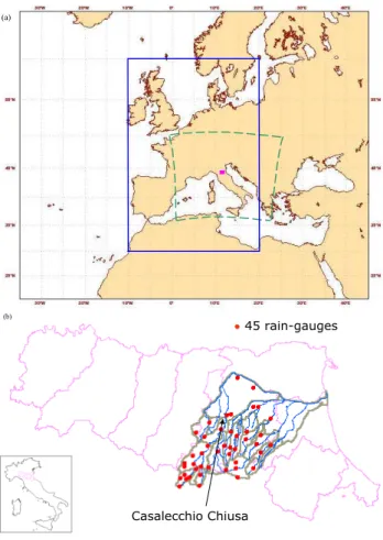
In this work, the implementation of the analogue method is proposed as follows. Based on the research of Cacciamani et al. (1989 and 1991) and Obled et al. (2002), the geopo-tential height (Z) at 500 (Z500) and 850 hPa (Z850), the specific humidity (Q) at 700 hPa, the vertical velocity (W) at 700 hPa and several combinations of these (Z500 com-bined with Z850; Z500 comcom-bined with W ; Z500 comcom-bined with W and Q; W combined with Q) are used to charac-terize the atmospheric circulation over Western Europe and East Atlantic. The search for similar synoptic patterns has been performed on an archive of ECMWF (European Cen-tre for Medium-range Weather Forecasts) analyses of these variables at 12:00 UTC, for the period 1990–2000. The do-main area ranges from 10◦W to 20◦E and from to 30◦N to
60◦N, covered by 3721 model grid points with a grid
spac-ing of 0.5◦(Fig. 1a). According to two similarity criteria, S1
score (Wilks, 1995) and Euclidean Distance (hereafter ED), a certain subset of such analogues is singled out and the cor-responding hourly precipitation measurements, recorded for the following 72 h (starting at 12:00 UTC) by the 45 rain-gauges spread over the Reno river basin (Fig. 1b), are ex-tracted and treated as probabilistic hourly precipitation fore-casts. A quality control process has been applied to the
rain-(a)
•
• 45 rain-gauges
Casalecchio Chiusa (b)
Fig. 1. (a) The domain area for the analogue search (blue line),
the integration domain of LAMBO (dashed green line) and the ge-ographic localisation of the Reno river basin (fuchsia rectangle) in northern Italy. (b) In detail, the Reno river catchment area and its sub-catchments, localised in the Emilia-Romagna Region. Dots de-note the 45 raingauges present in the basin.
fall data in order to arrange an homogenous archive, recon-structing data over not-functioning stations and correcting wrong measurements.
The forecasts obtained via this approach (referred here-after as scheme A) have been compared with those provided by an alternative implementation of the method (hereafter, scheme B), which calculates the precipitation forecast time series for the next 72 h following the procedure proposed by Obled et al. (2002). Scheme B uses the same variables to characterize the atmosphere and similarity criteria as scheme A.
The two approaches can be summarized as follows (Fig. 2). In scheme A, each current day DC and each past
analogue day DP is characterized by ECMWF analyses at
12:00 UTC of day D and day D−1. Since different fields (i.e. the same meteorological variable evaluated at two times or different variables evaluated at two times) are considered, the similarity criterion is applied separately, for each selected
field, to days DC and DC−1, thus evaluating each day in
the past, DP i, as analogous to day DC and the day prior
to DP i (DP i−1) as analogous to day DC−1. Finally, the
sum of the individual similarity criterion values is consid-ered in sorting the sample of analogues available in the his-torical archive. In this way, it may happen that a certain pair of days DP x and DP x−1, with a total analogy degree that
is higher than that of other day pairs, is chosen as member of the N -member subset of analogues from the data archive, even though the individual analogy degrees of day DP x or
day DP x−1 are not among the first N analogues of day DC
and day DC−1, respectively. Afterward, the hourly
precipi-tation forecast is obtained for the next 72 h by considering the raingauge measurements recorded starting from 12:00 UTC of the selected analogue day DP x. Using different
observa-tion times, within the framework of procedure A, the analogy involves the change in time of circulation patterns observed in the last 24 h.
In scheme B, the days Dc and Dp are characterized by
ECMWF analyses at 12:00 UTC of day D and the corre-sponding forecasted fields at +24, +48 and +72 h (i.e. the ECMWF forecasts issued on each day D for the following
D+24, D+48 and D+72 forecast range) since the analogue search is updated every 24 h. In this scheme, different fields (i.e. the same meteorological variable evaluated at two times or different variables evaluated at two times) are also eval-uated within the analogue search process. Thus, the overall criterion used to select the analogue dates for each forecast range is simply the sum of the individual similarity criterion values computed field by field. In detail, for the current day
DC the analogue search is performed for the first forecast
range, i.e. +0–24 h, by comparing, separately, the ECMWF analysis of day DCand the ECMWF model forecast at +24 h
issued on day DC with the corresponding field of each past
analogue day DP i; the hourly precipitation forecast is
ob-tained by considering the raingauge measurements recorded starting from 12:00 UTC of the selected analogue day DP1
for the next 24 h (i.e. the hourly precipitation observed be-tween 12:00 UTC day DP1and 12:00 UTC day DP1+1). For
the next forecast range, i.e. +24–48 h, the analogy is searched for by comparing, separately, the ECMWF forecast issued on day DC for days DC+1 and DC+2 with the
correspond-ing field of each past analogue day DP i; whenever a certain
day DP2 is selected as analogous, the hourly precipitation
forecast is obtained by considering the raingauge measure-ments recorded starting from 12:00 UTC of day DP2+1 for
the next 24 h (i.e. the hourly precipitation observed between 12:00 UTC day DP2+1 and 12:00 UTC day DP2+2). The
analogy for the forecast range +48–72 h is searched for by comparing, separately, the ECMWF forecast issued on day
DCfor days DC+2 and DC+3 with the corresponding field of
each past analogue day DP i; whenever a certain day DP3is
selected as analogous, the hourly precipitation forecast is ob-tained by considering the raingauge measurements recorded starting from 12:00 UTC of day DP3+2 for the next 24 h (i.e.
historical archive ECMWF analyses and
forecasts historical archive hourly raingauge recordings t P DPx-1 DPx DP1 DP1+1 DP2+1 DP2+2 DP3+2 DP3+3 scheme A scheme B t P t P
The precipitation forecast current day Dc Dc-1 Dc Dc+1 Dc+2 Dc+3 ECMWF analyses ECMWF forecasts t The analogue search
historical archive ECMWF analyses and
forecasts historical archive hourly raingauge recordings t P DPx-1 DPx DP1 DP1+1 DP2+1 DP2+2 DP3+2 DP3+3 scheme A scheme B t P t P
The precipitation forecast current day Dc Dc-1 Dc Dc+1 Dc+2 Dc+3 ECMWF analyses ECMWF forecasts t The analogue search
historical archive ECMWF analyses and
forecasts historical archive hourly raingauge recordings t P DPx-1 DPx DP1 DP1+1 DP2+1 DP2+2 DP3+2 DP3+3 scheme A scheme B t P t P
The precipitation forecast current day Dc Dc-1 Dc Dc+1 Dc+2 Dc+3 ECMWF analyses ECMWF forecasts t The analogue search
historical archive ECMWF analyses and
forecasts historical archive hourly raingauge recordings t P t P DPx-1 DPx DP1 DP1+1 DP2+1 DP2+2 DP3+2 DP3+3 scheme A scheme B t P t P
The precipitation forecast
scheme A scheme B t P t P t P t P
The precipitation forecast current day Dc Dc-1 Dc Dc+1 Dc+2 Dc+3 ECMWF analyses ECMWF forecasts t current day Dc Dc-1 Dc Dc+1 Dc+2 Dc+3 ECMWF analyses ECMWF forecasts current day Dc Dc-1 Dc Dc+1 Dc+2 Dc+3 ECMWF analyses ECMWF forecasts current day Dc Dc-1 Dc Dc+1 Dc+2 Dc+3 ECMWF analyses ECMWF forecasts t The analogue search
Fig. 2. Sketch of the analogue-based approach: the analogue search and the precipitation forecast selection. Comparison among schemes A
and B.
the hourly precipitation observed between 12:00 UTC day
DP3+2 and 12:00 UTC day DP3+3). Finally, the hourly
pre-cipitation forecast for the following three days is obtained by joining, for each forecast range, the 24-h series of raingauge measurements recorded during the selected subsets of past analogous days, to achieve the 72-h QPF time series.
The above description points to the fact that, the analogy obtained by procedure B is based on a change in the course of circulation patterns forecasted for the next 24–72 h, and not those observed in the previous 24 h, as in scheme A.
In the present work, the analogue search has been limited to a ten-year period, in order to ensure the availability of a complete and homogenous archive of hydro-meteorological data, appropriate for the study purposes. Again, it is impor-tant to point out, that this restriction could be a limitation to an operational implementation of the analogue approach, if used to support civil protection authorities in their decisions. In fact, the analogue approach is aimed at selecting a certain
nnumber of events (here, n ranging from 15 to 50). How-ever, if a 10-year return rainfall were to occur, there would be little chance of observing it 50 times in 10 years (Obled et al., 2002). The return time of the rainfall event which forecasters are interested in is commonly related to specific warning and alarm thresholds, defined by stakeholders and dependent on meteorological and hydro-geological features of the catch-ment in question. For the Reno river basin, the civil pro-tection authorities have adopted values ranging from 2 to 20 years according to the alert level and the current soil moisture conditions.
2.2 The meteorological model
The rainfall forecasts used in this work were provided by the Limited Area Model BOlogna (LAMBO). This model was the ARPA-SIM (the Regional Hydro-Meteorological Service of the Emilia-Romagna Region) operational atmo-spheric model until 2004. It is a grid-point, split-explicit, primitive equation hydrostatic model, based on an early ver-sion of the NCEP ETA Model (Mesinger et al., 1988). At ARPA-SIM, the operational suite was based on two consecu-tive LAMBO runs: the coarser one was at about 40 km of horizontal resolution and 21 vertical levels on terrain fol-lowing sigma-coordinates. The initial conditions were pro-vided by the ECMWF operational analysis, interpolated to LAMBO resolution; the boundary conditions were provided by the ECMWF operational forecast, available every 6 h throughout all integration time. The integration region cov-ered approximately the area 4◦W–29◦E, 33◦N–52◦N. The
higher resolution run had an horizontal resolution of about 20 km and the integration domain (Fig. 1a) covered the Ital-ian peninsula and the Alpine region, with 32 vertical levels again on terrain following sigma-coordinates. Boundary and initial conditions were provided by the coarser run and were updated every 3 h. LAMBO was run twice a day, nested on ECMWF operational runs of 00:00 UTC and 12:00 UTC, the forecast length being 72 and 84 h, respectively. Outputs were provided every three hours.
2.3 The hydrological model
The hydrological model used to generate simulated dis-charges is the TOPKAPI (TOPographic Kine-matic APprox-imation and Integration) model (Todini and Ciarapica, 2002), a physically-based distributed rainfall-runoff model, applica-ble to different spatial scales, ranging from the hillslope to the catchment, that maintained physically meaningful values for the model parameters at increasing scales. The parame-terisation is relatively simple and parsimonious. It couples the kinematic approach with the topography of the catch-ment and transfers the rainfall-runoff processes into three ‘structurally-similar’ zero-dimensional non-linear reservoir equations. Such equations derive from the integration in space of the non-linear kinematic wave model: the first repre-sents the drainage in the soil, the second reprerepre-sents the over-land flow on saturated or impervious soils and the third rep-resents the channel flow.
The parameter values of the model are shown to be scale independent and obtainable from digital elevation maps (DEM), soil maps and vegetation or land-use maps in terms of slopes, soil permeabilities, topology and surface rough-ness. Land cover, soil properties and channel characteristics are assigned to each grid cell, which represents a computa-tional node for the mass and the momentum balances. The flow paths and slopes are evaluated from the DEM, accord-ing to a neighbourhood relationship based on the principle of minimum energy.
The evapo-transpiration is taken into account as water loss, subtracted from the soil water balance. This loss can be a known quantity, if available, or it can be calculated using temperature data and other topographic, geographic and climatic information. The snow accumulation and melt-ing (snowmelt) component is driven by a radiation estimate based upon the air temperature measurements.
A detailed description of the model can be found in Liu and Todini (2002).
For the implementation of the model over the Reno river basin, the grid resolution is set to 1000 m×1000 m. The cal-ibration and validation runs have been performed using the hourly meteo-hydrological data-set available from 1990 to 2000. The calibration process did not use a curve fitting pro-cess. Rather, an initial estimate for the model parameter set was derived using values taken from the literature. Then, the adjustment of parameters was performed according to a sub-jective analysis of the discharge simulation results. The sim-ulation runs performed for the present work have been car-ried out exploiting different techniques to spatially distribute the precipitation data (forecasts and raingauge observations) onto the hydrological model grid. The Thiessen polygon method was applied to interpolate the irregularly distributed surface observations, whereas the rainfall fields predicted by LAMBO were downscaled to each pixel of the hydrological model structure by assigning to the value of the nearest at-mospheric model grid point.
2.4 The study area
The Reno river basin is the largest in the Emilia-Romagna Region, measuring 4930 km2. It extends about 90 km in the south-north direction, and about 120 km in the east-west di-rection, with a main river total length of 210 km. Slightly more than half of the area is part of the mountain basin. The basin is divided into 43 sub-catchments (Fig. 1b). The moun-tainous part, crossed by the main river, covers 1051 km2up to Casalecchio Chiusa, where the river reaches a length of 84 km starting from its springs. This upper catchment ex-tends about 55 km in the south-north direction, and about 40 km in the east-west direction. It follows a foothill reach about 6 km long, characterised by a particular hydraulic im-portance since it has to connect the regime of mountain basin streams with the river regime of the leveed watercourse in the valley. Contributing to the importance of this reach is the fact, that it extends practically to within the city limits of Bologna. Then, the valley reach conducts the waters (en-closed by high dikes) to its natural outlet in the Adriatic Sea, flowing along the plain for 120 km. In the valley reach, the transverse section of the Reno river is up to about 150–180 m wide.
The altitude of 44% of the area is below 50 m, 51% is char-acterized by an altitude from 50 m up to 900 m, and the re-maining 5% is between 900 and 1825 m.
The concentration time of the watershed is about 10–12 h at the Casalecchio Chiusa river section and about 36 h when the flow propagates through the plain up to the outlet. In this work, the observed and simulated discharges are evaluated at Casalecchio Chiusa, the closure section of the mountainous basin (hereafter “Reno river basin” refers only to this upper zone of the entire watershed). In practice, a flood event at such a river section is defined when the water level, recorded by the gauge station, reaches or exceeds the value of 0.8 m, corresponding to the warning threshold. The pre-alarm level is set to 1.6 m.
3 Analogue-based QPFs
A statistical analysis has been performed in terms of mean error (hereafter ME) and root mean-squared error (here-after RMSE) over the hourly analogue-based QPFs provided for the fall season (restricted to the period 4 September–29 November due to data availability in the meteo-hydrological historical archive at ARPA-SIM) of each year within the pe-riod 1990–2000, searching for the relative analogue subset on the remaining years. These measures are useful for compar-ing two or more solutions that have been adopted to make the same prediction, although they do not indicate whether these are reliable enough to be used (Carter and Keislar, 2000). This statistical analysis is addressed not only to test the two criteria of similarity, but also the influence of the different
1990-2000 Mean Error ED -0.2 -0.1 0 0.1 0.2 0.3 0 12 24 36 48 60 72 forecast range m m Z ZZ ZW ZWQ WQ WQred Wred W
rnd mean obs prec
(a) 1990-2000 Mean Error S1 -0.2 -0.1 0 0.1 0.2 0.3 0 12 24 36 48 60 72 forecast range m m Z ZZ ZW ZWQ WQ WQred Wred W
rnd mean obs prec
(b)
Fig. 3. Hourly mean error of the 72 h analogue-based
precipita-tion forecast obtained with scheme A, using the fifty-element sub-set. The forecasts cover the fall seasons 1990–2000, for different meteorological variables and combination of them, selected by ED
(a) and S1 (b). The hour 0 in the x-axis corresponds to 12:00 UTC.
meteorological variables, or combination of them, used to determine analogues on the corresponding QPFs.
The results for the eleven years analysed with scheme A, considering a fifty-element analogue subset, are shown in Figs. 3 and 4. Each solution for the analogue-based precipi-tation forecast is identified by the initials of the meteorolog-ical variables used to characterize the synoptic pattern and to define the analogues. In detail, the acronym Z, shown in Figs. 3 and 4 (and used in the sequel of the paper), refers to the forecast based on the analogues of geopotential height at 500 hPa; ZZ to the combination of the previous variable with the same field at 850 hPa; W to the vertical velocity at 700 hPa; ZW to the combination of geopotential height at 500 hPa and vertical velocity at 700 hPa; ZWQ to the com-bination of geopotential height at 500 hPa, vertical velocity at 700 hPa and specific humidity at 700 hPa; and WQ to
1990-2000 RMSE ED 0.5 1 1.5 2 0 12 24 36 48 60 72 forecast range m m Z ZZ ZW ZWQ WQ WQred Wred W rnd (a) 1990-2000 RMSE S1 0.5 1 1.5 2 0 12 24 36 48 60 72 forecast range m m Z ZZ ZW ZWQ WQ WQred Wred W rnd (b)
Fig. 4. Hourly root mean-squared error of the 72 h analogue-based precipitation forecast obtained with scheme A, using the fifty-element subset. The forecasts cover the fall seasons 1990–2000, for different meteorological variables and combination of them, se-lected by ED (a) and S1 (b). The hour 0 in the x-axis corresponds to 12:00 UTC.
the combination of vertical velocity and specific humidity, both at 700 hPa. In addition, within the framework of both schemes, a reduced domain area (0◦E–20◦E; 40◦N–50◦N)
has been considered to investigate the analogy only with the variable W and the combination WQ, as these meteorological variables are characterized by a high spatial variability and are more representative of local conditions characterizing an atmospheric circulation pattern: these solutions are labelled with the suffix “red”. The initials “rnd” refer to random se-lected analogues. Figure 3 also displays the mean value of hourly rainfall, averaged over the period 1990–2000, as ref-erence to the error magnitude.
To calculate ME and RMSE, the difference between fore-cast and observed hourly precipitation is calculated for each raingauge and each analogous day. Subsequently, the
er-Table 1. Classification of hourly rainfall for the computation of
RPS.
class rainfall amount (mm/h)
1 0 2 0–0.4 3 0.4–1 4 1–3 5 3–6 6 6–15 7 15–30 8 30–50 9 50–75 10 >75
ror for each forecast hour is averaged for all the raingauges and analogues, considering all days of each fall season. No weighting procedure to consider the analogy degree of each analogous day has been applied in the computations.
The analysis shows that the analogue precipitation esti-mates are unbiased and the RMSE values are quite similar for both analogy criteria if Z500 is considered. However, if Z500 is not considered, the analogue precipitation fore-casts exhibit a bias with a trend when sorted by ED, while no trend and bias are observed when analogues are selected by S1. Furthermore, the smallest values of RMSE are due principally to the best prediction of no-rainy events when the analogy criterion is the ED. This result does not occur if ana-logues are selected by S1. Finally, a daily cycle with peaks corresponding to the most rainy hours is evident.
The statistical analysis performed over the hourly analogue-based QPFs using scheme B provide outcomes that are substantially equivalent to the above-mentioned ones. Only the trend, observed when analogues selected without considering Z500 are sorted by ED, is less noticeable (not shown).
The verification of these probability forecasts over the eleven years has been carried out using the Ranked Proba-bility Score (Epstein, 1969; Murphy, 1971), particularly ex-ploited as evaluation criterion to determine which meteoro-logical field provides a better estimation of precipitation, as well as to assess the relevance of the two similarity criteria and the optimal size of the analogue ensemble. This measure considers a number of categories (J) over which the proba-bilistic forecast is distributed. The RPS for a perfect fore-cast is equal to 0. Forefore-casts that are less than perfect receive scores that are positive numbers, while the worst possible score is J-1. Therefore, the closer the forecast is to 0, the more useful is the forecast. The number of classes and the class boundaries should be suitably defined, counting for the climatology and extension of the area involved, as well as the accumulation period of the precipitation.
Fall 1990-2000 fc 00-24 ED 23 24 25 26 27 28 29 Z ZZ ZW ZWQ WQ WQred Wred W rnd field R P S * 1 0 0
50anl 30anl 15anl
50anl 30anl 15anl
____ scheme A _ _ _ scheme B (a) Fall 1990-2000 fc 00-24 S1 23 24 25 26 27 28 29 Z ZZ ZW ZWQ WQ WQred Wred W rnd field R P S * 1 0 0
50anl 30anl 15anl
50anl 30anl 15anl
____ scheme A _ _ _ scheme B
(b)
Fig. 5. RPS comparison of the optimal analogue subset size,
per-formed with the first 24 h of precipitation forecast provided for schemes A and B by analogues corresponding to different meteo-rological variables, and combination of them, selected by ED (a) and S1 (b).
Considering all the aforementioned aspects, ten classes of hourly rainfall (details of which are shown in Table 1) have been defined, suitable to the regime of precipitation charac-terizing the Reno river basin. The statistical study has been performed considering three forecast ranges (+0–24 h; +24– 48 h; +48–72 h). The result, in terms of RPS for the entire period (1990–2000), is conveyed by the mean value of RPS obtained by averaging the RPS values, calculated for each autumn season, corresponding to the hourly forecasts issued by a certain analogue subset for each raingauge and event.
Different aspects of the scheme optimisation, based on the computation results achieved for the first forecast range pe-riod (displayed in Fig. 5, with the RPS values multiplied by 100) have been evaluated. With respect to the sensitivity of the analogy criterion, the S1 score’s forecasting ability ap-pears to be similar for all the predictor variables. On the other hand, the ED tends to prefer analogues sorted involv-ing Z500. The analogue ensembles selected not considerinvolv-ing
Z500 are characterized by higher RPS values, near to the ran-dom subset. Examination of the optimal size of the analogue ensemble shows slight differences when the number of ana-logues is reduced from 50 to 30 (for both similarity criteria and schemes), whereas the 15-member sample shows higher RPS values. In particular, in case of the S1 (Fig. 5b), the RPS values of the fifty-element subsets are always lower for both schemes; at most, they result similar to those related to the thirty-element subset for few solutions. The same outcome is obtained in case of the ED (Fig. 5a) for solutions related to analogues which consider the variable Z500. In case of the ED, however, the thirty-element subset is clearly preferable in both schemes only for the solutions Wred and WQred; for the solution W, the RPS values of the two different-sized subsets are substantially equivalent for both schemes, while for the solution WQ the thirty-element subset performs better only within the framework of scheme B. In view of these re-sults, and considering that the analogues which involve Z500 show better performance in terms of QPFs, it is preferable to choose the fifty-element subset. This subset also includes more variability.
The fifty-element analogue subset, here shown to be op-timal for obtaining a better QPF, confirms the outcomes of previous studies (Cacciamani et al., 1989 and 1991; Obled et al., 2002). It represents a compromise between the need to encompass the possible occurrence of rare events while avoiding the delivery of the contents of the whole archive, i.e. a climatological forecast. However, it must be stressed that this conclusion is highly dependent on the size of the learning sample, and therefore valid only for the available archive in its present state. The result also depends on the score selected to measure performance: the RPS tends to favour rather spread forecasts to “sharper” forecasts; another score, more favourable to fine distributions, could suggest a smaller number of analogues (Obled et al., 2002).
As to the ensemble spread, it is worth to point out that, given a certain historical archive, the spread of the analogue-based QPFs is mainly influenced by the atmospheric situa-tion over the space domain considered. As example, for the study area selected in the present work, when a geopotential ridge is well located over the Italian peninsula, the probabil-ity to have rainfall events is quite low over the Reno river basin. In this case, the analogue subset will be characterised by a fairly limited spread, independent of or only slightly influenced by the ensemble size and the similarity criterion adopted to sort analogues. On the other hand, when a through is crossing the domain area, the probability that precipitation occurs over the Reno river catchment depends on the geopo-tential phase. In this case, the analogue subset will probably be characterised by a larger spread, more influenced by the ensemble size and the similarity criterion.
Regarding the meteorological variable which provides a better estimation of precipitation, both analogy criteria show that, the best forecast (lower values of RPS) is the one that considers both Z at 500 hPa and W at 700 hPa (and also
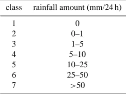
to-Table 2. Classification of daily rainfall for the computation of RPS.
class rainfall amount (mm/24 h)
1 0 2 0–1 3 1–5 4 5–10 5 10–25 6 25–50 7 >50
gether with Q at 700 hPa). The scheme comparison reveals slightly lower values for method B, even though the differ-ences can be regarded as negligible, since the RPS value (be-ing multiplied by 100) can range from 0 to 900 in this analy-sis.
For the next forecast ranges (the +24–48 h and +48–72 h periods), the conclusions are substantially equivalent to the aforementioned ones. In addition, a performance decay is more evident in scheme A than in scheme B. The decrease in forecast accuracy is the greatest between the first and the second lead-time period, while the performances of differ-ent solutions are comparable with those of random selected analogues in the third period.
To optimize the analogue method before its application for hydrological purposes, a further test has been carried out to assess the influence of the domain size on the qual-ity of analogue-based QPFs, extending the area over which the analogy is investigated (20◦W–30◦E; 30◦N–60◦N,
cov-ered by 6161 model grid points). This test has been per-formed only for scheme A. The results (not shown) do not reveal remarkable differences with respect to those related to the domain covered by 3721 model grid points (described at Sect. 2.1). Obviously, the solutions Wred and WQred have not been involved in this additional test.
The statistical study in terms of RPS has been repeated by considering the daily analogue-based QPFs (seven classes of 24-h accumulated rainfall, details of which are shown in Ta-ble 2, have been defined following the same criterion adopted for the hourly precipitation). It confirms the aforemen-tioned outcomes regarding the hourly forecasts about differ-ent facets of the scheme optimisation (results not shown).
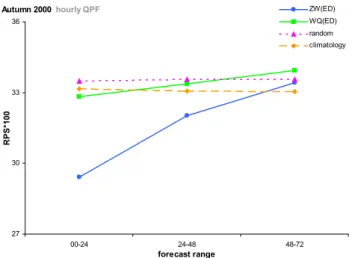
In order to have some reference levels for the analogue-based QPFs, for the 2000 autumn season these have been compared to poor-man forecasting methods (climatology and persistence), with respect to the fifty-member analogue sub-set. In case of the hourly rainfall forecast, the results obtained in terms of RPS (displayed in Fig. 6 for scheme A) show, that the best analogue-based solution (i.e. by consensus of both schemes, the analogues of ZW selected with ED) pro-vides a higher forecast skill as compared to climatology up to the 48th forecast hour. Its performance decays during the
Autumn 2000 hourly QPF 27 30 33 36 00-24 24-48 48-72 forecast range R PS* 1 0 0 ZW(ED) WQ(ED) random climatology
Fig. 6. RPS comparison of the performance of hourly QPFs
pro-vided by the best and worst analogue-based solutions of scheme A (i.e. respectively, the fifty-member analogue subset of ZW and WQ, both selected by ED), fifty random selected analogues and climatol-ogy, as a function of the forecast range (h).
next time range, resembling the climatological forecast. On the other hand, the scores of the worst analogue-based solu-tion (i.e. by consensus of both schemes, the analogues of WQ selected with ED) demonstrate the importance of a suitable selection of the meteorological variable(s) used to investigate the analogy and the usefulness of a scheme-optimisation pro-cess to avoid poor forecast accuracy in the analogue method. The subset of randomly selected analogues shows scores which are rather similar to the climatology. This is quite reasonable, since such past situations are sorted by chance from the available historical data-base, the known climatol-ogy over the target area. With respect to the daily rainfall forecasts (provided by scheme A), for the first 24-h, the low-est forecast skill is given by the persistence as compared to the climatology and the random analogue sample (Fig. 7), confirming the results obtained by Obled et al. (2002). The performances of these latter two methods are similar to one of the worst analogue-based solutions (i.e. analogues of WQ selected with ED).
The deterministic forecast, provided by the meteorolog-ical model LAMBO, has also been compared to the daily analogue-based QPFs obtained with scheme A, for the fifty-member subset. A subjective analysis (not shown) performed on the autumn seasons 1997–2000 indicated, that, generally, the temporal forecasting sequences of daily precipitation pro-vided by LAMBO were better in predicting the non-rainy events than any solution of the analogue-based QPFs (this outcome is more evident for the solutions involving Z500). However, these tended to underestimate the rainfall amount in the case of intense events.
Autumn 2000 daily QPF forecast range +00-24h
40 50 60 70 80 90 100 110
ZW(ED) WQ(ED) random climatology persistence methods providing QPF R PS* 1 0 0
Fig. 7. RPS comparison of the performance of daily QPFs provided
for the first 24 forecast hours by different methods: two analogue-based solutions of scheme A (the fifty-member analogue subset of ZW and WQ, both selected by ED), random selected analogues, persistence and climatology.
4 Discharge forecasts driven by analogue-based rainfall predictions and by LAMBO
The hourly analogue-based QPFs can be used as inputs for the TOPKAPI model, thus generating an ensemble of dis-charge forecasts. A test has been carried out for autumn 2000. A statistical analysis has been performed in terms of RPS on the analogue-driven streamflow predictions issued for the Casalecchio Chiusa river section. The discharge ob-tained by feeding the hydrological model with observed rain-fall was considered as the observation in the computation of the RPS values, thus making the assumption of a perfect hy-drological model forecast. In this way, the attention is fo-cused on the hydrological effects of errors in the QPFs, since the dominant effect influencing the reliability and accuracy of the hydrological prediction is related to the forecast skill of QPFs used as input to the TOPKAPI model.
The statistical study considers three forecast ranges (+0– 24 h; +24–48 h; +48–72 h). The results are expressed as the mean value of RPS, obtained by averaging the RPS values corresponding to the hourly discharge forecasts provided by each analogue-based QPF scenario for every event of autumn 2000. A high number of classes (23), based on the stream-flow regimes characterizing the Reno river basin, has been defined (Table 3), in order to account for a wider range of dis-charge values (corresponding to streamflow regimes mean-ingful for stakeholders and basin management authorities), thus enabling a detailed evaluation of the forecast accuracy (a further test, based on eleven classes only, does not sub-stantially modify the outcomes).
Hydrological simulations, dependent on the outcomes pro-vided by the QPFs verification, have been forced on the fifty-member analogue subset. The results (Fig. 8) confirm, that
Table 3. Classification of discharge values for the computation of RPS. Class discharge (m3/s) 1 <10 2 10–50 3 50–100 4 100–150 5 150–200 6 200–250 7 250–300 8 300–350 9 350–400 10 400–450 11 450–500 12 500–600 13 600–700 14 700–800 15 800–900 16 900–1000 17 1000–1100 18 1100–1200 19 1200–1300 20 1300–1450 21 1450–1600 22 1600–1800 23 >1800
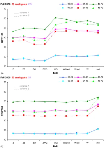
discharge forecasts, driven by QPFs corresponding to ana-logues selected considering Z500, are better than those ob-tained not involving Z500. Particularly, with respect to the sum of RPS values obtained for every forecast range, scheme and analogy criterion, the solution of geopotential at 500 hPa combined with vertical velocity at 700 hPa provide a better estimation of future flows. Similar scores are obtained by the solution which involves the aforementioned two variables and the specific humidity at 700 hPa. These two solutions show the best values of RPS, despite the fact that, the remain-ing solutions involvremain-ing Z500 show differences which can be regarded as negligible since, in this case, the RPS value (multiplied by 100) can range from 0 to 2200 (depending on the number of classes defined). Within the first 24 forecast hours, the performances of discharge simulations based on the two analogue schemes are substantially equivalent. A performance decay with increasing lead-time is evident and more pronounced for scheme A. This result decreases the re-liability of the discharge forecast provided by scheme A for an operational use by civil protection authorities, in case of forecast ranges longer than 24 h. However, this drawback can be partially overcome by exploiting scheme B beyond the first 24 forecast hours.
The impact of the analogy criterion on the selection of the best solution is clear only for ED, whereas the performance of the different solutions are rather similar with S1 (Fig. 8b).
Fall 2000 50 analogues ED 10 20 30 40 50 60 70 Z ZZ ZW ZWQ WQ WQred Wred W rnd field R P S *1 0 0 00-24 24-48 48-72 00-24 24-48 48-72 ____ scheme A _ _ _ scheme B (a) Fall 2000 50 analogues S1 10 20 30 40 50 60 70 Z ZZ ZW ZWQ WQ WQred Wred W rnd field R PS* 1 0 0 00-24 24-48 48-72 00-24 24-48 48-72 ____ scheme A _ _ _ scheme B (b)
Fig. 8. RPS comparison of the performance decay of
analogue-based discharge forecasts provided by schemes A and B, consid-ering the QPFs of the fifty member analogue subset corresponding to different meteorological variables, and combination of them, se-lected by ED (a) and S1 (b).
The ED criterion penalises the discharge forecasts based on analogues independent of Z500, whose RPS values are com-parable to the ones provided by the random analogue sub-set (Fig. 8a). This demonstrates the poor accuracy of such streamflow predictions.
The attained results resemble those corresponding to the QPFs, but the differences among solutions are attenuated. This is because the intermittence of the rainfall signal is dampened by the non-linearity in rainfall-runoff processes. Particularly, the dynamics of the overall soil filling and de-pletion mechanisms and the flood routing play a fundamental role in determining these results.
In addition, the deterministic QPFs, provided by the mete-orological model LAMBO (run at 12:00 UTC) for autumn 2000, have been used as input to the TOPKAPI, evaluat-ing the relevant discharge forecasts in terms of RPS. Even though such a measure is conceived for probabilistic fore-casts, it has been applied to the LAMBO-driven hydrolog-ical runs in order to enable a comparison of the reliability
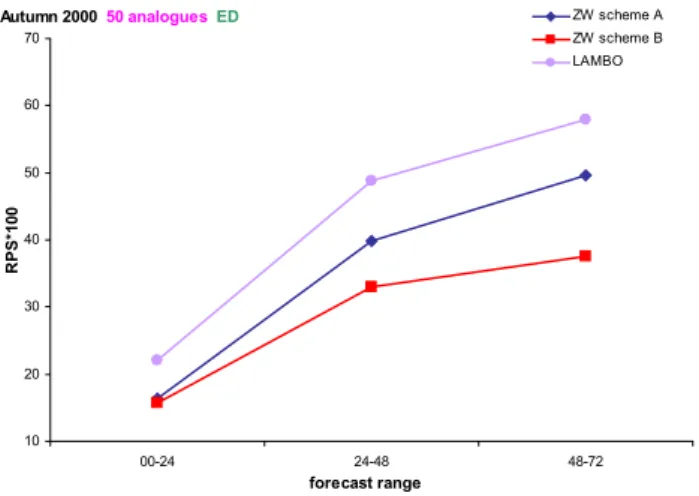
Autumn 2000 50 analogues ED 10 20 30 40 50 60 70 00-24 24-48 48-72 forecast range R P S *1 0 0 ZW scheme A ZW scheme B LAMBO
Fig. 9. RPS comparison of the performance decay of discharge
fore-casts driven by QPFs provided by LAMBO and by schemes A and B considering the fifty-member analogue subset of ZW, selected by ED.
and accuracy of predictions based on the analogue method. The LAMBO scores are worse than the best solution of the analogue method (i.e. the fifty-member analogue subset of ZW, selected by ED), as performed by both schemes A and B (Fig. 9). The poorer forecast skill (higher RPS values) of LAMBO-driven simulations are evident for every cast range, although the deterministic nature of such fore-casts have to be considered in interpreting these results.
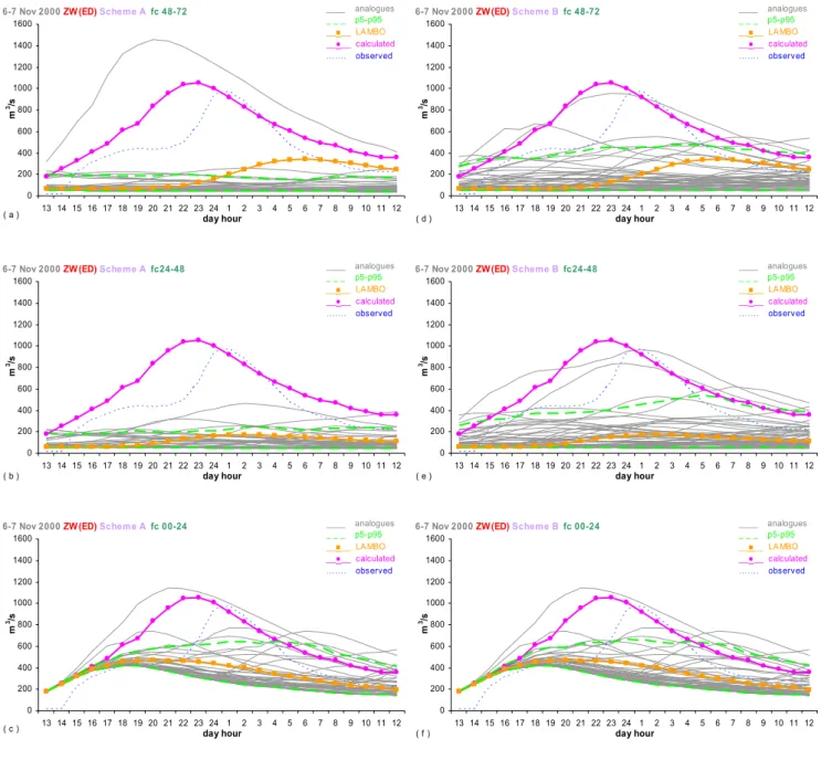
The statistical study performed on autumn 2000 has al-lowed the general evaluation of the performance of the analogue-based discharge forecasts. The following provides a detailed analysis of three case studies, corresponding to the most important flood events occurring during autumn 2000 at the Casalecchio Chiusa river section. In particular, the case studies investigated (all exceeding the warning thresh-old) are: the 6–7 November 2000 event, the 20–21 November 2000 event and the 3–4 November 2000 event. The first one, characterized by a maximum water level of 2.20 m (corre-sponding to a discharge value of about 1200 m3/s), represents the 3rd most critical case in terms of flood event magnitude over a historical archive collecting of events from 1981 to 2004. The second one, characterized by a maximum wa-ter level of 1.55 m (corresponding to a discharge value of about 580 m3/s), represents the 20th most critical case. The last one, characterized by a maximum water level of 1.39 m (corresponding to a discharge value of about 450 m3/s), rep-resents the 31st most critical case. The relevant discharge forecasts, forced with the QPFs provided by analogues of the geopotential field at 500 hPa and the vertical velocity at 700 hPa, selected by ED, are illustrated in Figs. 10–12, for different forecast lead-times, by means of “spaghetti-like” plots and in terms of a percentile confidence interval. The observed discharge, obtained by applying the rating curve available for the Casalecchio Chiusa river section to the
cor-responding water level gauge recordings, is also displayed in order to convey the performance of the TOPKAPI in repro-ducing the Reno river streamflow.
For the 6–7 November 2000 event, the forecast skill of the ensemble provided by scheme A is very limited for the pre-dictions issued 2 and 3 days in advance. The order of mag-nitude of the event is anticipated well enough (even if too enhanced) three days before only by one member (Fig. 10a), but this signal is missed in next forecast range (Fig. 10b). Only the forecast issued 24 h in advance is satisfactory, as several members predict a noteworthy streamflow increase. One member in particular resembles the calculated discharge closely (Fig. 10c). The deterministic run driven by LAMBO underestimates heavily the event at every forecast range. The performance of the hydrological prediction forced with the QPFs provided by scheme B is substantially equivalent to that of scheme A for the first 24 h (Fig. 10f), whereas an improvement of accuracy is evident in the ensembles corre-sponding to the next forecast ranges (Fig. 10d–e).
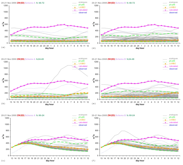
With respect to the second analysed event, the observed discharge is characterized by two peaks, not well repro-duced by the calculated streamflow, which provides a flat-ter signal. The first 24-h forecasts, based on analogues and LAMBO, are only able to detect the first peak flow (Fig. 11c– f), afterwards generally predicting a decrease in streamflow (Fig. 11a–b). For the next lead-times, only the ensembles of scheme B provide a sufficiently informative prediction (Fig. 11d–e).
In the analysis of the 3–4 November 2003 event, the ana-logue ensemble of scheme A reflects the observed and cal-culated discharges during the first forecast range quite well (Fig. 12c), but the variability within the ensemble decreases for the next forecast ranges, missing the flood peak (Fig. 12a– b). Rather, the prediction provided by scheme B shows a still meaningful ensemble spread, with an increasing lead-time (Fig. 12d–e–f). The streamflow prediction based on LAMBO underestimates the event when issued one day in advance, whereas it fails totally for longer lead-times.
For the three case studies analysed, a confidence interval expressed in terms of quantiles corresponding to the non-exceedance probabilities of 5% and 95% is shown, in order to convey the broadest information content of the ensemble possible. Unfortunately, such confidence interval is not able to fully encompass the observed or calculated discharge at every forecast range, the reliability of the interval decay-ing with the increase of lead-time and entity of the event (Figs. 10–12). Within a theoretical framework, the use of confidence intervals should be a more correct approach to assess uncertainty about a discharge forecast and should help stakeholders to interpret results easily. Nevertheless, it may be misleading during extreme events, where the total spread of the forecast may not be conveyed. In case of an extreme event, only few forecast scenarios may able to anticipate the order of magnitude of the peak flow, owing to the limited his-torical archive. A confidence interval based on quantiles will
6-7 Nov 2000ZW (ED) Scheme A fc 48-72 0 200 400 600 800 1000 1200 1400 1600 13 14 15 16 17 18 19 20 21 22 23 24 1 2 3 4 5 6 7 8 9 10 11 12 day hour m 3/s ( a ) ____ analogues _ _ _ p5-p95 __■__ LAMBO __●__ calculated ……. observed
6-7 Nov 2000ZW (ED) Scheme B fc 48-72
0 200 400 600 800 1000 1200 1400 1600 13 14 15 16 17 18 19 20 21 22 23 24 1 2 3 4 5 6 7 8 9 10 11 12 day hour m 3/s ( d ) ____ analogues _ _ _ p5-p95 __■__ LAMBO __●__ calculated ……. observed
6-7 Nov 2000ZW (ED) Scheme A fc24-48
0 200 400 600 800 1000 1200 1400 1600 13 14 15 16 17 18 19 20 21 22 23 24 1 2 3 4 5 6 7 8 9 10 11 12 day hour m 3/s ( b ) ____ analogues _ _ _ p5-p95 __■__ LAMBO __●__ calculated ……. observed
6-7 Nov 2000ZW (ED) Scheme B fc24-48
0 200 400 600 800 1000 1200 1400 1600 13 14 15 16 17 18 19 20 21 22 23 24 1 2 3 4 5 6 7 8 9 10 11 12 day hour m 3/s ( e ) ____ analogues _ _ _ p5-p95 __■__ LAMBO __●__ calculated ……. observed
6-7 Nov 2000ZW (ED) Scheme A fc 00-24
0 200 400 600 800 1000 1200 1400 1600 13 14 15 16 17 18 19 20 21 22 23 24 1 2 3 4 5 6 7 8 9 10 11 12 day hour m 3/s ( c ) ____ analogues _ _ _ p5-p95 __■__ LAMBO __●__ calculated ……. observed
6-7 Nov 2000ZW (ED) Scheme B fc 00-24
0 200 400 600 800 1000 1200 1400 1600 13 14 15 16 17 18 19 20 21 22 23 24 1 2 3 4 5 6 7 8 9 10 11 12 day hour m 3/s ( f ) ____ analogues _ _ _ p5-p95 __■__ LAMBO __●__ calculated ……. observed
Fig. 10. Discharge predictions issued day one (fc 00–24), days two (fc 24–48) and days three (fc 48–72) before the 6–7 November 2000
event, driven by QPFs provided by LAMBO and the fifty-member analogue subset of ZW, selected with ED following the methods A (a, b,
c) and B (d, e, f).
therefore miss useful information. The confidence interval should, however, be more suitable for non-extreme events.
Finally, in a different point of view, the spread of the en-semble, which usually encompasses the hydrological sim-ulation driven by the LAMBO QPF, can be regarded as a measure useful to quantify the uncertainty of the determin-istic forecast, taken as an error-affected “measurement” of the future flow, which does not convey any quantification of the forecast uncertainty. The analogue-based ensemble prediction could be then considered not alternative but
com-plementary to the deterministic one provided by a numerical model, especially when used together to improve real-time flood forecasting. As a matter of fact, several attempts to combine forecasts given by different types of models have been made in hydrology during the last years (Krzysztofow-icz, 1999; Raftery et al., 2005; Todini et al., 2007). Of these, a correction scheme typical of a Kalman filtering approach in scalar form deserves mention (Jazwinski, 1970; Gelb, 1974; Berger, 1980). By applying this approach, each member of the analogue ensemble, considered as our “a priori best
20-21 Nov 2000ZW (ED) Scheme A fc 48-72 0 200 400 600 800 1000 1200 13 14 15 16 17 18 19 20 21 22 23 24 1 2 3 4 5 6 7 8 9 10 11 12 day hour m 3/s ( a ) ____ analogues _ _ _ p5-p95 __■__ LAMBO __●__ calculated ……. observed
20-21 Nov 2000ZW (ED) Scheme B fc 48-72
0 200 400 600 800 1000 1200 13 14 15 16 17 18 19 20 21 22 23 24 1 2 3 4 5 6 7 8 9 10 11 12 day hour m 3/s ( d ) ____ analogues _ _ _ p5-p95 __■__ LAMBO __●__ calculated ……. observed
20-21 Nov 2000ZW (ED) Scheme A fc24-48
0 200 400 600 800 1000 1200 13 14 15 16 17 18 19 20 21 22 23 24 1 2 3 4 5 6 7 8 9 10 11 12 day hour m 3/s ( b ) ____ analogues _ _ _ p5-p95 __■__ LAMBO __●__ calculated ……. observed
20-21 Nov 2000ZW (ED) Scheme B fc24-48
0 200 400 600 800 1000 1200 13 14 15 16 17 18 19 20 21 22 23 24 1 2 3 4 5 6 7 8 9 10 11 12 day hour m 3/s ( e ) ____ analogues _ _ _ p5-p95 __■__ LAMBO __●__ calculated ……. observed
20-21 Nov 2000ZW (ED) Scheme A fc 00-24
0 200 400 600 800 1000 1200 13 14 15 16 17 18 19 20 21 22 23 24 1 2 3 4 5 6 7 8 9 10 11 12 day hour m 3/s ( c ) ____ analogues _ _ _ p5-p95 __■__ LAMBO __●__ calculated ……. observed
20-21 Nov 2000ZW (ED) Scheme B fc 00-24
0 200 400 600 800 1000 1200 13 14 15 16 17 18 19 20 21 22 23 24 1 2 3 4 5 6 7 8 9 10 11 12 day hour m 3/s ( f ) ____ analogues _ _ _ p5-p95 __■__ LAMBO __●__ calculated ……. observed
Fig. 11. As in Fig. 10, but for the 20–21 November 2000 event.
guess”, is optimally combined, in a Bayesian sense, with the discharge forecast based on the LAM model to obtain a new “a posteriori” ensemble of discharge forecasts, characterized by the removal of the bias of the forecast error and by a sig-nificant reduction in the overall uncertainty. Unfortunately, this approach needs a historical archive long enough to prop-erly estimate the errors associated with the different sources of forecast. Thus, this kind of combination could not yet have been applied in the present work, as the available data-set is limited.
5 Conclusions
The present work investigated a methodology provid-ing probabilistic quantitative precipitation forecasts (QPFs) based on analogues. This methodology should be considered as complementary, and not alternative, to the classical deter-ministic approach represented by a NWP model, even when employed jointly to improve real-time flood forecasting. The ability of meteorological models, even the high-resolution ones, to supply reliable and precise rainfall forecast to be used directly for flood forecasting purposes is nowadays still limited. This because large uncertainties, many of which
3-4 Nov 2000ZW (ED) Scheme A fc 48-72 0 200 400 600 800 13 14 15 16 17 18 19 20 21 22 23 24 1 2 3 4 5 6 7 8 9 10 11 12 day hour m 3/s ( a ) ____ analogues _ _ _ p5-p95 __■__ LAMBO __●__ calculated ……. observed
3-4 Nov 2000ZW (ED) Scheme B fc 48-72
0 200 400 600 800 13 14 15 16 17 18 19 20 21 22 23 24 1 2 3 4 5 6 7 8 9 10 11 12 day hour m 3/s ( d ) ____ analogues _ _ _ p5-p95 __■__ LAMBO __●__ calculated ……. observed
3-4 Nov 2000ZW (ED) Scheme A fc24-48
0 200 400 600 800 13 14 15 16 17 18 19 20 21 22 23 24 1 2 3 4 5 6 7 8 9 10 11 12 day hour m 3/s ( b ) ____ analogues _ _ _ p5-p95 __■__ LAMBO __●__ calculated ……. observed
3-4 Nov 2000ZW (ED) Scheme B fc24-48
0 200 400 600 800 13 14 15 16 17 18 19 20 21 22 23 24 1 2 3 4 5 6 7 8 9 10 11 12 day hour m 3/s ( e ) ____ analogues _ _ _ p5-p95 __■__ LAMBO __●__ calculated ……. observed
3-4 Nov 2000ZW (ED) Scheme A fc 00-24
0 200 400 600 800 13 14 15 16 17 18 19 20 21 22 23 24 1 2 3 4 5 6 7 8 9 10 11 12 day hour m 3/s ____ analogues _ _ _ p5-p95 __■__ LAMBO __●__ calculated ……. observed ( c )
3-4 Nov 2000ZW (ED) Scheme B fc 00-24
0 200 400 600 800 13 14 15 16 17 18 19 20 21 22 23 24 1 2 3 4 5 6 7 8 9 10 11 12 day hour m 3/s ( f ) ____ analogues _ _ _ p5-p95 __■__ LAMBO __●__ calculated ……. observed
Fig. 12. As in Fig. 10, but for the 3–4 November 2000 event.
arise because the atmosphere is a chaotic system subject to intrinsic predictability limitations, affect the model outputs.
The study aims to quantify the hydrological forecast un-certainty at each step of the forecast process, accounting for the uncertainty inherent in a precipitation forecast, which when propagated into the hydrological model, can provide a more informative hydrological prediction, useful to be com-municated to, and applied by stakeholders (i.e. end users such as representatives from civil protection authorities).
To fulfil this aim, an analogue-based method to QPF has been applied. The underlying assumption in this forecast-ing method is that similar circulation patterns should provide
similar local effects, e.g. on variables such as precipitation. In this way, the analogy does not have to be investigated on the variable of interest directly, but rather, on meteoro-logical parameters that characterize the synoptic situations, like geopotential height, specific humidity and vertical ve-locity. Practically, the analogue methodology exploits the reliable representation of large scale hydrodynamic variables by meteorological models to derive precipitation forecasts in-directly.
Within this framework, two different implementations of the analogue method have been compared: these schemes differ in the procedure used to calculate the hourly