DOI: 10.1007/s00340-004-1661-9 Lasers and Optics w. kornelis m. bruck f.w. helbing c.p. hauri a. heinrich j. biegertu u. keller
Single-shot dynamics of pulses
from a gas-filled hollow fiber
Swiss Federal Institute of Technology (ETH Zürich), Physics Department, 8093 Zürich, Switzerland
Received: 2 July 2004/Revised version: 2 September 2004 Published online: 20 October 2004 • © Springer-Verlag 2004 ABSTRACTWe present measurements of the performance char-acteristics of few-cycle laser pulses generated by propagation through a gas-filled hollow fiber. The pulses going into the fiber and the compressed pulses after the fiber were simul-taneously fully characterized shot-by-shot by using two kHz SPIDER setups and kHz pulse energy measurements. Output-pulse properties were found to be exceptionally stable and Output-pulse characteristics relevant for non-linear applications like high-harmonic generation are discussed.
PACS42.65.Re; 42.65.Ky; 42.65.Sf; 42.65.Jx
1 Introduction
Widespread use is made today of high-power, ultra-short (5–7 fs) laser pulses generated using the hollow-fiber and chirped mirror compression technique [1, 2]. An important application for such systems is coherent extreme-ultraviolet light generation using high-harmonic generation (HHG) [3, 4]. Crucially, use of a hollow fiber with post-compression has proven so far to be the only method of providing the high intensities and short pulses required to gen-erate isolated attosecond pulses using HHG [5].
While 1 kHz shot-by-shot measurements are technically more demanding than using sample averaging, a shot-by-shot data set allows insights into the causes of the hollow-fiber per-formance. For example, it is a well-known problem that vary-ing only the energy of an ultra-short pulse in the laboratory – while keeping all other properties (e.g. chirp, duration) fixed – is practically impossible. Not surprisingly, exact mechan-isms of the hollow-fiber method therefore have undergone few experimental studies. The present work does not discuss the theory of hollow-fiber compression [6] but presents a study of the parameter dependences of the process.
It is well known that high repetition rate allows rapid data collection and helps combat the possible effects of slow performance drifts inherent in multi-component laser sys-tems and experiments. Fast stochastic fluctuations in output-pulse properties always persist, but are here quantified and exploited to test for interdependences. To date, limited single-shot studies have been carried out for the output of a 10-Hz
u Fax: +41-1-633-1059, E-mail: [email protected]
chirped-pulse amplification (CPA) system [7] and for the pulse-duration fluctuations of the hollow-fiber compressed output of a 1-kHz system [8]. This work presents a study where for the first time both the input pulses to the hollow fiber and the broadband output pulses were characterized simultan-eously and shot-by-shot at 1 kHz. In addition to allowing us to study the shot-by-shot performance of the hollow-fiber tech-nique and of our home-built CPA laser system [9], it was also possible to obtain correlations between the input and output pulses. The electric field of the pulses was measured simultan-eously and shot-by-shot using SPIDER (spectral phase inter-ferometry for direct electric field reconstruction) [8, 10, 11]. Complete characterization of both the input and the output of the hollow fiber makes it possible to study the technique in its own right by separating effects stemming from the ampli-fier fluctuations from the non-linear processes occurring in the fiber.
In Sect. 2 we present our experimental setup and describe the different kHz measurement schemes that were used; in Sect. 3 we present a characterization of the pulses from the amplifier, in Sect. 4 a characterization of the hollow-fiber compressed pulses and finally in Sect. 5 correlation studies between the driving pulses entering the fiber and the com-pressed pulses emerging from the fiber.
2 Experimental setup and methods
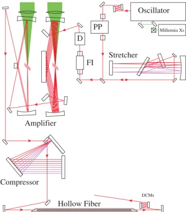
In our experimental setup (Fig. 1) a CPA system produced 30-fs pulses at a repetition rate of 1 kHz with an en-ergy of 870µJ (described below). The amplifier output was focused into a 400µm inner diameter hollow-core fiber filled with 330 mbar of argon. In the hollow fiber a broadening of the optical spectrum occurred and the resulting spectra were compressed by chirped mirrors to about 6.3 fs. We used two single-shot kHz SPIDER systems to measure the spec-tral phase for every single pulse entering the hollow fiber as well as every compressed pulse behind the chirped mirror compressor (Fig. 2). Two fast spectrometers, capable of kHz single-shot operation, measured simultaneously the optical spectra of the pulses entering and exiting the fiber. The pulse energies were also recorded shot-by-shot before and after the hollow fiber. The influence of beam-pointing instabilities was monitored at a kHz rate.
FIGURE 1 CPA laser system: the seed pulse from the oscillator was sent through the pulse picker (PP), which reduced the repetition rate to 1 kHz before being stretched to 200 ps in an all-reflective grating stretcher. After passing through a Faraday isolator (FI) and an acousto-optic programmable dispersive filter (D), the first amplification stage was a cryogenically cooled nine-pass amplifier. The second stage was a two-pass amplifier. A grating compressor reduced the pulse duration to sub-30 fs, which was delivered to the hollow fiber for spectral broadening. Finally, doubly-chirped mirrors (DCMs) recompressed the output
The knowledge of the pulse spectrum, spectral phase (SPI-DER, see below) and energy allows for the complete recon-struction of the electric field of the pulse except for the carrier-envelope (CEO) phase. This permits complete characteriza-tion of every single pulse from the amplifier before entering the hollow fiber and after recompression. In this way we were able to study the fluctuations occurring before and after the fiber as well as to look for correlations between them.
FIGURE 2 Schematic of hollow fiber showing setup and measurements performed. A 2% beam splitter (BS) was used to pick off a fraction of the beam coming from the amplifier (see Fig. 1) to measure the optical spectrum and the spectral phase in the first kHz SPIDER setup. Position-sensitive detectors (PSDs) measured horizontal and vertical beam positions at kHz utilizing the reflection of the entry window. Doubly-chirped mirrors (DCMs) compressed the broadened fiber output and the resulting short pulses were measured simultaneously with another kHz SPIDER setup. Photodiodes (PDs) measured energy in and out of the hollow fiber, which was recorded shot-by-shot at 1 kHz; pickoffs were provided by a fused-silica plate (FS) or leakage through a focusing mirror (RFF is a response-flattening filter and ROC stands for radius of curvature)
2.1 Laser system
The two-stage CPA system (Fig. 1) was seeded by a Ti:sapphire oscillator delivering sub-12 fs laser pulses at a repetition rate of 75 MHz. Pulses were picked from the pulse train at a 1-kHz repetition rate by a Pockels cell and stretched to about 200-ps duration by a grating stretcher. An acousto-optic programmable dispersive filter (DAZZLER) [12] was employed to control the spectral phase of the pulses seed-ing the amplifier chain. The two stages were pumped by a frequency-doubled Nd:YLF laser with the energy of 16 mJ divided equally between the two stages. The first amplifier stage was a nine-pass amplifier using triangular geometry. The Ti:sapphire crystal was cryogenically cooled to 90 K to improve beam uniformity. After nine passes the seed of a few nJwas amplified to about 1 mJ. A second stage which con-sisted of a water-cooled two-pass amplifier further increased the pulse energy to 1.8 mJ. A grating compressor delivered 30-fspulses with an energy of 1.2 mJ.
2.2 Single-shot kHz pulse energy measurement
To measure the energy of laser pulses shot-by-shot at a kHz rate, the femtosecond laser pulse was loosely fo-cused onto a large-area silicon photodiode (Thorlabs Det110). A triggered fast gated boxcar integrator circuit (Stanford Re-search Systems SR250) integrated the signal. The acquisi-tion was set up in such a way that the pulse energy could be recorded continuously and single-shot. The broad optical spectra after the hollow fiber required the use of a response-flattening filter (Melles Griot 13FSD001) in front of the pho-todiode. The energy calibration of the photodiodes was car-ried out by measuring the average pulse energy with a con-ventional calibrated power meter. Additionally, a kHz data set was taken with and without the inclusion of a well-known loss (glass plate). Together with the average pulse energy, the lat-ter measurement provided the energy-scale calibration for the boxcar signal, while preserving high resolution.
2.3 Single-shot kHz beam-pointing measurement
In order to measure the beam-pointing stability of the amplifier and its influence on hollow-fiber dynamics, the
horizontal and vertical beam deviations of the driving pulses were measured with two position-sensitive detectors (PSDs) (SiTek 2L4SP), one for each orthogonal direction. The out-put signals of the PSDs were acquired with a digital storage oscilloscope (LeCroy Wavepro 7100) triggered by the laser system. Acquisition was limited to 15 000 consecutive pulses due to the storage capacity of the oscilloscope.
2.4 Single-shot kHz pulse characterization
A detailed description of our single-shot SPIDER setup and further references may be found in [8]. In sum-mary, in each of our two SPIDER setups the two required spectra (pulse spectrum and SPIDER interferogram) were recorded by separate spectrometers fitted with fast line-scan CCD cameras.
A key requirement was that the acquisition was trigger-able in order to make sure that both spectra were recorded at the same time and thus belonged to the same pulse. The acquisition was continuous and only limited by the data-storage capacity. The on-line pulse-reconstruction rate was limited to 50 Hz by the computing power of our hardware. For the correlated pulse measurements at 1 kHz presented here, we therefore deferred the pulse reconstruction to post-processing and acquired only the necessary raw spectra during the measurement.
2.5 Measurement synchronization and pulse properties
To ensure that the individual measurements could be assigned to the same laser pulse, all measurements must be triggered and no shots missed. A master trigger, derived from the pulse picker of the CPA system, triggered the acquisition of all our diagnostics. Synchronization between the different measurement apparatuses was assured by placing measure-ment markers in the form of suppressed pulses at the start and the end of the measurement runs. The markers, generated by the DAZZLER, made it possible to check if each individual measurement had acquired the same number of shots.
For each laser shot, the recorded energy, spectrum and SPIDER interferogram allowed the reconstruction of the spectral phase, temporal pulse profile and temporal phase of the pulses before and behind the hollow fiber. Subsequently, a set of useful characteristic parameters was calculated for each shot, e.g. pulse duration or spectral bandwidth, allow-ing statistical analysis and visualization by time series and histograms. To visualize the complete set of single-shot spec-tra and pulse shapes we used density plots. On a density plot, darker regions are indicative of a smaller spread.
3 Results: amplifier output stability
First we present the part of the whole data set, con-taining 116 273 laser shots over a time interval of nearly two minutes, which describes fully the amplifier stability.
3.1 Amplifier energy
A critical laser pulse parameter that influences the hollow-fiber dynamics is the input-pulse energy, and its time series is shown in Fig. 3. Figure 4 shows a histogram of the
FIGURE 3 Time series of the pulse energy out of the amplifier. 116 273 successive pulses were measured at 1 kHz
FIGURE 4 Histogram of the amplifier output pulse energy. The crosses are the experimental data in a histogram with 100 bins. The continuous curve is a Gaussian fit to the data. It is centered at 869.4 µJ and has a σ of 6.9 µJ
data in Fig. 3. The excellent agreement with a Gaussian fit (solid line in Fig. 4) indicates that the fluctuations were Gaus-sian. The center was at 869.4 µJ and σ (corresponding to the standard deviation) was 6.9 µJ. The σ of the energy fluctua-tions corresponded to 0.8% of the mean pulse energy, making this a laser system with adequate stability to drive the hollow fiber.
3.2 Amplifier spectral characteristics
The measured spectra were used to extract two rel-evant parameters: the spectral width, which determines the transform-limited pulse duration, and the center of gravity of the spectrum, which is related to the center frequency of the pulse. Since FWHM width does not take into account the shape of the spectrum, we chose to calculate the second-order moment of the spectrum instead. The values and statistical characteristics of these parameters are shown in Table 1. The low standard deviations of these parameters show that the am-plifier spectrum is very stable.
Parameter Mean Std. Dev. shot-to-shot
Energy[µJ] 869.4 6.9 2.5
Spectral width[THz] 14.5 0.2 0.2 Central wavelength[nm] 784.3 0.2 0.2 Pulse duration[fs] 29.0 0.7 0.7
TABLE 1 Measurement of amplifier pulse parameters over 116 273 shots at 1 kHz. The shot-to-shot variation is calculated by averaging the absolute difference between two consecutive shots
FIGURE 5 Density plot of the spectral phase of all the amplifier output laser shots in the data set. The small spread of the curve shows that the phase fluctuations are very low
The spectral phases of all the pulses were reconstructed from the SPIDER measurements in the data set, and are shown in Fig. 5 as a density plot. The sharpness of the curve shows that the shape of the phase remains practically unchanged. The fluctuations are thus very small except in the extreme wings, where the spectral intensity is low and the SPIDER re-construction less reliable due to signal-to-noise restrictions. Note that the spectral phase is constrained to zero at two suitably chosen points (approximately at 375 and 400 THz) by subtracting the arbitrary linear contribution which corres-ponds to a temporal shift of the pulse. The plot therefore illustrates the fluctuations in shape of the spectral phase which in turn affect the temporal characteristics of the pulse. 3.3 Amplifier temporal pulse shape
The temporal pulse envelope for all shots is shown in Fig. 6. The intensity FWHM pulse duration was 29.0 ± 0.7 fs, which corresponds to fluctuations less than 0.5%. This demonstrates that despite the small fluctuations in spectral phase, the temporal pulse profile of the amplifier output was very stable.
3.4 Beam-pointing fluctuations
An important issue concerning the propagation of the mode inside the hollow fiber is the beam-pointing insta-bilities, which change the coupling into the fiber and thus
FIGURE 6 Density plot of the temporal pulse envelope of all the laser shots in the data set. The small spread of the curve shows that the pulse envelope is stable
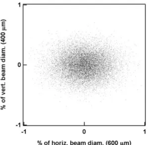
FIGURE 7 Beam position of 15 062 consecutive shots. Both axes are in per cent of the respective horizontal and vertical beam diameters. The beam-pointing fluctuations are well below 1%
exert a considerable influence on the propagation and self-phase modulation. A measurement of the beam pointing of the amplifier output was performed at a kHz rate to investigate possible correlations between the beam position and proper-ties of the short pulses out of the fiber. Figure 7 shows a data sample of 15 062 consecutive shots, where the axes are in per cent of the horizontal and vertical beam diameters. The distri-bution of beam positions was Gaussian in both axes and the peak-to-peak fluctuations were well below 1% of the beam diameter. This system therefore did not need input beam-pointing stabilization.
Table 1 shows the values discussed above and also summa-rizes the spectral characteristics of the amplifier output (not plotted). The low deviations, together with the beam-pointing result, show that the amplifier stability is high. The amplifier fluctuations can be expected to be low enough to be able to study hollow-fiber dynamics in their own right.
4 Hollow-fiber pulse dynamics
We now present measurements of the output of the hollow fiber (diameter 400µm, 330 mbar Ar) taken simul-taneously with the data discussed in Sect. 3. In addition to the parameters examined for the amplifier pulses, we present a number of parameters (temporal chirp and instantaneous frequency at pulse maximum) that are relevant for non-linear processes like HHG and attosecond pulse generation. 4.1 Energy of compressed output
In Fig. 8 the time series for the energy of the hollow fiber compressed pulses is plotted. The initial pulse energy of more than 410µJ drops during 20 s before settling at an aver-age value of 388.7 µJ. This slow saturation-like process was observed every time the laser pulses were switched on and was found to be uncorrelated with the energy, or any other parameter, of the incoming pulses (compare Fig. 3). The first data point corresponds to the first laser pulse to enter the hol-low fiber. We conclude that a shol-low process occurs inside the
FIGURE 8 Time series for the energy after the hollow fiber. The vertical axis is inµJ and the horizontal axis corresponds to measurement time in ms. A salient feature is that the pulse energy drops slowly from a maximum of more than 410µJ to an average of slightly less than 390 µJ within the first 20 s after switching on the laser pulses
FIGURE 9 Histogram of the pulse energy out of the hollow fiber. The dots are the experimental data in a histogram with 100 bins. The continuous curve is a Gaussian fit to the data. It is centered at 388.7 µJ and has a σ of 2.1 µJ
gas-filled hollow fiber and, due to the time scale of the decay, attribute the phenomenon to thermal effects.
Since the first 20 s clearly corresponds to a different regime of operation, in the following we discard the first 22 000laser pulses of the data set in order to study the steady-state behavior of the hollow fiber.
A histogram of the pulse energy from the hollow fiber and after compression is shown in Fig. 9, together with a Gaus-sian fit to the data. The distribution is centered at 388.7 µJ and has aσ of only 2.1 µJ. The energy fluctuations of the pulses from the hollow fiber are 0.5%, which is significantly less than those of the driving laser pulses (0.8%).
4.2 Spectral characteristics of compressed output
The broadening of the spectrum in the hollow fiber is a non-linear process and thus extremely susceptible to fluc-tuations of the input pulses. A density plot of the measured optical spectrum of all the pulses in the steady-state data set is shown in Fig. 10. Some more insight into how important the spectral fluctuations are can be gained from analyzing the spectral width and the central wavelength (center of gravity) of the spectra in Fig. 10; the statistics are shown in Table 2. Both parameters had very little spread, which means that the output spectrum of the fiber was surprisingly stable in view of the non-linear processes at work.
FIGURE 10 Density plot of the output optical spectrum of the hollow fiber. The fluctuations of the spectrum are highest where the curve is broadest. Note that some parts of the spectrum present more variation than others
Parameter Mean Std. Dev. shot-to-shot
Energy[µJ] 388.7 2.1 2.5 Spectral width[THz] 88.8 1.9 0.6 Central wavelength[nm] 775.5 1.6 0.4 Pulse duration[fs] 6.3 0.1 0.1 Chirp[meV/fs] −8.6 2.3 1.3 λmax[nm] 763.0 3.0 1.5
TABLE 2 Measurements of hollow-fiber pulse parameters
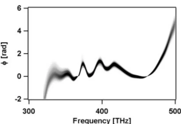
FIGURE 11 Density plot of the spectral phase of the hollow-fiber output. The fluctuations of the phase are most pronounced in the wings where spec-tral intensity is low
The spectral phase is shown as a density plot in Fig. 11 and it is flat and stable for most of the range. Only in the wings is the phase steep and some fluctuations are present. Note that the spectral phase is again constrained to zero at two points by subtracting an arbitrary linear contribution.
4.3 Temporal characteristics of compressed output
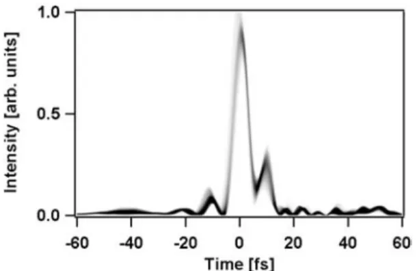
We reconstruct the temporal pulse envelope of the spectrally broadened pulses from the hollow fiber after com-pression by chirped mirrors. The density plot of the pulses (Fig. 12) shows that all the pulses should be suitable for ap-plications such as high-harmonic generation. The mean pulse duration is measured to be 6.3± 0.1 fs (see Table 2). Together with the good energy stability this means that the peak in-tensity, which is an all-important parameter for non-linear applications, is also very uniform.
Clearly, further parameters are needed to describe the properties of the pulses for high-order non-linear optical
phe-FIGURE 12 Density plot of the temporal pulse shape. The pulses are very similar and present little variation in the intensity profile
FIGURE 13 Apparent spread of harmonics 59 and 61 obtained by multipli-cation from a histogram of the instantaneous frequency at the maximum of the pulse, assuming infinitesimal spectral width for each harmonic shot
nomena. It is not only possible to study the pulse envelope but the knowledge of phase and spectrum also gives access to the electric field itself. The measured chirp, i.e. the rate of change of the instantaneous frequency, is shown in Table 2 and we observe that the pulses exhibit a residual negative chirp. The instantaneous frequency at the maximum of the pulse was deduced from the temporal phase of the pulse. It is listed (Table 2) in wavelength unitsλmaxand its average is
763 nm, in order to compare it to the center of gravity of the optical spectrum, which lies at 775.5 nm.
Whileλmaxis similar to the center of gravity of the
spec-trum, it is expected to be more relevant in HHG using few-cycle pulses because higher harmonics are generated near the pulse peak. To illustrate the effect of the fluctuations inλmax
on HHG, we plotted the expected distribution of the positions of harmonics 59 and 61 in Fig. 13 assuming an infinitesimal width of the harmonics. As can be seen, a broad apparent spectral width of the harmonics arises solely from the pulse-to-pulse fluctuations inλmaxof the hollow fiber compressed
pulses. Thus, it could be essential for high-harmonic charac-terization not to average over many shots.
5 Correlation between pulse properties before and after the hollow fiber
The simultaneous measurements provide a much more powerful insight into hollow-fiber dynamics when look-ing for correlations between pulse properties before and after the fiber. From the measured data, we calculated a number
FIGURE 14 Pulse energy behind the hollow fiber versus incoming pulse en-ergy. A linear fit shows a clear correlation: as expected the outgoing energy rises proportionally to the incoming energy
of parameters and performed correlation analyses between pairs. Correlations are visualized most effectively in scatter plots, where strong linear correlations would appear as lin-ear, narrow distributions. Out of the large number of possible correlation plots, we focus on those most relevant for hollow-fiber dynamics.
5.1 Energy correlation
In Fig. 14 the output-pulse energy is plotted against the input energy together with a linear fit. The data showed a clear correlation between the two parameters and, as ex-pected, the higher the incoming energy, the higher the energy coming out of the fiber.
5.2 Spectral characteristics
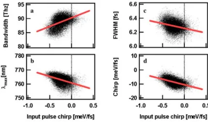
The bandwidth of the broadened spectrum is a cru-cial parameter because it determines the fundamental limit of the compressed pulse duration. We therefore examined the data set to look for input-pulse parameters that strongly cor-relate with output bandwidth. A clear correlation is shown in Fig. 15a, where output bandwidth versus input chirp is plotted. The generated bandwidth was larger for unchirped driving pulses, which is consistent with the chirp being a sen-sitive parameter indicating input-pulse quality. If the chirp vanishes, the pulse is transform limited and has minimal side lobes and thus the spectral broadening in the fiber is improved.
5.3 Temporal characteristics
In the time domain one can observe the same be-havior as in Sect. 5.2. The FWHM pulse duration of the fiber output pulses is also correlated with the chirp of the driving laser pulses (Fig. 15c). The pulses are shorter for lower chirp of the generating pulse, in good agreement with the increased bandwidth under these conditions.
For non-linear applications the wavelength and the chirp at the pulse maximum are relevant parameters, because the dominant interaction takes place at the maximum of the elec-tric field. Both were correlated to the chirp of the driving laser pulse, as shown in Fig. 15b and d. Note that the chirp of the short pulses was negative because their spectral phase was not perfectly flat.
FIGURE 15 The pulse duration, wavelength at the pulse max-imum and the chirp of the hollow fiber compressed pulses versus the chirp of the driving pulse with linear fits
5.4 Other correlations
The broadness of the correlation plots discussed above means that beside the chirp there must have been other factors responsible for the observed variations in the output-pulse characteristics. However, correlations of the out-put spectral and temporal characteristics with the inout-put-pulse energy, duration and spectral width were not found to be sig-nificant. The explanation for these surprisingly absent correla-tions is that the latter parameters are so stable in our amplifier system that the influence of their fluctuations cannot be ob-served as a linear correlation.
We studied the influence of beam pointing on the hollow-fiber output using several shorter complete data sets (due to the limited acquisition capabilities of the beam-position measurement). The results confirmed that in our setup there were no correlations of the compressed pulse properties with input-beam pointing. Again, the absence of any correlation can be attributed to the high beam-pointing stability of the input.
6 Conclusions
We have performed a simultaneous shot-by-shot measurement at 1 kHz of all relevant pulse parameters be-fore and after an argon-filled hollow fiber compression setup. The input pulses provided by a home-made CPA system were found to be very stable. The compressed output pulses after the hollow fiber were 6.3 fs in duration and the fluctuations in the output-pulse properties were found to be correlated with the measured chirp of the input pulses. The hollow fiber improved the energy stability of the input pulses and had ex-cellent spectral stability. The hollow fiber output pulses were analyzed and some parameter fluctuations (other than CEO) affecting sample-averaged HHG spectra were proposed. The conclusion is that single-shot data can provide better insight because they are free of the stochastic shot-to-shot fluctuation, but present demanding challenges to laser characterization and control.
The kHz measurement techniques shown here should in future be complemented by CEO measurements and can then be used to characterize and optimize the performance of sources of isolated attosecond pulses or other sub-6-fs laser sources under development. The dual high-repetition-rate measurement performed here will be of invaluable assis-tance in the optimization and analysis of future experiments, such as dissociation correlation measurements and coherent control experiments. The need to vary pulse parameters with-out relying on stochastic effects can be simply addressed by in future exploiting the powerful pulse control offered by the DAZZLER built into the CPA system presented.
ACKNOWLEDGEMENTS We gratefully acknowledge fruit-ful discussions with P. Schlup and M. Anscombe. We would like to thank M. Roggo from LeCroy for the generous loan of a Wavepro 7100 oscillo-scope. This work was supported by the Swiss National Science Foundation (QP-NCCR) and by ETH Z ¨urich. We acknowledge the support of the EU FP6 programme ‘Structuring the European Research Area’, Marie Curie Research Training Network XTRA (Contract No. FP6-505138).
REFERENCES
1 M. Nisoli, S. De Silvestri, O. Svelto: Appl. Phys. Lett. 68, 2793 (1996) 2 M. Nisoli, S. De Silvestri, O. Svelto, R. Szipocs, K. Ferencz,
C. Spielmann, S. Sartania, F. Krausz: Opt. Lett. 22, 522 (1997) 3 A. McPherson, G. Gibson, H. Jara, U. Johann, T.S. Luk, I. McIntyre,
K. Boyer, C.K. Rhodes: J. Opt. Soc. Am. B 4, 595 (1987)
4 M. Ferray, A. L’Huillier, X.F. Li, L.A. Lompr, G. Mainfray, C. Manus: J. Phys. B: At. Mol. Opt. Phys. 21, L31 (1988)
5 M. Drescher, M. Hentschel, R. Kienberger, G. Tempea, C. Spielmann, G.A. Reider, P.B. Corkum, F. Krausz: Science 291, 1923 (2001) 6 G. Tempea, T. Brabec: Opt. Lett. 23, 762 (1998)
7 C. Dorrer, B. de Beauvoir, C. Le Blanc, S. Ranc, J.P. Rousseau, P. Rousseau, J.P. Chambaret, F. Salin: Opt. Lett. 24, (1999) 1644 8 W. Kornelis, J. Biegert, J.W.G. Tisch, M. Nisoli, G. Sansone, C. Vozzi,
S. De Silvestri, U. Keller: Opt. Lett. 28, 281 (2003)
9 S. Backus, C.G. Durfee III, G. Mourou, H.C. Kapteyn, M.M. Murnane: Opt. Lett. 22, 1256 (1997)
10 C. Iaconis, I.A. Walmsley: IEEE J. Quantum Electron. 35, 501 (1999) 11 L. Gallmann, D.H. Sutter, N. Matuschek, G. Steinmeyer, U. Keller,
C. Iaconis, I.A. Walmsley: Opt. Lett. 24, 1314 (1999)
12 F. Verluise, V. Laude, J.P. Huignard, P. Tournois, A. Migus: J. Opt. Soc. Am. B 17, 138 (2000)