Tectonics controls on fluvial landscapes and drainage development in the westernmost part of Switzerland: Insights from DEM-derived geomorphic indices

Tectonics controls on

fluvial landscapes and drainage development in the

westernmost part of Switzerland: Insights from DEM-derived geomorphic

indices

Omar M.A. Radaideh

, Jon Mosar

Unit of Earth Sciences, Department of Geosciences, University of Fribourg, Switzerland

A R T I C L E I N F O Keywords: Fluvial landscape Geomorphic anomalies Geomorphic indices Hypsometry Inherited faults Reactivation A B S T R A C T

This work focuses particularly on the geomorphological evidence for the tectonic controls on the development of the present-dayfluvial landscapes in the westernmost part of Switzerland. The tectonic deformation was eval-uated on the basis of a combined analysis of several classical geomorphic indices (hypsometric curves and integrals, transverse topographic symmetry index, and channel's bottom gradients) through high-precision DEM processing. A new optimization strategy was applied for defining geomorphic anomalies related to tectonic activity along the channels of three rivers, based on a combined investigation of topographic swath, longitudinal profiles, geological and geophysical observations. The results show that the abnormally high values of hypso-metric integral are spatially occurred on the hanging walls of thrust faults, while abnormally low ones are spatially observed in the same locations of paleo-ice stream pathways. Observations obtained from transverse topographic symmetry index display asymmetries in the most of the studied drainage basins with a predominant SE direction of lateral migration. This direction is in agreement with the dominant dip-direction of the bedding planes within the study area. Abnormal changes in the channel's bottom gradients, which almost coincide in space with pronounced change in the depth of the subsurface geologic layers and in the geophysical properties, are marked by distinct topographic relief in areas where riversflow above blind and emergent faults. Our analysis not only confirms that there is a significant tectonic control on the evolution of drainage systems, but also revealed a possible evidence for the reactivation of some inherited faults.

1. Introduction

The development of Earth's landscapes in tectonically active areas is the result of dynamic interactions between tectonic processes that in-duce vertical and horizontal ground movement, and erosive processes that depend mainly on the lithology and climate among different fac-tors (Armitage et al., 2011;Bishop and Shroder, 2000;Burbank and

Anderson, 2001;Champagnac et al., 2012;Hartley et al., 2011;Norton

et al., 2010a; Trauerstein et al., 2013;Vernon et al., 2009;Whipple,

2004, 2009;Whittaker, 2012). These interactions have a unique

fin-gerprint in the development and evolution of topographic landforms andfluvial systems (Wobus et al., 2006). In other words, the landscapes contain important archival information of the rates and spatial dis-tribution of deformation and erosion (Armitage et al., 2011;Kirby and

Whipple, 2012). Quantitative analysis of such landscapes by using

geomorphic indices can therefore provide valuable information about the genetic link between tectonic and erosion processes, which is an

issue of modern tectonic geomorphology (Mayer, 1986), and help re-cognize late Quaternary tectonic movement (Brookfield, 1998;

Delcaillau, 2001;El Hamdouni et al., 2007;Gao et al., 2016;Harvey

et al., 2015;Hoke et al., 2007;Jackson et al., 1998;Keller and Pinter,

2002;Vojtko et al., 2011).

The Central European Alps region (Fig. 1a), which formed as a result of the collision between the European and African tectonic plates since late Cretaceous times (Schmid et al., 1996), is one of the most im-portant key areas to study the nature of intra-plate compressional de-formations (e.g.,Kley and Voigt, 2008; Ziegler, 1987;Ziegler et al., 1995) and represents an ideal laboratory to describe feedback me-chanisms between tectonic forcing and surface erosion (Champagnac

et al., 2009;Madritsch et al., 2009;Schlunegger and Hinderer, 2002;

Willett et al., 2006). The present-day landscapes of this region and its

northern foreland basin were significantly shaped by several climatic, geological and geomorphical processes, such as glacial erosion, land-slides, and debrisflows (e.g.,Fiore, 2007;Kelly et al., 2004; Korup,

⁎_{Corresponding author at: Unit of Earth Sciences, Department of Geosciences, University of Fribourg, Chemin du Musée 6, CH - 1700 Fribourg, Switzerland.}

E-mail addresses:omar.radaideh@unifr.ch,o.sabbah@ymail.com(O.M.A. Radaideh).

http://doc.rero.ch

Published in "Tectonophysics 768(): 228179, 2019"

which should be cited to refer to this work.

(caption on next page)

2006; Norton et al., 2010a; Salcher et al., 2014; Schlunegger and

Hinderer, 2003; Schlunegger and Norton, 2013; Valla et al., 2011).

While several studies have already highlighted the impacts of climate (Claude et al., 2019;Delunel et al., 2014;Norton et al., 2010a & 2010b;

Schlunegger and Hinderer, 2003; Schlunegger and Norton, 2013),

hillslope (Korup, 2006;Schlunegger, 2002), tectonic uplift (Giamboni

et al., 2004; Korup and Schlunegger, 2008; Madritsch et al., 2009,

2010; Persaud and Pfiffner, 2004), bedrock orientation (Chittenden

et al., 2013;Nunes et al., 2015), and bedrock erodibility (Dürst-Stucki

and Schlunegger, 2013; Korup and Schlunegger, 2008; Kühni and

Pfiffner, 2001; Stutenbecker et al., 2015, 2016) on the evolution of

Alpine landscapes, and/or on denudation rates, no comprehensive analysis of several geomorphic indices has yet been made to clearly explore how the tectonic controls on fluvial landscape development. Thus, the link between tectonics andfluvial landscapes remains rather unclear.

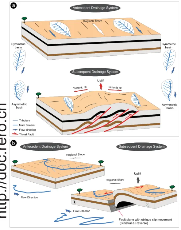
The availability of high-quality digital elevation data, together with the presence of a large variety of tectonic features (i.e., fault zones and fold systems) and the significant spatial variability of topography make the western part of Switzerland (Fig. 1b) a suitable area to conduct morphotectonics analysis. A quite different approach is applied here, based mainly on the combined analysis of several geomorphic indices of the drainage systems. Our hypothesis is that tectonic movements along faults cause substantial topographic andfluvial geomorphic modifica-tions; namely, lateral tilting of the ground surface, topographic re-juvenation, as well as remarkable anomalies in drainage patterns (e.g., abnormal change in the gradients of river channel and a sudden shift in river channel position). We have tested this hypothesis by using (i) hypsometry (area-altitude analysis) that is an effective indicator to quantify uplift and erosion rates of a landscape (Demoulin, 2010;

Hurtrez et al., 1999a, 1999b; Montgomery et al., 2001; Pérez-Peña

et al., 2009; Sternai et al., 2011; Strahler, 1952; Willgoose and

Hancock, 1998); (ii) Transverse Topographic Symmetry Index (TTSI)

that is commonly used to identify areas of a possible tectonic tilting

(Cox, 1994;Cox et al., 2001;Keller and Pinter, 2002;Tsodoulos et al.,

2008); and (iii) longitudinal profiles based on channel's bottom eleva-tion and gradient that are useful to assess short-term tectonic activity (Chen et al., 2003;Delcaillau et al., 2011;Demoulin, 2010;Font et al.,

2010;Hack, 1973). The profiles constructed along the courses of three

rivers (Broye, Glane, and Veyron,Fig. 1b) are also supported by topo-graphic-swath profiles and available geological and geophysical in-formation. The strategy of such combinations is to add important constraints on the origin of any possible geomorphic anomaly and to see whether such anomalies can be attributed to tectonic or any other potentially influencing causes. However, it has been proved that tec-tonics can't always be straightforward, and other factors, particularly deferential erosional strength of the bedrock, glaciation, and hillslope processes, can also induce considerable modifications in the fluvial landscapes (Brocklehurst and Whipple, 2001, 2004;Cox, 1994;Garrote

et al., 2006;Hack, 1973;Korup, 2006;Korup et al., 2010;Lifton and

Chase, 1992; Norton et al., 2010a; Schlunegger, 2002; Seeber and

Gornitz, 1983;Stutenbecker et al., 2016). Based on the above

hypoth-esis, this study aims to quantify the spatial imprints of tectonic de-formation on the development of the present-day topographic land-scapes and the drainage systems of the northern Alpine foreland in the western part of Switzerland.

2. General geological and geographical setting

The Swiss Alps and northern Alpine foreland areas have been the subject of several neotectonic studies. These studies are mainly based on seismicity and stress indicators (e.g.,Cloetingh et al., 2006;Diehl et al., 2018;Marschall et al., 2013;Maurer et al., 1997;Ustaszewski and

Pfiffner, 2008), on geodetic observations (e.g.,Cloetingh et al., 2006;

Kahle et al., 1997; Schlatter et al., 2004;Schlunegger and Hinderer,

2002;Wittmann et al., 2007) and on different geological archives that

include active faults, lake deposits, slopes, and caves (Becker et al.,

2002, 2005;Lemeille et al., 1999;Monecke et al., 2006). The area of

investigation is part of the northern foreland of the Swiss Alps and is situated on either side of the water divide between Rhine and Rhone river systems. It covers an area of 5136.6 km2and lies completely in the westernmost corner of Switzerland between latitudes 46′08′49″ N and 47°14′19″ N and longitudes 5°57′35″ E and 7°17′05″ E. It characterized by abrupt changes in topography with elevation ranges from ~400 m to ~2500 m. It consists of the exposed record of Triassic to Quaternary rocks (Fig. 2), and is mainly characterized by the presence of wide-spread strike-slip faults and fold - thrust belt structures. From a tectonic viewpoint, the study area mainly consists of three large-scale zones, namely: the Jura fold-and-thrust belt, the Molasse Basin, and the Pre-alpes Klippen belt.

The Jura fold-and-thrust belt represents a classic thin-skinned, fold and thrust belt, where a thin Mesozoic sedimentary cover deformed (folded and thrusted) above décollement by“distant push” (Affolter and

Gratier, 2004;Burkhard, 1990;Buxtorf, 1907;Laubscher, 1986, 1992;

Madritsch et al., 2008; Mosar, 1999;Sommaruga, 1997, 1999). The

Jura fold-and-thrust belt, which has a crescent-like shape, is generally divided into three main sectors, which are from north to south: Avant-Monts, the External Jura, and the Internal Jura (Sommaruga, 1997, 1999). The tectonic evolution of the Swiss Molasse Basin is tectonically linked to the formation of the Jura fold-and-thrust belt (Burkhard and

Sommaruga, 1998;Gorin et al., 1993;Mosar, 1999;Pfiffner et al., 1997;

Signer and Gorin, 1995; Sommaruga, 1997, 2011). It is tectonically

subdivided into the Plateau Molasse, and the imbricated Subalpine Molasse. The Plateau Molasse presents areas of relatively little de-formation between the Jura fold-and-thrust belt and the Subalpine Molasse. It is dominated by low-amplitude northeast-trending folds, and several reverse and strike-slip faults with N–S, NW–SE and WNW–ESE trends (Sommaruga, 1997). The strata are characterized by nearlyflat or gentle dips in the areas of Plateau Molasse, but are pro-gressively more tilted toward the Subalpine Molasse. The latter re-presents a narrow deformation zone composed of thrust sheets of Cenozoic rocks that were overthrust by the Penninic Prealpine Klippen and Helvetic nappes (Pfiffner et al., 1997;Pfiffner, 2014). The Swiss Molasse basin consists essentially of four lithostratigraphic units: the Lower Marine Molasse and the Lower Freshwater Molasse, which to-gether form thefirst sedimentary sequence of Oligocene to early Mio-cene age, and the Upper Marine Molasse and the Upper Freshwater Molasse, which together form the second sedimentary sequence of Miocene age (Pfiffner et al., 1997;Schlunegger et al., 1997a, 1997b). The south-eastern corner of the study area is marked by the Prealpes Klippen nappe (Fig. 2a), which consists of several lithologies

(Matzenauer, 2012).

Fig. 1. Geodynamic settings of central and western parts of Mediterranean Basin and surrounding region. (a) Central and western parts of Mediterranean Basin showing the major plate boundaries (Africa and Eurasia), major tectonic systems, and orogenic belts. Insert box in the lower-right corner of the map showing the location of the Mediterranean Basin and surrounding areas. (b) The westernmost area of Switzerland and surrounding regions showing the location of the studied rivers (Broye, Glane, and Veyron). (c) Topographic cross-section showing major topographic features, as well as the change of elevation along a white line A-B in (a). Digital elevation model (30 and 90 m DEMs), global hill shading image (Becker et al., 2009), and bathymetry datasets are provided by the European Environment Agency, e- Atlas, and EMODnet Bathymetry.

3. Materials and methods 3.1. Data collection

Two sources of data were mainly used in this study: elevation and potentialfield (gravity and aeromagnetic) data. The elevation data are composed of high and medium resolution digital elevation models (DEMs). The high-precision DEM with a grid size 2 m (swissALTI3D) provided by the Swiss Federal Office of Topography (Swisstopo). The medium-precision ASTER Global DEM (GDEM) with a grid size ~30 m is a product of METI (Japanese Minister of Economy, Trade and Industry) and NASA (United States National Aeronautics and Space Administration). Ground Bouguer and aeromagnetic maps are pub-lished at a scale of 1:500,000 by Swisstopo. The Bouguer data are part of an extensive gravimetric survey covered the whole Switzerland

during the period 1975–1979. The survey was performed jointly by the Institute of Geophysics of the University of Lausanne (IGPL) and by the Swiss Federal Institute of Technology in Zurich. Almost 80% of the Molasse Basin was covered with a station density ranging between 1 and 3 stations per 1 km square (Klingelé, 1992). The theoretical gravity value was calculated using the International Gravity Formula of 1967. Topographic corrections were computed using a constant density of 2670 kg/m3to a depth of 167 km (Klingelé and Olivier, 1980). The aeromagnetic data are part of a wide aeromagnetic survey covering the Swiss territory between 1978 and 1981 by the Swiss Geophysical Commission. The data were performed at two different flight levels (5000 m and 1680 m above sea level) and along north–south oriented flight lines with a line spacing of 5000 m. The higher flight level cov-ered the whole Swiss territory, whereas the lower one covcov-ered the Molasse Basin and the Jura Mountains. The effect of diurnal variations, Fig. 2. (a) Simplified geological and structural map of the study area in the westernmost part of Switzerland. Geological data provided by the Swiss Federal Office of Topography (Swisstopo). Structural elements map was compiled byGruber (2017). (b) General geological cross-section across Jura Fold-and-Thrust-Belt (JFTB), Plateau Molasse (PM), Subalpine Molasse (SM), and Préalpes (PA). The location of the cross-section is marked by a dashed black line D-D′ in (a). Cross-section based onBurkhard and Sommaruga (1998),Gruber (2017),Madritsch et al. (2008),Mosar (1999), andRigassi and Jaccard (1995). (c) Location map of the study area.

the effect of secular variations, instrument drift, and regional field were removed from the measured data before constructing the total intensity magnetic anomaly map (Klingelé, 1992;Klingelé and Verdun, 2003). 3.2. Methods

Geomorphic responses to tectonic forcing have been examined by combining analyses of drainage basins, and both, swath and long-itudinal river profiles in areas of spatially variable topography. There are two key aspects for our examination:firstly, to compare drainage basins experiencing different levels of uplift/erosion rates and different lateral migration for their main stream trunks, and secondly, to identify any abrupt variations in the stream channel geometry and gradient along their courses. We employed three morphometric parameters to highlight the tectonic effects: (1) hypsometric integral to assess whether the variation in the landscape's topography is the result of the tectonic uplift, and/or other processes such as glacial erosion and contrasts in bedrock erodibility (Lifton and Chase, 1992;Pérez-Peña et al., 2009;

Sternai et al., 2011; Stutenbecker et al., 2016; van Der Beek and

Bourbon, 2007), (2) Transverse Topographic Symmetry index (TTSI) to

quantify the possibility that lateral migration of main stream channels is induced by a tectonic tilting of the land surface (Cox, 1994;Cox et al.,

2001;Garrote et al., 2006;Tsodoulos et al., 2008), and (3) channel's

bottom elevation and gradient (SL index) to detect areas of abrupt changes in river gradients that could possibly indicate the presence of tectonic control (Delcaillau et al., 2011;Peters and van Balen, 2007;

Seeber and Gornitz, 1983). The analysis was combined with geological

field work and available geological and geophysical (gravity and aeromagnetic) data.

3.2.1. Extraction of drainage systems

The automatic derivation of drainage systems (both stream net-works and basins) has recently attracted a considerable attention (e.g.,

Fairfield and Leymarie, 1991; McMaster, 2002; Palacios-Vélez and

Cuevas-Renaud, 1986;Tarboton, 1997;Turcotte et al., 2000). Different

algorithms have been developed to extract drainage systems from a DEM by using GIS tools. D8 is the most popular used algorithm for automatic drainage extraction (e.g., Anders et al., 2009;

Ariza-Villaverde et al., 2013, 2015; Liu and Zhang, 2011; Nigel and

Rughooputh, 2010;Persendt and Gomez, 2015;Turcotte et al., 2000).

This algorithm is specifically relied on determining direction of water flow from every cell in the DEM raster to one of its eight neighbors, either adjacent or diagonal, in the direction of the steepest descending slope (O'Callaghan and Mark, 1984;Tarboton, 1997). It has been im-plemented in ArcHydro Tools v 2.0, toolset for the water resource ap-plications developed to operate within ArcGIS by the University of Texas (Maidment, 2002). These tools were used to extract drainage systems of the study area from a 2 m-resolution DEM based on suc-cessive processing steps that are described elsewhere (ESRI, 2011). 3.2.2. Drainage catchment analysis

A total seventy-four drainage-catchments of mostly higher Strahler orders (Table A.1) were selected to quantify the causal influences of both tectonic uplift and tilt activities on the drainage basin morphology. The catchments were selected in areas characterized by significant measurements of bedding dip azimuths so that the possible tectonic tilt could be well defined.

3.2.2.1. Spatial distribution of hypsometric integrals. Recent studies have shown that hypsometric curves are very useful tools in geomorphic analysis, since they provide important indicators in regions experiencing intensive erosion processes (Chen et al., 2003; Hurtrez

et al., 1999a, 1999b; Luo, 2000, 2002; Montgomery et al., 2001;

Ohmori, 1993;Sternai et al., 2011;Willgoose and Hancock, 1998). The

hypsometric curve describes the relative elevation distribution of a drainage basin and is thus a measure for the shape of a basin (Strahler,

1952).

Determining the hypsometric curve for a 3rd order basin is shown in Fig. S.1a (in the supplementary data), where (H) and (A) represent respectively the maximum height, and the total area of the basin and (x) represents the surface area within the basin above a given line of ele-vation (h).Strahler (1952)linked the shape of the hypsometric curve with three stages of landscape development, namely: youth, maturity and old age (Supplementary Fig. S.1b). These stages characterize weakly eroded regions with convex-up curves, moderately eroded re-gions with S-shaped curves, and significantly eroded regions with concave-up curves.

Pérez-Peña et al. (2008a)present an ArcGIS extension (CalHypso) to

automatically extract hypsometric curves and calculate simple statistic attributes related to these curves (integral, skewness and kurtosis). The hypsometric integral is the area lying under the curve, ranging from 0 to 1. The hypsometric integral value is very close to zero in the areas experienced the highest levels of erosion, whereas it is very close to 1 in weakly eroded areas (Keller and Pinter, 2002;Pike and Wilson, 1971;

Strahler, 1952). The geomorphological significance of the hypsometric

skewness and hypsometric kurtosis are shown byHarlin (1978), where a larger positive value of skewness reflects a greater amount of head-ward erosion in the upper reach of a basin; and a larger value of kur-tosis reveals a more erosion in both upper and lower reaches of a basin. While hypsometry can assess erosion and describes the distribution of elevations within an area, it is possibly unclear whether there is a causal relationship between hypsometry and geological structures. This has led us to suggest the hypothesis that thrust-related fold growth creates a local relief, which is then eroded by rivers incision. We tested this hypothesis by detecting abnormally high values of hypsometric integral and relating them to existing structures, with taking into account the possible impact of other factors.

The hypsometry curves can be used in drainage watersheds of dif-ferent sizes (e.g.,Giaconia et al., 2012;Girish et al., 2016;Luo, 2000,

2002;Mahmood and Gloaguen, 2011;Omvir and Sarangi, 2008).

In-deed the change in dimension of drainage catchments may play a more important influence on hypsometry than the uplift and erosion rates. Because small catchments are generally showing convex-up hypso-metric curves associated with higher hypsohypso-metric integral values ap-proaching 1.0, whereas larger catchments are having concave-up hyp-sometric curves with much smaller values approaching zero (Chen

et al., 2003;Hurtrez et al., 1999a;Willgoose and Hancock, 1998). To

avoid such pitfalls related to changes in catchments scale we calculated hypsometric curves not only for the drainage catchments but also for regular squares of different sizes through using CalHypso (Pérez-Peña

et al., 2008a). Particular attention must also be paid here not only to

the analysis size but also to the resolutions of the DEM used to calculate the hypsometric curves with their attributes. In this context, three dif-ferent regularly spaced grids (1 km, 2 km, and 3 km) with two different resolution DEMs (2 m and 30 m) were analysed. ArcGIS extension Hawth's Analysis Tools (Beyer, 2004) wasfirst employed to create three vector gridfiles with 1 × 1, 2 × 2 and 3 × 3 square kilometres cells. The hypsometric curve and related attributes were then computed for each vector gridfile over both DEMs separately. The hypsometric in-tegral values obtained from each case were then interpolated in order to obtain a continuous surface. In this way, we obtained regularly-spaced grids of the hypsometric integral values for the whole area and quantify the degree of similarity between the results that obtained by using different scale sizes and DEM resolutions.

3.2.2.2. Drainage basin asymmetry. Tectonic tilting of the surface can cause a deflection of the stream channel away from the midline of drainage basin toward one of its sides (e.g.,Keller and Pinter, 2002;

Mathew et al., 2016). The Transverse Topographic Symmetry Index

(TTSI) and Asymmetry Factor are commonly used to differentiate between symmetric and asymmetric drainage basins and to identify whether they had experienced by a possible tectonic tilting (Cox, 1994;

(caption on next page)

Cox et al., 2001;Garrote et al., 2006;Keller and Pinter, 2002;Mahmood

and Gloaguen, 2011;Sboras et al., 2010;Tsodoulos et al., 2008). The

TTSI is described as a ratio (Da/Dd), where Da is the perpendicular distance between the trunk stream to the basin midline, and Dd is the perpendicular distance between the basin midline to the basin margin along the same line. The Asymmetry Factor is defined as the product of ratio (Ar/T) multiplied by 100 (Keller and Pinter, 2002), where Ar is the basin area on the right-side of the trunk stream while facing downstream, and T is the total area of the drainage basin. The Asymmetry Factor and TTSI values are respectively close/equal to 50 and 0 if the river incises along the basin midline, and≠50 and ≈1 if the riverflows near to the basin boundary (Cox, 1994;Cox et al., 2001;

Keller and Pinter, 2002). The absence of tectonic controls can often lead

to develop symmetric basin with Asymmetry Factor≈ 50 and TTSI ≈ 0, whereas the presence of such controls would develop asymmetric basin with Asymmetry Factor≠ 50 and 0 < TTSI ≤ 1 (Cox, 1994; El

Hamdouni et al., 2007;Mahmood and Gloaguen, 2011). Asymmetric

basin often occurs as a result of the tilt of the ground surface caused by uplifting folds and tilting fault blocks (Cox, 1994). Consequently, tilting of the ground surface generally causes the rivers to be laterally migrated toward the steepest gradient in a direction roughly parallel to its original course. Tectonic activity is not unique and other geological and geomorphological factors, such as paleo-slope surface, wedge-shaped channel (Levee) deposits, and coarse-grained alluvial deposits can also develop lateral channel migrations (Cox, 1994;

Garrote et al., 2006).

In many orogenic belts like the Zagros and Himalaya, where there is a significant interaction between the growth of thrust-related folds and drainage system development, the rivers do not onlyflow in a direction roughly parallel to the strike of the fold axes, but also perpendicular to them (e.g., Burberry et al., 2010; Delcaillau et al., 2006; Ghassemi,

2005; Lu et al., 2017;Ramsey et al., 2008;Tucker and Slingerland,

1996;Walker et al., 2011). The rivers thatflow parallel to the axis of

the fold respond to changes in topographic gradient associated with anticlinal growth, by either incise a gorge through the nose of the folds, or by deflected out of their present courses around the tips of the growing folds in the direction of fold propagation (Burbank and

Anderson, 2001;Ramsey et al., 2008). As the result, the rivers

even-tuallyflow perpendicular to the fold crests with a significant change in their direction along the length of the fold (Ramsey et al., 2008). Such rivers combine information about the lateral migration in the upper part of their courses, which is inherited from the initial stages of fold growth, with information about the perpendicular deflection, which is inherited when the rivers bend away from their initial courses in the direction of folds growth. Therefore, determining whether ground surfaces have experienced tectonic tilting is not always straightforward. Despite possible uncertainties, an attempt was made to confirm the hypothesis that tectonic deformation associated with the growth of thrust-related folds cause lateral tilting of the ground surface in a di-rection parallel to the didi-rection of maximum compressive stress. Thus,

evidence on a possible lateral tilting of the ground surface is the pre-sence of channel migration that can be highlighted by TTSI. The TTSI was determined in successive steps using GIS tools and following the method described elsewhere (Cox, 1994;Cox et al., 2001). Due to the undulating and very irregular shapes of the drainage channel, the main stream trunk was divided into discrete segments of the same length (25 m in this case). The ArcGIS's Polygon to Centerline tool (Dilts, 2015) was used to extract a centerline for a given catchment vector layer. A series of transect-lines that were created orthogonally to the stream's segment-lines were divided into two groups; those bound by the stream and centerline (Da), and those bound by centerline and catchment boundary (Dd). The length of the groups Da and Dd, as well as their azimuth values were then calculated. Having the magnitude (the ratio of the length of Da to the length of Dd) and the azimuth values, we were able to graphically represent these data on the polar diagram. To determine the preferred direction of stream migration, the Fisher mean vector with its associated confidence cones were calculated using Stereonet v9.9.6 (Allmendinger et al., 2011; Cardozo and

Allmendinger, 2013). To obtain further information about the spatial

distribution of TTSI magnitudes, a color-coded grid bounding between catchment's midline and main-stream was created for each catchment. An example of calculating the TTSI for the 3rd order catchment (no. 45) that formed part of the Prealps area in the SE corner of the study area is shown inFig. 3b and c. The calculated TTSI vectors (Fig. 3b and c) are significantly concentrated in the NW quadrant of the polar plot and have a mean vector (trend/magnitude) of 305.4°/ 0.20 with a small cone of confidence at the 95% level. The reliability of Asymmetry Factor is questionable, especially when there is an apparent deflection of the main river channel. This can be explained by the catchment no.

14 (Fig. 3d) where its main channel is sharply deflected in the northeast

and southwest directions. The calculated Asymmetry Factor is almost close to the threshold 50 (50.3%), indicating that there is no any sig-nificant migration direction for the principal channel, whereas the calculated TTSI indicates two main directions of migration with mean vector values (trend/magnitude) of N39°E/0.4, and N233°E/0.49. For this reason, the TTSI was only used in this study to infer any possible tectonic tilting.

3.2.3. River longitudinal and topographic swath profiles

To better define the location/source of the geomorphic anomalies, we suggest a new stepwise approach by integrating analysis of several longitudinal profiles along the course of three rivers (Broye, Glane, and Le-VeyronFig. 1b). These riversflow perpendicular to major sub/sur-face structural features over areas characterized by the presence of ubiquitous geological and geophysical (Bouguer gravity and aero-magnetic) data. The profiles have been evaluated based on two dif-ferent aspects: channelfloor gradient and geophysical properties. This integration is also supported by topographic-swath profiles and new geologic model based on stratigraphic and structural interpretation of seismic lines (Gruber, 2017;Meier, 2010). Our objective behind such a Fig. 3. An example showing the calculation of Transverse Topographic Symmetry Index (TTSI). (a) High-resolutionflow direction grid showing surface-water flow paths of 3rd order catchment no. 45. (b) Calculated TTSI via the method explained byCox (1994). Two thick black transect-lines (1&2) enable measurements of the distance between catchment midline to the trunk stream (Da) and from the catchment midline to the respective drainage margin (Dd). Here there are two vectors, each one composed of the magnitude (Da/Dd) and the line azimuth. Polar plot (equal-area, lower hemisphere) visualizing the magnitudes and azimuths of TTSI vectors obtained from transect-lines. The polar plot has TTSI magnitude ranging from 0 in centre, meaning that the streamflowing near the catchment midline, to 1 on the outer margin, implying that the streamflowing near vicinity of catchment margin. Yellow star on the polar plot (a mean Fisher vector) represents the most prominent direction of stream migration. Rose diagram plotted in terms of frequency against TTSI azimuth values expressing preferential directions of channel migration. (c) Color-coded grid showing the spatial distribution of the TTSI magnitude values. Zone with a dark-green color (TTSI close to 0) indicating no lateral migration of the stream away from the catchment's midline whereas those with dark red (TTSI close to 1) highlighting a significant lateral migration of the stream toward the catchment's margin. (d) A critical issue about the accuracy of asymmetry factor (AF) that is not applied in this study. The calculated AF for the catchment no. 14 is very close to 50% (50.29%), indicating there is no dominant direction of migration. Whereas the calculated TTSI shows two prominent directions of migration, NE and SW. (e) Schematic showing geomorphic response of drainage system to tectonic deformation caused by listric faults. When the earth's surface layers were tilted, the main stream was migrated away from the midline of basin toward the down-tilt direction. It is important to note here that other influencing factors, such as variation in rock-type erodibility can also generate similar geomorphic responses. (For interpretation of the references to color in thisfigure legend, the reader is referred to the web version of this article.)

combination is to add important constraints on the origin of any pos-sible geomorphic anomaly.

3.2.3.1. Channel floor-gradient. The spatial changes in the channel's bottom elevation and slope from its headwaters to its estuary are currently the most common indicators used to detect signs of Quaternary tectonic activity. Any rapid change in these properties causes pronounced geomorphic anomaly or knickpoint that represents non-steady state signatures in the river channel geometry. Such anomaly results from several factors, such as lithologic resistance to fluvial erosion, variations in tectonic uplift, changes in stream discharge, changes in local base-level, and rock-slope failures (Bishop

et al., 2005; Brocard and van Der Beek, 2006; Clark et al., 2004;

Delcaillau et al., 1998;Duvall et al., 2004;Gardner, 1983;Hack, 1973;

Hayakawa and Oguchi, 2006;Korup, 2006;Larue, 2007;Norton et al.,

2010a; Ouchi, 1985; Rabin et al., 2015; Radaideh et al., 2016;

Schlunegger, 2002; Seeber and Gornitz, 1983; Stutenbecker et al.,

2015, 2016;Whipple and Tucker, 1999). Thus, the shapes of the river

longitudinal profiles reflect the causal relationship between lithology, fluvial erosion, tectonics, and base level change (Clark et al., 2004;

Delcaillau et al., 1998; Hack, 1973; Kale et al., 2013; Merritts and

Vincent, 1989;Wobus et al., 2006). The concave-up longitudinal profile

indicates that erosion has kept pace with tectonic uplift and thus, the rates of uplift equal the rates of erosion. If the rate offluvial incision is greater than the rates of rock uplift and base-level fall, then the shapes of the profile tend to show a smooth downstream concavity due to increase of sedimentflux. Conversely, if the rate of uplift is greater than fluvial incision, then the shapes of the profile will be convex (Seeber

and Gornitz, 1983).

Several geomorphic indices have been proposed to detect the knickpoint locations along the river courses. Among them, the most commonly used indices are river channel steepness and river channel length-gradient. The channel steepness index is a measure of stream-channel slope normalized to drainage area (Wobus et al., 2006), and follows the equation: S = ksn*A-θref, where S is the channel slope, ksnis

a normalized steepness index, A is the upstream drainage area,θrefis a

reference concavity index. It has widely used to infer relative differ-ences in rock uplift in a variety of landscapes (Chittenden et al., 2013;

Cyr et al., 2010; Fraefel, 2008; Gasparini and Whipple, 2014; Kirby

et al., 2003; Kirby and Whipple, 2012;Norton et al., 2010a; Ouimet

et al., 2009;Safran et al., 2005;Schlunegger et al., 2011;Snyder et al.,

2000;Whipple and Gasparini, 2014).

The channel length-gradient index (also known as SL index) is the product of the channel slope and channel length (Hack, 1973), and is represented as: SL = (ΔH/ΔL)*L, where ΔH is the difference in eleva-tion between the ends of the segment,ΔL is the length of the segment, and L is the total length from the midpoint of the channel segment to the drainage divide (Supplementary Fig. S.2). The SL index has been widely adopted in different geodynamic settings (Chen et al., 2003;

Delcaillau et al., 2011; El Hamdouni et al., 2007; Figueiredo et al.,

2018;Font et al., 2010;Gao et al., 2016;García-Tortosa et al., 2007;

McKeown et al., 1988;Merritts and Vincent, 1989;Troiani et al., 2014)

because (i) it is highly sensitive to changes in channel slope that mainly related to the presence of tectonic and/or lithological controls on the basin configuration (Chen et al., 2003;Hack, 1973;Pedrera et al., 2009;

Pérez-Peña et al., 2008b;Troiani and Seta, 2008); and (ii) the SL values

can be statistically filtered to remove those values that mainly char-acterize each lithology unit from the whole dataset (Troiani et al., 2014;

Troiani et al., 2017). In light of the above-mentioned advantages,

sev-eral longitudinal profiles based on the SL index were constructed to identify any significant anomaly in the study area. The SL index was calculated at equally spaced stream segments of 25 m using 2 m DEM. 3.2.3.2. Geophysical and geological observations. Gravity and aeromagnetic data can be helpful in areas where rock outcrops are typically scarce or absent. Analysis of those data can provide important

information about the subsurface structure of the geologic bodies exist beneath the respective river. Surface and blind faults may have distinct gravity and magnetic signatures, especially when they are accompanied by the occurrence of mineral deposits and abrupt changes in the density of rocks. Such signatures, which are often subtle and sometimes hard to distinguish from other causes of apparent anomalies, can be highly improved and recognized by applying selective enhancement filters, such as horizontal gradient, total gradient, vertical integral and derivative (Bournas and Bake, 2001;Boyce and Morris, 2002;Cooper

and Cowan, 2007;Elo et al., 1989;Ferraccioli et al., 2001;Grauch and

Drenth, 2009;Mickus and Hinojosa, 2001;Phillips, 2000).

We used both Bouguer and residual aeromagnetic maps to define possible subsurface anomalies that may coincide in the space with the observed geomorphic anomalies along the river path. We isolated the regional trends from Bouguer map to obtain residual anomalies, which correspond to the shallow structural boundaries (Guy et al., 2014). The regional trends, which originate from deep-seated sources, were cal-culated by applying second order polynomialfitting method (e.g.,Li

and Oldenburg, 1998; Thompson, 1967; Zeng, 1989) using Golden

Software's Surfer 8.0 (Golden, 2002). The residual Bouguer and aero-magnetic maps were then processed andfiltered using Geosoft eXecu-tables (Phillips, 2007). We extracted profiles from the resulting en-hanced grids along the locations of river channels. In this way, a database of each river showing the values of latitude, longitude, dis-tance, elevation, mean slope, gravity with itsfilters, and aeromagnetic with itsfilter was built. These data were finally imported into Golden Software's Grapher (Golden, 2002) and used to create river longitudinal profiles. Moreover, we extracted 2D geological cross-sections along the path of the rivers from a new 3D geological subsurface model (Gruber, 2017) in order to define any possible blind faults that could be

re-sponsible for the occurrence of the geomorphic anomalies.

3.2.3.3. Topographic swath profile. Swath profiles describe statistical properties (minimum, mean, maximum, etc.) of elevation values lying within a given domain. The shape of these profiles may provide clues about the process patterns or any other transient features that have contributed to shape the region (Brocklehurst and Whipple, 2007). A convex-up shaped minimum elevation curve is typical of regions that experienced glacial erosion (e.g., Dortch et al., 2011). In many landscapes, a mean elevation curve lies close to the minimum curve. An upward deflection of the mean occurs when the mean approaches the maximum elevation. This deflection indicates that the rates of hillslope lowering are unable to keep pace with the rate of rock uplift

(Burbank and Anderson, 2011).

The analysis of the swath profile is often based on rectangular window, whereas here we used irregular-shaped polygon around the whole path of river so that local-scale variations in topographic relief can be recognized anywhere on the both sides of river. Our objective is to detect how geomorphic anomalies along the river course can be robustly linked to local-scale differences in topography. The swath area was outlined by creating a buffer polygon or corridor with a distance of 500 m on either side of the targeted river channels (1 km wide). Then a set of transects evenly spaced at an interval of 20 m was created per-pendicular to the long axis of the buffer polygon. Maximum, minimum, mean, and standard deviation values of the altitude were extracted for each individual transect-line from a 2 m -DEM dataset, using ArcGIS's spatial analyst toolset. The local relief can, however, be defined along these profiles as the difference between maximum and minimum ele-vation at each point (Kühni and Pfiffner, 2001).

3.2.4. Lithologicalfilter

The SL and hypsometric indices are particularly sensitive to varia-tion in lithology and rock-type erodibility (Hack, 1973; Hurtrez and

Lucazeau, 1999;Lifton and Chase, 1992). This influence can be clearly

observed in areas where there is a specific lithological unit that is more resistant to erosion than adjacent units. Fluvial erosion of such

lithological heterogeneities can generally result in the formation of ridges that will inevitably appear as knickpoints in the longitudinal profile. It can also cause more variability in the shape of the hypso-metric curve, and thus hypsohypso-metric integral value, than the tectonic process itself. Massive, resistant rocks (i.e., carbonate rocks) of an erosional escarpment have a convex-up hypsometric curve with high hypsometric integral value, whereas weak rocks (i.e., weak sands and clays) of low relief have a concave-up hypsometric curve with low hypsometric integral value (Hurtrez and Lucazeau, 1999; Strahler, 1952). To get rid of lithology signals, we applied a specialfilter that is defined byTroiani et al. (2014). Thefilter relies on statistical methods to remove those SL and hypsometric integral values that are dominant in each lithology cropping out in the study area from the entire dataset. More specifically, we classified the lithology information, which is provided by Swisstopo at scales of 1:25,000 and 1:500,000, into four classes (limestone/dolomite rocks with marl, silt/clay deposits, calcar-eous sandstone with marl, and hard sandstone/conglomerates) ac-cording to the similarity of composition and hardness levels. We then created a histogram with standard box plots to visualize the frequency distribution of hypsometric integral and SL values within each group of lithologies, and highlight the statistical anomalies. Only these latter were presented in the final map using the Ordinary Kriging method (e.g.,Troiani et al., 2014) and were further assessed using additional geological information. However, the statistical examination of li-thology effect on the hypsometric integral for a drainage basin is not always possible, especially in the case where the basin is made up of many different lithological units. For this reason we tested the impact of lithology on the hypsometric integral values that are derived from a regularly spaced grid, rather than from a basin.

4. Analysis and results

Here we present the results obtained from the combined analysis of drainage basins and several topographic-swath, and longitudinal river profiles.

4.1. Hypsometric curves and attributes

The hypsometric analysis for the selectedfluvial catchments of the western part of the Switzerland shows a variety of hypsometric curve patterns and wide range values of hypsometric attributes (Table A.1 in the supplementary information). To highlight these differences, the values of the hypsometric integral are plotted against the hypsometric kurtosis and skewness values (Fig. 4). Many catchments have very si-milar hypsometric attribute values, which make them cluster together more tightly than others (Fig. 4). Both variables (hypsometric integral vs. hypsometric skewness and hypsometric integral vs. hypsometric kurtosis) follow the same distribution (Fig. 4). On the basis of re-lationships among the values of hypsometric integral, skewness and kurtosis (Fig. 4), twenty-one different shapes of the hypsometric curves

were distinguished (Fig. 5a). As can be seen from the graph inFig. 4, the values of hypsometric skewness and hypsometric kurtosis provided further information about the curve patterns, especially in the cases of identical values of hypsometric integral. For example, styles 13a & 13b

(Fig. 4) have apparently very similar hypsometric integral values but

both hypsometric skewness and hypsometric kurtosis values for style 13b are slightly increased. This is confirmed by the change in shape of curves from being nearly S-shape (style 13a,Fig. 5a) to concave upward (style 13b,Fig. 5a). The same observation can be made for the styles (12, 12a and 12b,Fig. 4), and for the styles (16a & 16b,Fig. 4). Ignoring hypsometric kurtosis and hypsometric skewness could thus have ad-verse effects on the ability to recognize different patterns of hypso-metric curves. Fig. 5b shows the spatial distribution of hypsometric integral within the study area. Significant numbers of catchments have hypsometric integral > 0.52 and are mostly characterized by convex hypsometric curves, which indicate that an important volume of

original rock mass has not yet eroded within these catchments (Strahler, 1952).

On the other hand, wefind a considerable consistency among the results of the hypsometric analysis obtained when the same/different DEMs and grid size were used (Fig. S.3 in the supplementary data). Thus, it can generally be suggestive of no significant influence of the changing in DEM resolution and in the size of analysis area on the calculation of hypsometric attributes within the study area. Conversely, the accuracy of other morphometric results (e.g., SL index) is sensitive to the resolutions of the DEMs.

4.2. Drainage basin asymmetry (TTSI)

The results of Transverse Topography Symmetry Index (TTSI) that has been applied to 71 of the total 74 catchments are shown in the supplementary information (Table A.1, Figs. S.4 and S.5 in the sup-plementary data). However, it was difficult to determine the TTSI for the catchments no. 58, 60, and 61 because there is no clear mainstream, but several drainage tributariesflow into the basin outlet. Overall, TTSI values range from 0.014 (for both symmetric catchments no. 32 and 42) to 0.885 (for highly asymmetric catchment no. 5, Table A.1). For comparative purposes, to obtain further information and a more in-terpretable visualisation, we divided the TTSI results into two large groups according to their spatial distribution: those obtained from catchments located around and along the Swiss part of Pontarlier fault

(Fig. 6) and those obtained from catchments of the central and

east-ernmost part of the study area (Fig. 7).

TTSI values of the catchments 3, 8, 53, 62 and 65 of the domain-I (set-0,Fig. 6a) and the catchments 21, 37, 43, and 46 of the domain-II (set-0 inFig. 7a) show very low dispersion (TTSI equal or very close to 0) and without uniform migration trends, whereas most other catch-ments in both domains display clearly visible migration trends with medium to high scale of dispersion. TTSI for some catchments (no. 1, 5, 14, and 72) display evidence of multi-directions of lateral migration for their principal channels, indicated by differently oriented mean vectors in the polar plots (set-6,Fig. 6a) and (sets-7, -8, -9,Fig. 7a).

Three main directions of lateral channel migrations in domain-I can be distinguished, as shown in the corresponding polar plots (Fig. 6a). Eight catchments (7, 27, 51, 52, 54, 55, 56, and 57, set-1ofFig. 6a) are characterized by medium-scale lateral movement for their principal drainage channels toward SE direction, and have Fisher mean vectors (trends/magnitudes) of 129°/0.54, 151°/0.67, 154°/0.18, 146.9°/0.33, 153°/0.35, 123°/0.42, 133°/0.36, and 144°/0.71, with relatively small to medium cones of confidence at the 95% and 99% levels (Supple-mentary Table A.1). SW direction of lateral channel migration (set-2,

Fig. 6a) was found in seven catchments with mean TTSI magnitudes

ranging from 0.246 (catchment no. 59) to 0.572 (catchment no. 50, Table A.1). The third set in the domain-I is characterized by NW lateral migration (set-3, Fig. 6a). In addition to the aforementioned main trends, there are two other minor trends of channel migration, NE and ~E (sets-4 and -5,Fig. 6a). Both NW and NE lateral migration are ob-served together in the catchment no. 1 (set-6,Fig. 6a). Such a combi-nation of different migration trends in the same drainage channel most probably indicates that the relevant catchment has experienced a tec-tonic movement with two different directions.

Domain-II (43 out of 74 catchments) shows four dominant sets of lateral channel migration (Fig. 7a). The migrations of principal drai-nage channels toward SE direction are also dominant in this domain

(Fig. 7a). It is observed alone in twelve catchments (set-1,Fig. 7a) and

in combination with other migration directions in the catchments 5 and 72 (set-9 and -8,Fig. 7a). NW directed lateral channel migration was found alone in seven catchments (set-2,Fig. 7a) and in a combination with SE migration in the catchment 72 (set-8,Fig. 7a). Westward mi-gration, which is not noted in domain-I, is observed in seven catch-ments (set-3,Fig. 7a). Eastward migration, which is more common in this domain than in the domain-I, is observed in four catchments (set-4,

Fig. 7a). In addition to the aforementioned main trends, there are three other minor trends of channel migration observed only in few catch-ments. NE migration is only observed alone in three catchments (set-5,

Fig. 7a) and in combination with SW direction of migration in

catch-ment no. 14 (set-7, Fig. 7a). Unlike domain-I, SW- migration is less common and only observed alone in two catchments (set-7, Fig. 7a), and in combination with SE direction of migration in catchment 5

(set-9, Fig. 7a). South directed lateral channel migration (set-6,Fig. 7a),

which is not also noted in domain-I, is observed only in two catchments (36, and 74).

4.3. Topographical, geophysical and longitudinal profiles

The investigated parts of the Broye, Glane, and Veyron rivers vary in length from 20.6 km to 44.5 km, and in the altitude difference (between upstream and downstream) from 885.9 m (Glane river) to 444.3 m (Broye river). Their topographical, longitudinal, and geophysical pro-files show variable gradients and anomalies along their entire courses. Here it is important to bear in mind that small-scale spatial variation in the channel gradients, and topographical and geophysical character-istics was not taken into account because it could result from the

inaccuracy or unavailability of the data.

The studied part of the Broye river extends 44.5 km from the south, near Palézieux-village in the Swiss Prealps, to the northeast in the vi-cinity of the city of Payerne, and crosses many major fault systems

(Fig. 8). A swath profile shows significantly higher values in the mean

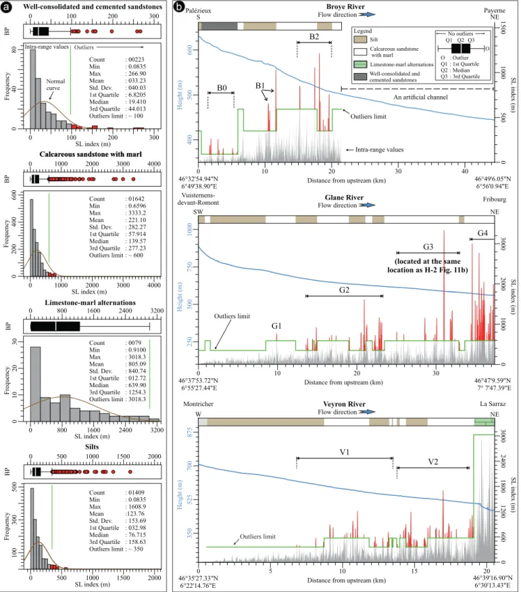
and maximum altitudes on the upstream side (southern side) of the river (Fig. 8a). Although the mean and maximum altitude curves show roughly the same rate of change (increase or decrease) along the entire strip,five distinct positive topographic anomalies can be recognized (labelled B0–B4,Fig. 8a). Fluvial incision variations in a given swath can be indicated by the standard deviation (e.g.,Riquelme et al., 2002), which is the most robust measure of these variations (Evans, 1998). Thus the highest rate offluvial incision is observed between profile distances of ~12 to ~25 km (Fig. 8a).

The analysis of longitudinal profile shows three main SL anomalies (B0, B1and B2 inFig. 8b), which show a direct correlation with the location of the topographic anomalies (B0, B1and B2 inFig. 8a). The highest value of SL (~1300 m) is observed at profile distance ~11.5 km

(Fig. 8a). From the middle toward the end of the profile (distance >

21 km,Fig. 8b), the river was channelized and regulated which was not considered here in terms of the SL assessment.

0.5 Hypsometric Skewness 2 1.5 1 0 0.1 0.2 0.3 0.4 0.5 0.6 0.7 2 3 4 5 6 7 St‒7 St‒9 St‒13a St‒1 St‒2 St‒3 St‒4 St‒5 St‒6 St‒8 St‒10 St‒1 1 St‒13b St‒14 St‒15 St‒16a St‒16b St‒17 St‒2 St‒3 St‒4 St‒5 St‒6 St‒7 St‒8 St‒9 St‒10 St‒1 1 St‒13a St‒13b St‒14 St‒15 St‒16b St‒16a St‒17 St‒12a St‒12b St‒12a St‒12b St‒12 St‒12 St‒1 Hypsometric Kurtosis

Time/Evolution

Less eroded landscape

Significantly eroded landscape

Hypsometric Integral

_Skewness

_{vs. Integral}

Kurtosis vs. Integral

Fig. 4. A graph showing hypsometric integral as a function of the hypsometric kurtosis and skewness values. In general, the hypsometric integral decrease when the skewness and kurtosis values becomes larger. Based on this graph, twenty-one different styles of hypsometric curves can be distinguished. Each style is indicated by a symbol“St” with a number on the graph. In each style, dot and cross symbols with the same color accurately represents one drainage catchment. Colored dots represent hypsometric integral versus hypsometric kurtosis values while colored crossmark represents hypsometric integral versus hypsometric skewness values. (For interpretation of the references to color in thisfigure legend, the reader is referred to the web version of this article.)

(caption on next page)

Fig. 5. Hypsometric curves for seventy-four catchments located in the westernmost part of Switzerland. (a) Twenty-one different shapes of hypsometric curves discriminated based on the relationships between the values of hypsometric integral, skewness and kurtosis (Fig. 4). The area under these curves portrays the volume of material left after erosion (Strahler, 1952). The shapes of these curves are diversified, mostly convex up, S-shaped, and extremely concave up. Catchment no. 62 of the style 1 has the highest value of the hypsometric integral relative to the rest of the data set with a convex-up curve, reflecting a significant amount of land material still existed at high altitude. Whereas catchment no. 56 of the style 17 has the lowest values of the hypsometric integral with the most concave-up curve, indicating that a significant amount of catchment's materials has been removed. (b) Catchment-scale distribution of the hypsometric integral in the westernmost part of Switzerland. The numbers identify each catchment.

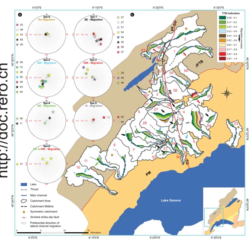
Fig. 6. Mean vectors of TTSI (Transverse Topography Symmetry Index) for the drainage catchments of the westernmost part of the Switzerland (Domain-I). (a) Polar plots (equal-area, lower hemisphere) showing the preferred direction of the principal channel migration in each catchment. Set-0 (TTSI magnitudes≈ 0) indicates there is no preferred direction of the principal channel migration (symmetric catchments). The principal channels of the most catchments have migrated uniformly toward SE and SW directions, set-1 and set-2 respectively. Keys for polar plot are the same as those in Fig. S.4b. (b) Map showing color coded distribution of TTSI magnitude values. Anomalous zone with dark red color (TTSI magnitude≈ 1) implying that stream flowing nearby the catchment margin, whereas those of dark green (TTSI magnitude≈ 0) indicating that stream flowing nearby the catchment midline. TTSI analysis are not applied to the catchments no. 58, 60 and 61 because they have no clear principal channels, but rather several drainage tributariesflowing into their outlets. PF: Pontarlier Fault; JFTB: Jura fold-thrust belt; PM: Plateau Molasse. (For interpretation of the references to color in thisfigure legend, the reader is referred to the web version of this article.)

A distinct change in the curves of the gravityfilters and horizontal gradients of magnetic data at profile distances between ~5 to ~20 km

(Fig. 8c and d) occurs in approximately the same positions of the

aforementioned anomalies, B1 and B2 (Fig. 8a and b). Pre-Cenozoic rocks beneath this river, which are relatively deformed and dip down to the south, occur at a significant depth (Fig. 8e) and are buried beneath the thick Cenozoic sedimentary rocks (Gruber, 2017). In general, to-ward the south in upstream direction (a distance < 20 km), there is a clear increase in the Cenozoic thickness (Fig. 8e) as well as in the re-sidual magnetic gradients (black curve,Fig. 8d).

The Glane river extends about 37 km from its confluent (Neirigue stream) in the southeast, near the town of Vuisternens-devant-Romont, to its outlet into the Sarine river (Supplementary Fig. S.6). The swath topographic profile (Supplementary Fig. S.6a) shows that the maximum and average altitude curves are changing at nearly the same rate, and

reveals several pronounced positive relief zones (labelled by G0, G1, G2, G3, and G4, Fig. S.6a). The highest values of standard deviation (highest rates of incision) are observed in three zones namely, G1, G3, and G4, where the differences between maximum and minimum alti-tudes are highest. The highest SL gradients are noted at two zones (G3 and G4, Fig. S.6b). Small, but noticeable, changes in thefirst vertical gradients of the Bouguer gravity at a profile distance < 12 km (Fig. S.6c) are noted in the same place of the previously determined anomalies, namely G0 and G1 zones (Figs. S.6a and S.6b). Relatively high residual Bouguer values were observed between profile distances 27–34 km (G3, Fig. S.6c), where the residual magnetic gradients are gradually increasing (Fig. S.6d) and the thickness of Cenozoic rock is relatively decreasing (Fig. S.6e). A dramatic decrease in residual mag-netic values (Fig. S.6d) is observed at profile distance < 6 km, and co-incides with a decrease in the altitude of the bottom of the river channel Fig. 7. Mean vectors of TTSI (Transverse Topography Symmetry Index) for the drainage catchments of the westernmost part of the Switzerland (Domain-II). (a) Polar plots (equalarea, lower hemisphere) showing the preferred direction of the principal channel migration in each catchment. Set-0 (TTSI magnitudes≈ 0) indicates there is no preferred direction of the principal channel migration (symmetric catchments). Most of the catchments showing a significant migration for their principal channels toward SE and NW directions (set-1 and set- 2, respectively). Keys for polar plot are the same as those in Fig. S.4b. (b) Map showing color-coded distribution of TTSI magnitude values. Anomalous zone with dark red color (TTSI magnitude≈ 1) implying that stream flowing nearby the catchment margin, whereas those of dark green (TTSI magnitude≈ 0) indicating that stream flowing nearby the catchment midline. JFTB: Jura fold-thrust belt; PA: Prealps; PM: Plateau Molasse; SM: Subalpine Molasse. (For interpretation of the references to color in thisfigure legend, the reader is referred to the web version of this article.)

0 400 800 1200 1600 10 20 30 40 0

Distance from upstream (km) 46°32'54.94"N 6°49'38.90"E 46°49'6.05"N 6°56'0.94"E 300 400 500 600 Height (m) Palézieux Payerne S NE Flow direction Longitudinal river profile

SL Index (m) Channelized river B1 B2 B0

Segment was not considered

b

Distance from upstream (km)

10 20 30 40

First vertical derivative

Horizontal gradient

Residual Bouguer anomaly

T

otal gradient

Palézieux Payerne

S Flow direction NE

Bouguer gravity anomaly (mGal)

0.0004 0.0008 0.0012 0.0016 -12 -8 -4 0 -0.001 0 0.001 -0.0005 0 0.0005 0.001 46°32'54.94"N 6°49'38.90"E 46°49'6.05"N 6°56'0.94"E B1 B2& B0

c

First vertical derivative

Horizontal gradient

Distance from upstream (km)

10 20 30 40 46°32'54.94"N 6°49'38.90"E 46°49'6.05"N 6°56'0.94"E Palézieux Payerne S Flow direction NE

Total-field Aeromagnetic intensity anomaly (nT)

Aeromagnetic residual anomaly

T otal gradient B1 B2& B0

d

Distance from upstream (km)

10 20 30 40 46°32'54.94"N 6°49'38.90"E 46°49'6.05"N 6°56'0.94"E 0 0 Standard deviation T opographic relief (m) Palézieux Payerne S NE Flow direction Topographic swath profile

Maximum altitude Minimum altitude Mean altitude B4 B3 B1 B2 B0

a

2D geologic cross section

400 500 600 10 20 30 40 Cenozoic Cretaceous Upper Malm Lower Malm Dogger Liassic Upper Triassic Lower Triassic Pre-Mesozoic Depth (m) VMF -4000 -3000 -2000 -1000 0 0 -4000 -3000 -2000 -1000 Depth (m)

Distance from upstream (km)

10 20 30 40 46°32'54.94"N 6°49'38.90"E 46°49'6.05"N 6°56'0.94"E

e

Fig. 8. Topographical, geophysical, and longitudinal profiles of the entire 44.5-km length of the Broye river in the westernmost of Switzerland. (a) One-km wide swath profile showing a conspicuous relief approximately on the middle part of river (zones B2 and B3). Maximum and mean altitude curves nearly follow the same pattern of change. (b) Longitudinal profile based on the channel's bottom elevation and gradient (SL index). SL index clearly displays three prominent breaks, labelled by B0, B1, and B2. (c) and (d) Unfiltered and filtered residual gravity and aeromagnetic anomaly profiles along the river path, respectively. (e) Geological cross-section along the river, extracted from a 3D geological model based on the interpretation of seismic reflection data (Gruber, 2017), showing a significant decrease in the thickness of Cenozoic rocks from being ~3000 m at the upper section of river to < 1200 m near the river mouth. Black and red colored lines represent different types of faults interpreted byGruber (2017)andMeier (2010), respectively. FATF: Frontal Alpine thrust fault; LaF: La-Lance strike-slip fault; VMF: Vuacherens-Moudon fault. (For interpretation of the references to color in thisfigure legend, the reader is referred to the web version of this article.)

(Fig. S.6e). The geologic cross section along the river consists of ~2000 to ~2800 m thick Cenozoic sediments covering layers of Mesozoic age (Supplementary Fig. S.6e). Alternate patterns of high and low residual Bouguer values characterize the profile along the river (Fig. S.6c) and are relatively parallel to the subsurface geometry of the Mesozoic strata (Fig. S.6e).

The studied part of the Veyron river extends 20.56 km from its confluent (Malagne stream) in the west, near the town of Montricher, to the northeast in the vicinity of the town of la Sarraz (Supplementary Fig. S.7). Its swath profile shows three distinct topographic anomalies, located in the upper, central and lower parts of the profile (V0, V1 and V2, Fig. S.7a). The lower part of the profile, however, shows the highest rate of incision, as the standard deviation reaches 20 (Fig. S.7a). Two pronounced SL anomaly zones can be identified in the central and lower parts of the river course (V1 and V2, Fig. S.7b). The most prominent one (V2 Fig. S.7b) is characterized by a sharp break in the elevation curve with the highest SL value (~3000 m). A conspicuous change in thefilter curves of the gravity and magnetic at the central part of the profile (~6 - ~14 km, Figs. S.7c and S.7d) is noted at the same location of the zone V1 (Figs. S.7a and S.7b). Cretaceous rocks under the studied part of the river course, occur at shallow depth and crop out in a small portion at the upper and lower section of the river course (Fig. S.7e).

5. Discussion

We discuss the results of GIS-based quantitative geomorphic ana-lysis and the level of evidence they provide to highlight the effects of tectonic deformation on the development of fluvial landscape in the westernmost part of Switzerland.

5.1. Tectonic controls on hypsometry

The results achieved by considering interrelationships among hyp-sometric attributes (integral, skewness and kurtosis), presented as graph (Fig. 4), clearly highlight the importance of the hypsometric at-tributes for classification and characterization of landscape evolution patterns. According to these attributes, significant differences in the shape of the hypsometric curves, and thus fluvial landscapes, were observed (Fig. 5a), that cannot be fully noticed with the integral values alone. These variations reflect a relatively high level of evolutionary diversity in the study area that is usually attributed to the isolated or combined impacts of tectonic uplift, lithology, and glacial erosion (e.g.,

Hurtrez and Lucazeau, 1999;Lifton and Chase, 1992;Schlunegger and

Norton, 2013;Sternai et al., 2011;Stutenbecker et al., 2016).

Knowledge about the effects of the lithology and glacial erosion is therefore essential for evaluating tectonic role. The lithology effect was statistically segregated (Fig. 9) using a special filter, described in

Section 3.2.4. According to the composition of the host lithology, the

hypsometric integral values were classified into four different groups. Summary statistics for each group are separately shown inFig. 9a. Al-though there are some anomalous observations, the hypsometric in-tegral values in all the classes are roughly clustered around their mean values of ~0.5 and follow quite closely a normal distribution, in-dicating that the lithology exerted an important influence on the dis-tribution of hypsometric integral values. The anomalous observations, which have unusually high and low hypsometric integral values, are sparse and irregularly distributed in the study area (labelled H-1, H-2, H-3, and L inFig. 9b). These abnormalities can't be explained as being the results of variation in lithology, but rather as the results of glacial erosion or tectonic processes. The Alpine glacier at the last glacial maximum had significantly influenced the landscape evolution of the Swiss Alps and the northern Alpine foreland (e.g.,Norton et al., 2010a;

Salcher et al., 2014;Schlunegger and Norton, 2013;Stutenbecker et al.,

2016;Valla et al., 2011;van Der Beek and Bourbon, 2007). It left

be-hind unique topographical imprints, which are noticeably different from those achieved byfluvial erosion process, such as hanging valleys,

moraine ridges, glacial cirques, and glacially polished rocks (e.g.,Fiebig

and Preusser, 2008;Ivy-Ochs et al., 2006; Kelly et al., 2004;Wirsig

et al., 2016). Several studies have shown that the last glacial maximum

deglaciation associated with an isostatic crustal rebound of the Alpine region (Gudmundsson, 1994;Mey et al., 2016). This implies that the isostatic rebound cannot be ruled out as partly or largely responsible for the elevation differences in the study area. However, it is not possible here to differentiate between the impacts of post-glacial isostatic ad-justment and tectonic processes.

The extent of the Alpine glacier at the last glacial maximum in the Swiss Alps and in the northern Alpine foreland (around 24,000 years ago) was reconstructed by a group of researchers (e.g.,Florineth, 1998;

Florineth and Schlüchter, 1998; Kelly et al., 2004), which was then

updated in a recent map covering the entire Switzerland by (Bini et al., 2009). This map (Fig. 9c) displays almost none or very limited influence

of ice on the areas where the unusually high values of hypsometric integral (H-1 and H-3) are developed, and therefore the latter can be directly attributed to tectonic activity. In this context, we interpreted anomaly H-1 (Fig. 9b) as a result from the growth of the anticlines in response to slip movements along thrust faults. This agrees with our hypothesis that thrust-related fold growth creates a local relief, which is then eroded by rivers incision. The H-3 anomaly (Fig. 9b) occurs on the hanging wall of the Frontal Alpine thrust fault system, suggesting that the tectonic movement along Frontal Alpine thrust fault system is most probably responsible for increasing the hypsometric integral values.

Conversely, high values of hypsometric integral (H-2) occur in the area that was covered by a ~1 km thick ice sheet (Fig. 9b and c), where glacial erosional features were identified using the Swisstopo LiDAR data. Thick glaciers that have high ice discharges often induce a sig-nificant landscape modification through increasing the amount and intensity of glacial erosion and consequently a reduction in the value of hypsometry (Brocklehurst and Whipple, 2004). This suggests that the anomaly H-2 is not caused by the glacial erosion but by tectonic effects. Comparison of the location of anomaly H-2 with subsurface tectonic map suggests (Fig. 9b) that it is caused by reactivation of pre-existing thrust fault. The unusually low values of the hypsometric integral (L in

Fig. 9b), which are roughly developed in the same locations of paleo-ice

stream pathways, where the depth to bedrock increases, are most probably due to the intensive glacial erosion. Variations in bedrock surface elevation beneath the Quaternary cover can provide essential information for the identification of erosional processes during past glaciations (Dürst-Stucki and Schlunegger, 2013). However, hypso-metric technique alone cannot offer conclusive evidence on the process that is responsible for the land surface modifications because many processes can have very similar imprints on the topography.

5.2. Tectonic controls on the lateral channel migration

Ourfindings obtained from the analysis of TTSI indicate that most of the studied catchments of the study area are asymmetric and char-acterized by uniform patterns of lateral channel migration (Figs. 6 and 7). Remarkably, both the domains show a great similarity in the pre-vailing directions of channel migration toward SE and NW (sets-1&-3 of

Fig. 6a and sets-1&-2 ofFig. 7a). They differ, however, in the presence

of other main trends of channel migration toward SW within the do-main-I (sets-2,Fig. 6a) and toward ~W and ~E within the domain-II (sets-3&-4 ofFig. 7a). Growing body of research demonstrates that the lateral migration of river would be useful to infer the direction of tec-tonic tilting if the other influencing factors, e.g., lithology and glacial erosion, remain neutral (Alves et al., 2018;Cox, 1994;Cox et al., 2001;

Ibanez et al., 2014;Salvany, 2004). Thus, a common problem that faces

us is to discriminate between channel migrations driven by tectonics or by the lithological variations and glacial erosion. The abundant pre-sence of glacial erosional features, such as roches moutonées and drumlins, in many parts of the study area makes it extremely difficult to differentiate between the influence of glacial and tectonic processes.

Furthermore, the effect of lithology can't be neglected, especially in many drainage catchments, where the spatial variations in their un-derlying rock properties appear to be non-uniform (e.g., catchment no. 41, 42, 43, and 45 Fig. 10a).Despite the difficulties in assessing the impacts of lithological variations and glacial erosion on the fluvial landscapes, most of the bedding planes within both domains are slightly dipping toward SE and NW directions (Fig. 10b and c). The latter are in agreement with the dominant directions of channel migration shown in

Fig. 6a (sets-1&-3) andFig. 7a (sets-1&-2). This fact generally supports findings from previous studies (Chittenden et al., 2013;Nunes et al., 2015) that imply that landscape properties in many basins within the Central European Alps are highly controlled by the tectonic architecture of the underlying bedrock. It could also support our hypothesis that tectonic processes have caused lateral tilting of the ground surface in a

direction parallel to the direction of maximum compressive stress. Such behaviour of lateral ground tilting dates back to any time after the beginning of deformation in the Jura Mountains and Molasse Basin (Miocene time).

5.3. Fault-induced uplift, stream migration and deflection

Possible tectonic control can be observed in the drainage system located in the vicinity of known structures. Afirst example is given by the catchments (no. 23, 26, 35, 44, 67, 68, 69, 71, 72 and 74,Fig. 11a) that are located immediately in the south (hanging wall) and north (footwall) sides of Frontal Alpine thrust fault system. The catchments (no. 35, 44, 69, 71, and 74) located immediately in the hanging wall of the Frontal Alpine thrust fault display SE to S directed migration for Fig. 9. Hypsometric integral values versus lithology and ice thickness distribution. a) Box plots and frequency histograms (lithological-filtering) showing the normal and abnormal values of the hypsometric integral for each host rock lithology. Most of the hypsometric integral values in all lithological units are roughly clustered around their mean values of ~0.5, highlighting the significant impact of lithology on the hypsometry. b) Spatial distribution of abnormal hypsometric integral values (labelled H-1, H-2, H-3, and L), superimposed on a simplified sub/surface tectonic elements of the westernmost of Switzerland. c) Ice thickness distribution during the last glacial maximum (LGM, 24,000 years ago) covered large parts of the study area (Bini et al., 2009). Unusually high values of the hypsometric integral (1and H-3) are shown to be related to the hanging walls of the thrust faults, while unusually low values (L) are shown to be related to glacial erosion.