researchers and makes it freely available over the web where possible
This is a Publisher’s version published in:
http://oatao.univ-toulouse.fr/24125
To cite this version:
Tachella, Julian and Altmann, Yoann and Ren, Ximin and McCarthy, Aongus
and Buller, Gerald S. and Mclaughlin, Stephen and Tourneret, Jean-Yves
Bayesian 3D Reconstruction of Complex Scenes from Single-Photon Lidar Data.
(2019) SIAM Journal on Imaging Sciences, 12 (1). 521-550. ISSN 1936-4954
Official URL:
https://doi.org/10.1137/18M1183972
Abstract. Light detection and ranging (Lidar) data can be used to capture the depth and intensity profile of a 3D scene. This modality relies on constructing, for each pixel, a histogram of time delays between emitted light pulses and detected photon arrivals. In a general setting, more than one surface can be observed in a single pixel. The problem of estimating the number of surfaces, their reflectivity, and position becomes very challenging in the low-photon regime (which equates to short acquisition times) or relatively high background levels (i.e., strong ambient illumination). This paper presents a new approach to 3D reconstruction using single-photon, single-wavelength Lidar data, which is capable of identifying multiple surfaces in each pixel. Adopting a Bayesian approach, the 3D structure to be recovered is modelled as a marked point process, and reversible jump Markov chain Monte Carlo (RJ-MCMC) moves are proposed to sample the posterior distribution of interest. In order to promote spatial correlation between points belonging to the same surface, we propose a prior that combines an area interaction process and a Strauss process. New RJ-MCMC dilation and erosion updates are presented to achieve an efficient exploration of the configuration space. To further reduce the computational load, we adopt a multiresolution approach, processing the data from a coarse to the finest scale. The experiments performed with synthetic and real data show that the algorithm obtains better reconstructions than other recently published optimization algorithms for lower execution times.
Key words. Bayesian inference, 3D reconstruction, Lidar, low-photon imaging, Poisson noise AMS subject classifications. 62F15, 62H12, 62H35, 62P30, 62P12, 65C40
DOI. 10.1137/18M1183972
1. Introduction. Reconstruction and analysis of 3D scenes have a variety of applications,
spanning earth monitoring [16,35,28], underwater imaging [27,18], automotive [36,41], and
defense [14]. Single-photon light detection and ranging devices acquire range measurements
by illuminating a 3D scene with a train of laser pulses and recording the time-of-flight (TOF)
\ast
Received by the editors April 30, 2018; accepted for publication (in revised form) December 27, 2018; published electronically March 14, 2019. The codes used in this paper are available online at https://gitlab.com/tachella/ manipop.
http://www.siam.org/journals/siims/12-1/M118397.html
Funding: The work of the first and sixth authors was supported by the UK Quantum Technology Hub in Quantum Enhanced Imaging (QuantIC). The work of the second author was supported by the Royal Academy of Engineering via the Research Fellowship Scheme (RF201617/16/31). The work of the sixth author was supported by the UK Engineering and Physical Sciences Research Council (EPSRC), grants EP/N003446/1, EP/M01326X/1, EP/K015338/1. The work of the seventh author was partly conducted within the ECOS project ``Colored apertude design for compressive spectral imaging"" supported by CNRS and Colciencias, and within the STIC-AmSud Project HyperMed.
\dagger
School of Engineering and Physical Sciences, Heriot-Watt University, Edinburgh, EH14 4AS, UK ([email protected],
https://tachella.github.io;[email protected];[email protected];[email protected];[email protected];
\ddagger
INP-ENSEEHIT-IRIT-TeSA, University of Toulouse, 31071 Toulouse Cedex 7, France (Jean-Yves.Tourneret@ enseeiht.fr).
of the photons reflected from the objects in the illuminated scene. Using a time correlated single-photon counting (TCSPC) system, a histogram of time delays between emitted and reflected pulses is constructed for each pixel. For a given pixel, the presence of an object is associated with a characteristic distribution of photon counts in the histogram. The position and number of counts provide depth and reflectivity information, respectively. In scenarios where the light goes through a semitransparent material (e.g., windows or camouflage) or when the laser beam is wide enough with respect to the object size (e.g., distant objects), it is possible to record two or more surfaces in a single pixel. The recovery of multiple objects per
pixel is thus very important in many applications, such as tree layer analysis [48] or detection
of hidden targets behind camouflage [19].
In order to reconstruct the 3D scene from single-photon Lidar data, it is necessary to discriminate the photon counts associated with each surface from the ones linked to the back-ground illumination. When the backback-ground level can be neglected, the traditional approach consists, under the single-peak assumption, of log-match filtering the Lidar waveforms and
finding the maximum of the filtered data for each pixel [44], which is the maximum likelihood
(ML) solution for a Poisson noise assumption (a matched filter is used for Gaussian noise). While this method obtains good results for high photon counts, it gives poor estimates when the background illumination is high or the number of recorded photons is low. Several studies have focused on improving the ML estimates in the single-depth estimation problem. Altmann
et al. [5] proposed a Bayesian approach, whereas Shin et al. [42], Halimi et al. [17], and Rapp
and Goyal [38] suggested three different optimization alternatives. The method introduced in
[42] estimates the reflectivity and depth information independently, considering a rank-ordered
mean censoring of background photons as a preprocessing step. The optimization method in
[17] assumes a negligible background and estimates the depth and reflectivity jointly using an
alternating direction method of multipliers (ADMM) algorithm. The algorithm proposed in
[38] uses an adaptive superpixel approach to censor background photons and improve depth
and reflectivity estimates. In the multiple-surface-per-pixel configuration, Hernandez-Marin,
Wallace, and Gibson [23] proposed a pixelwise reversible jump Markov chain Monte Carlo
(RJ-MCMC) algorithm. While this approach is able to find an a priori unknown number of surfaces and compute associated uncertainty intervals, it involves a prohibitive computation time. Moreover, it performs poorly when photon counts are relatively low, as it does not account for spatial correlation between neighboring pixels. In later work, Hernandez-Marin,
Wallace, and Gibson [24] proposed an extension to the latter algorithm, where a Potts model
was used to regularize spatially the number of surfaces per pixel. However, the computational load of their algorithm was prohibitive for large images and the correlation between the am-plitude and position of each object was not modelled a priori. There have been other attempts to derive statistical models for Lidar waveforms with an unknown number of objects per pixel,
such as Mallet et al. [29] with full waveform topographic Lidar, where a marked point process
was considered for each pixel separately. While they defined interactions between pulses in the same pixel, no spatial interaction between points of neighboring pixels was considered. Recently, new optimization approaches have been proposed to tackle the
multiple-object-per-pixel problem: Shin et al. [43] introduced an \ell 1 norm regularization for the recovered peak
positions, followed by a postprocessing of the 3D point cloud. Halimi et al. [19] improved it
(a) (b) 0 1000 2000 3000 4000 Histogram bin 0 0.1 0.2 0.3 Poisson intensity pixel (59,63) pixel (47,73) pixel (41,61) (c) 0 1000 2000 3000 4000 Histogram bin 0 0.5 1 1.5 2
Observed photon counts Poisson intensity
(d)
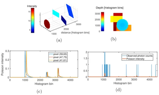
Figure 1. (a) depicts a synthetic 3D point cloud with Nr = 99 rows, Nc = 99 columns, and T = 4500
bins. The scene consists of three plates with different sizes and orientations and one ball-shaped object. The intensity represents the mean number of photons associated with each 3D point. (b) illustrates the depth of the first object for each pixel. (c) shows the intensity of three different pixels. The observed photon counts and underlying Poisson intensity of a pixel with three surfaces are shown in (d).
In this work, we introduce a new spatial point process within a Bayesian framework for modelling single-photon Lidar data. This novel approach considers interactions between points at a pixel level and also at an interpixel level, in a variable dimension configuration. Here, we consider each surface within a pixel as a point in the 3D space, which has a mark that indicates its intensity. Natural Lidar point clouds exhibit strong spatial clustering, as points belonging to the same surface tend to be close in range. Conversely, points in a given pixel
tend to be separated as they correspond to different surfaces. Figure 1 shows an example
of a synthetic Lidar 3D point cloud to illustrate this phenomenon. This prior information is added to our model using spatial point processes: repulsion between points at a pixel level is achieved with a hard constraint Strauss process, and attraction among points in neighboring
pixels is attained by an area interaction process, as defined in [47]. Moreover, the combination
of these two processes implicitly defines a connected-surface structure that is used to efficiently sample the posterior distribution. To promote smoothness between reflectivities of points in the same surface, we define a nearest neighbor Gaussian Markov random field (GMRF) prior
model, similar to the one proposed in [31]. Inference about the posterior distribution of points,
their marks, and the background level is done by an RJ-MCMC algorithm [10, Chapter 9],
with carefully tailored moves to obtain high acceptance rates, ensuring better mixing and faster convergence rate. In addition to traditional birth/death, split/merge, shift, and mark moves, new dilation/erosion moves are introduced, which add and remove new points by extending or shrinking a connected surface, respectively. These moves lead to a much higher acceptance rate than those obtained for birth and death updates, as they propose moves to and within regions of high posterior probability. To further reduce the transient regime
of the Markov chains and reduce the computational time of the algorithm, we consider a multiresolution approach, where the original Lidar 3D data is binned into a coarser resolution data cube with higher signal power, lower number of points, and same data statistics. An initial estimate obtained from the downsampled data is used as the initial configuration for the finer scale, thus reducing the number of burn-in iterations needed for the Markov chains to convergence. We assess the quality of reconstruction and the computational complexity in several experiments based on synthetic Lidar data and three real Lidar datasets. The algorithm leads to new efficient 3D reconstructions with processing times similar to those of other existing optimization-based methods. This method can be successfully applied to scenes where there is only one object per pixel, thus generalizing other single-depth algorithms
[42, 5, 19, 38]. Moreover, the proposed algorithm can also be applied in scenes where each
pixel has at most one surface and it generalizes other target detection methods [6]. We refer
to the proposed method as ManiPoP, as it aims to represent 2D manifolds with a 3D point process. In summary, the main contributions of this paper are
1. a new Bayesian model based on a marked point process prior for modelling spatially correlated 3D point clouds,
2. new reversible jump moves proposed for sampling the posterior distribution more efficiently,
3. a multiresolution processing approach to improve the convergence rate, which also allows for a rapid information extraction using only the coarser scales.
The remainder of this work is organized as follows. Section 2 presents the Bayesian
model considered for the analysis of multiple-depth Lidar data. Section 3details the sampling
strategy using an RJ-MCMC algorithm. Section 4 discusses the proposed multiresolution
approach and other implementation details to reduce the computational load of the algorithm.
Results of experiments conducted on synthetic and real data are presented insection 5. Finally,
section 6summarizes our conclusions and discusses future work.
2. Proposed Bayesian model. Recovering the position and intensity of the objects from
the raw Lidar data is an ill-posed problem, as the solution is not uniquely identified given the
data (e.g., the histogram ofFigure 1d). This problem can be tackled in a Bayesian framework,
where the data generation mechanism is modelled through a set of parameters \bfittheta that can be inferred using the available data \bfitZ . The probability of observing a Lidar cube \bfitZ is given by the likelihood p(\bfitZ | \bfittheta ). The a priori knowledge of the unknown parameters \bfittheta is embedded in the prior distribution p(\bfittheta | \Psi ) given a set of hyperparameters \Psi . Following Bayes' theorem, the posterior distribution of the model parameters is
(2.1) p(\bfittheta | \bfitZ , \Psi ) = p(\bfitZ | \bfittheta )p(\bfittheta | \Psi )
\int p(\bfitZ | \bfittheta )p(\bfittheta | \Psi )d\bfittheta .
2.1. Likelihood. A 3D point cloud is represented by an unordered set of points
bin t and pixel (i, j) follows a Poisson distribution, whose intensity is a mixture of the pixel
background level bi,j and the responses of the surfaces present in that pixel, i.e.,
(2.3) zi,j,t| (\Phi , bi,j) \sim \scrP
\left(
\sum
n:(xn,yn)=(i,j)
gi,jrnh(t - tn) + gi,jbi,j
\right) ,
where t \in \{ 1, . . . , T \} , T is the number of histogram bins, h(\cdot ) is the known temporal
instru-mental response, and gi,j is a scaling factor that represents the gain/sensitivity of the detector
in pixel (i, j). Assuming mutual independence between the noise realizations in different time bins and pixels, the full likelihood can be written as
(2.4) p(\bfitZ | \Phi , \bfitB ) =
Nc \prod i=1 Nr \prod j=1 T \prod t=1
p(zi,j,t| \Phi , bi,j),
where \bfitZ is the full Lidar cube with [\bfitZ ]i,j,t = zi,j,t, \bfitB is the background 2D image, and Nr
and Nc are the numbers of pixels in the vertical and horizontal axes, respectively. Note that
p(zi,j,t| \Phi , bi,j) in (2.4)is the Poisson distribution associated with(2.3).
2.2. Markov marked point process. The set of points \Phi is defined inside the 3D space
\scrT = [0, Nr] \times [0, Nc] \times [0, T ]. Interactions between points can be characterized by defining
densities with respect to the Poisson reference measure, i.e.,
f (\Phi c) \propto f1(\Phi c) . . . fr(\Phi c),
where \propto means ``proportional to."" A more detailed definition of the point process theory can
be found in section SM1. In this work, we only consider Markovian interactions between
points. The benefits of this property are twofold: (a) Markovian interactions are well suited
to describe the spatial correlations in natural 3D scenes [32] and (b) inference is performed
using only local updates, which leads to a low computational complexity. We can constrain the minimum distance between two different surfaces in the same pixel using the hard object process with density
(2.5) f1(\Phi c) \propto
\left\{
0 if \exists n \not = n\prime : xn= xn\prime , yn= yn\prime ,
and | tn - tn\prime | < d\mathrm{m}\mathrm{i}\mathrm{n},
1 otherwise,
which is a special case of the repulsive Strauss process [47], where d\mathrm{m}\mathrm{i}\mathrm{n} is the minimum
distance between two points in the same pixel. Attraction between points of the same surface in
1
The reflectivity of the point, limited to (0, 1], can be obtained as max\{ 1, rn/(\eta N\mathrm{r}\mathrm{e}\mathrm{p}\sum th(t))\} , where
neighboring pixels cannot be modelled with another Strauss process, due to a phase transition
of extremely clustered realizations, as explained in [47, 32]. However, a smoother transition
into clustered configurations can be achieved by the area interaction process, introduced by
Baddeley and van Lieshout in [8]. In this case, the density is defined as
(2.6) f2(\Phi c| \gamma a, \lambda a) = k1\lambda Na\Phi \gamma
- m\Bigl( \bigcup N\Phi
n=1S(\bfitc n)
\Bigr)
a ,
where \lambda ais a positive parameter that controls the total number of points, \gamma a\geq 1 is a parameter
adjusting the attraction between points, and k1 is an intractable normalizing constant. The
exponent of \gamma a in(2.6)is the measure m(\cdot ) over the union of convex sets S(\bfitc n) \subseteq \scrT centered
around each point \bfitc n. In this way, the density is bigger when the intersection of the convex
sets around two interacting points is closer to the union of them, i.e., if the points are clustered
together. The special case \gamma a= 1 corresponds to a Poisson point process (without considering
a Strauss process) with an intensity proportional to \lambda a\lambda (\cdot ) (see section SM2for details). In
the rest of this work, we fix \lambda (\scrT ) = 1 and control the number of points with the parameter
\lambda a. The set S(\bfitc n) is defined as a cuboid with a face of Np\times Np squared pixels and a depth
of 2Nb + 1 histogram bins, and m(\cdot ) is the Lebesgue measure on \scrT . This set determines a
cuboid of influence around each point, allowing interactions up to a distance of \lfloor Np/2\rfloor pixels
and Nb bins. As two points in the same pixel generally correspond to different surfaces, we set
d\mathrm{m}\mathrm{i}\mathrm{n}> 2Nb, thus constraining the minimum distance between two surfaces in the same pixel.
The combination of the Strauss process and the area interaction process implicitly defines a connected-surface structure.
(a) (b) (c)
Figure 2. (a) and (b) show two different point configurations. Each point \bfitc nis denoted by a black dot, and
the corresponding blue rectangle depicts the area of the convex set S(\bfitc n). The configuration shown in (a) has a
lower prior probability than the one shown in (b), as the union of all sets S(\bfitc n) is smaller in (b) with respect
to the Lebesgue measure. (c) shows the connectivity at an interpixel level when Np= 3. The green and blue
squares correspond to pixels with points associated with two different surfaces, while the white squares denote pixels without points. For simplicity, in this example all points are considered to be present at the same depth. Note that each pixel can be connected with at most eight neighbors.
Figures 2 and 3 illustrate the connected-surface structure via several examples. The
hyperparameters \gamma a and \lambda a of the area interaction process are difficult to estimate, as there
is an intractable normalizing constant in the density of (2.6)and standard MCMC methods
cannot be directly applied. Although there exist ways of bypassing this problem (e.g., [33]),
we fixed these hyperparameters in all our experiments to ensure a reasonable computational complexity.
(a) (b)
Figure 3. In both figures, the red color denotes the space where no other points can be found (Strauss process), whereas the blue color denotes the volume where other points are likely to appear (area interaction process with Np = 3). (a) Example of configuration with one point. (b) Example of configuration with three
points.
After defining the spatial priors, the marked point process is constructed by adding the
intensity marks rn to the set \Phi cwith the density detailed in the next section. An illustration
of the proposed prior can be found in section SM4.
2.3. Intensity prior model. In natural scenes, the intensity values of points within the same surface exhibit strong spatial correlation. Following the Bayesian paradigm, this prior knowledge can be integrated into our model by defining a prior distribution over the point marks. Gaussian processes are classically used in spatial statistics. However, the underly-ing covariance structure needs to consider too many neighborunderly-ing points to attain sufficient smoothing, which involves a prohibitive computational load. In order to obtain similar results with a lower computational burden, we propose to exploit the connected-surface structure to define a nearest neighbor Gaussian Markov random field (GMRF), similar to the one used by
McCool et al. in [31]. First, we alleviate the difficulties induced by the positivity constraint
of the intensity values by introducing the following change of variables, which is a standard
choice in spatial statistics dealing with Poisson noise (see [39, Chapter 4]):
(2.7) mn= log(rn), n = 1, . . . , N\Phi c.
Second, spatial correlation is promoted by defining the following conditional distribution of the log-intensities:
(2.8) p(mn| \scrM pp(\bfitc \bfitn ), \sigma 2, \beta ) \propto exp
\left( - 1 2\sigma 2 \left( \sum n\prime \in \scrM pp(\bfitc n) (mn - mn\prime )2
d(\bfitc n; \bfitc n\prime ) + m
2
n\beta
\right) \right)
,
where \scrM pp(\bfitc n) is the set of neighbors of \bfitc n, d(\bfitc n; \bfitc n\prime ) denotes the distance between the points
\bfitc n and \bfitc n\prime , and \beta and \sigma 2 are two positive hyperparameters. The set of neighbors \scrM pp(\bfitc n)
is obtained using the connected-surface structure, where each point can have at most Np2 - 1
neighbors, as illustrated in Figure 2. The distance between two points is computed according
to
d(\bfitc n; \bfitc n\prime ) =
\sqrt{}
(yn - yn\prime )2+ (xn - xn\prime )2+\biggl( tn
- tn\prime
lz
\biggr) 2
with lz = \Delta p/\Delta b, which normalizes the distance to have a physical meaning, where \Delta p and \Delta b
prior promotes a linear interpolation between neighboring2 intensity values, as explained in
[39]. In this work, we assume that \Delta p is constant throughout the scene. If the scene presents
significant distortion, i.e., objects separated by a significant distance in depth, \Delta p should
depend on the position by computing the projective transformation between world
coordi-nates and Lidar coordicoordi-nates (a detailed explanation can be found in [13,22]). Following the
Hammersley--Clifford theorem [20], the joint intensity distribution is given by the multivariate
Gaussian distribution
(2.9) \bfitm | \sigma 2, \beta , \Phi c\sim \scrN (0, \sigma 2\bfitP - 1),
where \bfitP is the unscaled precision matrix of size N\Phi \times N\Phi with the following elements:
(2.10) [\bfitP ]n,n\prime = \left\{ \beta +\sum \~ n\in \scrM pp(\bfitc n) 1 d(\bfitc n;\bfitc n\~) if n = n \prime , - d(\bfitc 1
n;\bfitc n\prime ) if \bfitc n\in \scrM pp(\bfitc n \prime ),
0 otherwise.
The parameter \sigma 2controls the surface intensity smoothness, and \sigma \beta 2 is related to the intensity
variance of a point without any neighbor. In addition, the parameter \beta ensures a proper joint
prior distribution, as \bfitP is diagonally dominant, thus full rank [39].
2.4. Background prior model. Noncoherent illumination sources, such as the solar illu-mination in outdoor scenes or room lights in the indoor case, are related to arrivals of photons at random times (uniformly distributed in time) to the single-photon detector. The level of
these spurious detections is modelled as a 2D image of mean intensities bi,j with i = 1, . . . , Nr
and j = 1, . . . , Nc. If the transceiver system of the Lidar is monostatic3 (e.g., the system
described in [30]), the background image is usually similar to the objects present in the scene
and exhibits spatial correlation, as background photons generally arise from the ambient light reflecting from parts of the targets and being collected by the system. Hence, we use a hidden gamma Markov random field prior distribution for \bfitB that takes into account the background
positivity and spatial correlation. This prior was introduced by Dikmen and Cemgil in [12]
and applied in many image processing applications with Poisson likelihood [2,3]. In [12], the
distribution of bi,j is defined via auxiliary variables [\bfitW ]i,j = wi,j such that
bi,j| \scrM B(bi,j), \alpha B \sim \scrG
\biggl( \alpha B, bi,j \alpha B \biggr) , (2.11)
wi,j| \scrM B(wi,j), \alpha B \sim \scrI \scrG (\alpha B, \alpha Bwi,j),
(2.12)
where \scrM B denotes the set of five neighbors as shown in Figure 4, \scrG and \scrI \scrG indicate gamma
and inverse gamma distributions, \alpha B is a hyperparameter controlling the spatial
regulariza-2
The combination of a local Euclidean distance with a nearest neighbors definition can be seen to approxi-mate the manifold metrics [45].
3
The transceiver system is monostatic when the transmit and receive channels are coaxial and thus share the same objective lens aperture.
(a) (b)
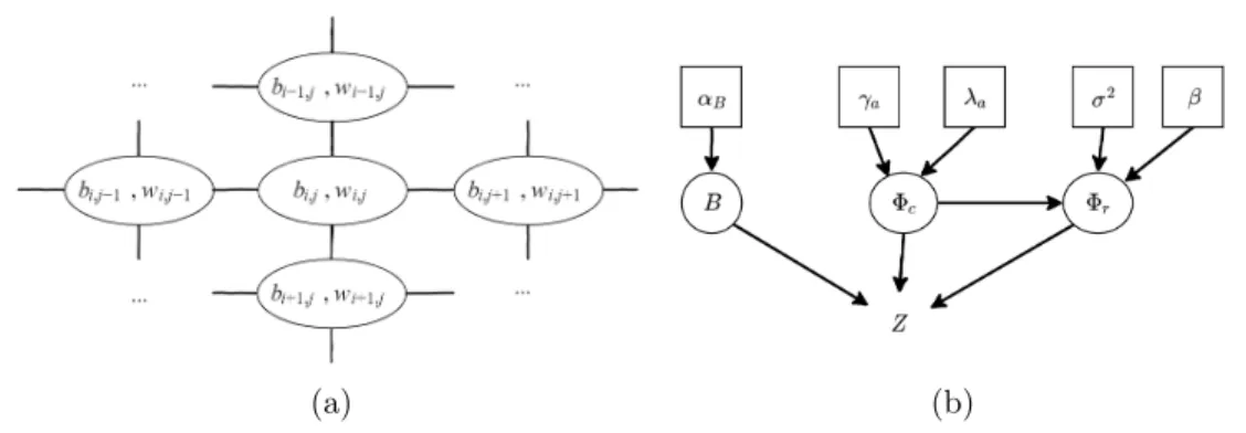
Figure 4. (a) illustrates the gamma Markov random field neighboring structure \scrM B. Each bi,j is connected
to five auxiliary variables wi\prime ,j\prime as depicted by the continuous lines, including the one with the same subscript. Similarly, each wi,jis also connected to five other variables bi\prime ,j\prime as indicated by the continuous lines. (b) shows the directed acyclic graph of the proposed hierarchical Bayesian model. The variables inside squares are fixed, whereas the variables inside circles are estimated.
tion, and bi,j = \left( 1 4 \sum
(i\prime ,j\prime )\in \scrM B(bi,j) w - 1i\prime ,j\prime \right) - 1 , (2.13) wi,j = 1 4 \sum
(i\prime ,j\prime )\in \scrM B(wi,j)
b(i\prime ,j\prime ).
(2.14)
We are interested in the marginal distribution of the GMRF p(\bfitB | \alpha B) that integrates over all
possible realizations of the auxiliary variables wi,j. The expression of this marginal density
can be obtained analytically (as detailed insection SM3) as
p(\bfitB | \alpha B) \propto
\int
p(\bfitB , \bfitW | \alpha B)d\bfitW
(2.15) \propto Nc \prod i=1 Nr \prod j=1 b\alpha B - 1 i,j \Bigl( \sum
(i\prime ,j\prime )\in \scrM
B(wi,j)bi\prime ,j\prime
\Bigr) \alpha B.
(2.16)
In this work, we fix the value of \alpha B, even if it could also be estimated using a stochastic
gradient procedure as explained in [37], at the expense of an increase in the computational
load. If the system is not monostatic, i.e., there is no prior assumption of smoothness in the
background image, the value of \alpha B is set to 1.
2.5. Posterior distribution. The joint posterior distribution of the model parameters is given by
(2.17) p(\Phi c, \Phi r, \bfitB | \bfitZ , \Psi ) \propto p(\bfitZ | \Phi c, \Phi r, \bfitB )p(\Phi r| \Phi c, \sigma 2, \beta )
\times f1(\Phi c| \gamma a, \lambda a)f2(\Phi c| \gamma st)\pi (\Phi c)p(\bfitB | \alpha B),
where \Psi denotes the set of hyperparameters \Psi = \{ \gamma a, \lambda a, \gamma s, \sigma 2, \beta , \alpha B\} . Figure 4 shows the
3. Estimation strategy. Bayesian estimators associated with the full posterior in (2.17)
are analytically intractable. Moreover, standard optimization techniques cannot be applied due to the highly multimodality of the posterior distribution. However, we can obtain numer-ical estimates using samples generated by a Monte Carlo method denoted as
(3.1) \{ \Phi (s), \bfitB (s) \forall s = 0, 1, . . . , Ni - 1\} ,
where Ni is the total number of samples. In this work, we will focus on the maximum a
posteriori (MAP) estimator of the point cloud positions and intensity values, i.e.,
(3.2) \Phi = arg max\^
\bfPhi
p(\Phi , \bfitB | \bfitZ , \Psi ), which is approximated by
(3.3) \Phi \approx arg max\^
s=0,...,Ni - 1
p(\Phi (s), \bfitB (s)| \bfitZ , \Psi ).
In our experiments, we found that the minimum mean squared error estimator of \bfitB , i.e.,
(3.4) \bfitB = \BbbE \{ \bfitB | \bfitZ , \Psi \} ,\^
achieves better background estimates than the MAP estimator. This estimator can be ap-proximated by the empirical mean of the posterior samples of \bfitB , that is,
(3.5) \bfitB \approx \^ 1 Ni Ni \sum s=N\mathrm{b}\mathrm{i}+1 \bfitB (s),
where N\mathrm{b}\mathrm{i} = Ni/2 is the number of burn-in iterations. In many applications, assessing the
presence or absence of a target at a pixel level can be of special interest (e.g., [19,6]). Here,
we can use the Monte Carlo samples to estimate the probability of having k objects present in pixel (i, j) as
(3.6) P (k returns in (i, j)| \bfitZ , \Psi ) = 1
Ni
Ni
\sum
s=N\mathrm{b}\mathrm{i}+1
1k \mathrm{p}\mathrm{o}\mathrm{i}\mathrm{n}\mathrm{t}\mathrm{s} \mathrm{i}\mathrm{n} (i,j)(\Phi (s)).
Remark. If more detailed posterior statistics are needed, it is possible to fix the
dimension-ality of the problem using the estimate \^\Phi and run a fixed dimensional sampler for additional
Ni iterations (seesection SM5).
Many samplers capable of exploring different model dimensions, i.e., different numbers of points, are available in the point process literature (a complete summary can be found in
[10, Chapter 9]). The continuous birth-death chain method builds a continuous-time Markov
chain that converges to the posterior distribution of interest. Alternatively, perfect sampling approaches generate samples using a rejection sampling scheme, which incurs a bigger
com-putational load. Finally, the RJ-MCMC sampler, introduced by Green in [15], constructs
augmented model space, (\bfitB (s), \bfitu (s)) \sim p(\bfitB , \bfitu | \bfitZ , \Phi , \alpha B), which is easier than sampling the
marginal distribution p(\bfitB | \bfitZ , \Phi , \alpha B). The resulting samples \bfitB (s)are distributed according to
the desired marginal density (detailed theory and applications of data augmentation can be
found in [10, Chapter 10]).
3.1. Reversible jump Markov chain Monte Carlo. RJ-MCMC can be seen as a natural
extension of the Metropolis--Hastings algorithm for problems with an unknown a priori
di-mensionality. Given the actual state of the chain \bfittheta = \{ \Phi , \bfitB \} of model order N\Phi , a random
vector of auxiliary variables \bfitu is generated to create a new state \bfittheta \prime = \{ \Phi \prime , \bfitB \prime \} of model order
N\Phi \prime , according to an appropriate deterministic function \bfittheta \prime = g(\bfittheta , \bfitu ). To ensure reversibility,
an inverse mapping with auxiliary random variables \bfitu \prime has to exist such that \bfittheta = g - 1(\bfittheta \prime , \bfitu \prime ).
The move \bfittheta \rightarrow \bfittheta \prime is accepted or rejected with probability \rho = min\{ 1, r\bigl( \bfittheta , \bfittheta \prime \bigr) \} , where r(\cdot , \cdot )
satisfies the so-called dimension balancing condition
(3.7) r\bigl( \bfittheta , \bfittheta \prime \bigr) = p(\bfittheta
\prime | \bfitZ , \Psi )K(\bfittheta | \bfittheta \prime )p(\bfitu \prime )
p(\bfittheta | \bfitZ , \Psi )K(\bfittheta \prime | \bfittheta )p(\bfitu )
\bigm| \bigm| \bigm| \bigm|
\partial g(\bfittheta , \bfitu ) \partial (\bfittheta , \bfitu )
\bigm| \bigm| \bigm| \bigm| ,
where K(\bfittheta \prime | \bfittheta ) is the probability of proposing the move \bfittheta \rightarrow \bfittheta \prime , p(\bfitu ) is the probability
distribution of the random vector \bfitu , and \bigm| \bigm| \bigm|
\partial g(\bfittheta ,\bfitu ) \partial (\bfittheta ,\bfitu )
\bigm| \bigm|
\bigm| is the Jacobian of the mapping g(\cdot ). All the
terms involved in(3.7)have a complexity that depends only on the size of the neighborhood,
except the prior distribution of the intensity values defined in (2.9). Note that(3.7)involves
the computation of the ratio of determinants of the precision matrices \bfitP and \bfitP \prime , which have
a global dependency on all the points in \Phi r. To keep the computational complexity low,
we address this difficulty by only considering a block diagonal approximation of \bfitP , which
includes only points in local neighborhoods (see section SM7 for more details). The
RJ-MCMC algorithm performs birth, death, dilation, erosion, spatial shift, mark shift, split, and merge moves with probabilities p\mathrm{b}\mathrm{i}\mathrm{r}\mathrm{t}\mathrm{h}, p\mathrm{d}\mathrm{e}\mathrm{a}\mathrm{t}\mathrm{h}, p\mathrm{d}\mathrm{i}\mathrm{l}\mathrm{a}\mathrm{t}\mathrm{i}\mathrm{o}\mathrm{n}, p\mathrm{e}\mathrm{r}\mathrm{o}\mathrm{s}\mathrm{i}\mathrm{o}\mathrm{n}, p\mathrm{s}\mathrm{h}\mathrm{i}\mathrm{f}\mathrm{t}, p\mathrm{m}\mathrm{a}\mathrm{r}\mathrm{k}, p\mathrm{s}\mathrm{p}\mathrm{l}\mathrm{i}\mathrm{t}, and p\mathrm{m}\mathrm{e}\mathrm{r}\mathrm{g}\mathrm{e}.
These moves are detailed in the following subsections. For ease of reading we summarize
the key aspects of each move, without specifying the full acceptance rate expression of (3.7),
which can be found insection SM8.
3.1.1. Birth and death moves. The birth move proposes a new point (\bfitc N\Phi +1, rN\Phi +1)
uniformly at random in \scrT . The intensity of the new point is computed according to the following scheme:
(3.8)
\left\{
u \sim \scrU (0, 1), b\prime i,j = ubi,j,
emN\Phi +1 = (1 - u)bi,j T
\sum T
t=1h(t)
This mapping preserves the total posterior intensity of the pixel, since
(3.9) emN\Phi +1
T
\sum
t=1
h(t) + b\prime i,jT = bi,jT,
thus yielding a relatively high acceptance probability. Its reversible pair, the death move, proposes to remove one point randomly. In this case, the inverse mapping is given by
(3.10) b\prime i,j = bi,j + emN\Phi +1
\sum T
t=1h(t)
T .
The acceptance ratio for the birth move reduces to \rho = min\{ 1, C1\} with C1 given by (3.7),
where the posterior ratio is computed according to(2.17), K(\bfittheta \prime | \bfittheta ) = p\mathrm{b}\mathrm{i}\mathrm{r}\mathrm{t}\mathrm{h}, K(\bfittheta | \bfittheta \prime ) = p\mathrm{d}\mathrm{e}\mathrm{a}\mathrm{t}\mathrm{h},
p(\bfitu ) = \lambda (\scrT )\lambda (\cdot ) and p(\bfitu \prime ) = N1
\Phi +1, and a Jacobian equal to
1
1 - u. The death move is accepted or
rejected with probability \rho = min\{ 1, C1 - 1\} , modifying p(\bfitu ) accordingly (i.e., changing N1
\Phi +1
to N1
\Phi ).
3.1.2. Dilation and erosion moves. Standard birth and death moves yield low acceptance rates, because the probability of proposing a point in a likely position is relatively low, as the detected surfaces only occupy a small subset of the full 3D volume \scrT . To overcome this problem, we propose new RJ-MCMC moves that explore the target distribution by dilating
and eroding existing surfaces. The dilation move randomly picks a point \bfitc nthat has fewer than
Np2 - 1 neighbors, and then proposes a new neighbor \bfitc N\Phi +1 with uniform probability across
all possible pixel positions (where a point can be added). The new intensity can be sampled from the Gaussian prior, taking into account the available information from the neighbors,
i.e., u is sampled from the conditional distribution specified in (2.8) and mN\Phi +1 = u. The
background level is adjusted to keep the total intensity of the pixel unmodified:
(3.11) b\prime i,j = bi,j - emN\Phi +1
\sum T
t=1h(t)
T .
If the resulting background level in(3.11)is negative, the move is rejected. The complementary
move (named erosion) proposes to remove a point \bfitc nwith one or more neighbors. In a similar
fashion to the birth move, a dilation is accepted with probability \rho = min\{ 1, C2\} , with C2
computed according to(3.7). In this case, p(\bfitu ) = p(u1)p(u2) with
(3.12) p(u1) =
1 N\Phi (2Nb+ 1)
\sum
m\in \scrM pp(\bfitc N\Phi +1)
\# \scrM pp(\bfitc m),
where 0 \leq \# \scrM pp(\bfitc m) \leq Np2 - 1 denotes the number of neighboring points of \bfitc m. The
expression of p(u2) is given by the conditional distribution defined in(2.8), and the Jacobian
term equals 1. The probability of u\prime is given by
(3.13) p(u\prime ) = \sum N 1
\Phi +1
m=1 1\BbbZ +(\# \scrM pp(\bfitc m))
,
and the transition probabilities are K(\bfittheta \prime | \bfittheta ) = p\mathrm{d}\mathrm{i}\mathrm{l}\mathrm{a}\mathrm{t}\mathrm{i}\mathrm{o}\mathrm{n} and K(\bfittheta | \bfittheta \prime ) = p\mathrm{e}\mathrm{r}\mathrm{o}\mathrm{s}\mathrm{i}\mathrm{o}\mathrm{n}. An erosion
2000 2200 2400 2600
histogram bin
0
Figure 5. In scenarios where the sampler proposes two points (red line) instead of one (yellow line), the probability of killing one of them and shifting the other is very low. However, accepting a merge move has high probability.
3.1.3. Shift move. The shift move modifies the position of a given point. The point is chosen uniformly at random and a new position inside the same pixel is proposed using a random walk Metropolis proposal defined as
(3.14) u \sim \scrN (tn, \delta t) ,
and t\prime n= u. The resulting acceptance ratio is \rho = min\{ 1, C3\} , with C3 computed according to
(3.7), where K(\bfittheta \prime | \bfittheta ) = K(\bfittheta | \bfittheta \prime ) = p
\mathrm{s}\mathrm{h}\mathrm{i}\mathrm{f}\mathrm{t}, p(u) = p(u\prime ) are given by the Gaussian distribution of
(3.14), and the Jacobian term equals 1. The value of \delta tis set to (N3b)2 to obtain an acceptance
ratio close to 41\%, which is the optimal value, as explained in [10, Chapter 4].
3.1.4. Mark move. Similarly to the shift move, the mark move refines the intensity value of a randomly chosen point. The corresponding proposal is a Gaussian distribution with
variance \delta m,
(3.15) u \sim \scrN (mn, \delta m) ,
and m\prime n = u. In this move, the acceptance ratio is \rho = min\{ 1, r(\bfittheta , \bfittheta \prime )\} , where K(\bfittheta \prime | \bfittheta ) =
K(\bfittheta | \bfittheta \prime ) = p\mathrm{m}\mathrm{a}\mathrm{r}\mathrm{k}, p(u) = p(u\prime ) are given by (3.15), and the Jacobian term equals 1. As in the
shift move, we set the value of \delta m to (0.5)2 to obtain an acceptance ratio close to 41\%.
3.1.5. Split and merge moves. In Lidar histograms with many photon counts per pixel,
the likelihood function becomes very peaky and the nonconvexity of the problem becomes more difficult to handle. This nonconvexity is related to the discrete nature of the point
process, similar to problems where the l0 pseudo-norm regularization is used, as discussed
in [49]. In such cases, when one true surface is associated with two points, as illustrated in
Figure 5, the probability of performing a death move followed by a shift move is very low. To alleviate this problem, we propose a merge move and its complement, the split move. A
merge move is performed by randomly choosing two points \bfitc k1 and \bfitc k2 inside the same pixel
(xk1 = xk2 and yk1 = yk2) that satisfy the condition
(3.16) d\mathrm{m}\mathrm{i}\mathrm{n}< | tk1 - tk2| \leq attackh(t)+ decayh(t),
where attackh(t)is the length of the impulse response until the maximum and decayh(t)is the
is finally obtained by the mapping (3.17) \left\{ em\prime n = emk1 + emk2, t\prime n= tk1 emk1 emk1 + emk2 + tk2 emk2 emk1 + emk2
that preserves the total pixel intensity and weights the spatial shift of each peak according to its relative amplitude. For instance, if two peaks of significantly different amplitudes are merged, the resulting peak will be closer to the original peak which presents the highest
amplitude. The split move randomly picks a point (\bfitc \prime n, r\prime n) and proposes two new points,
(\bfitc k1, rk1) and (\bfitc k2, rk2), following the inverse mapping
(3.18)
\left\{
u \sim \scrU (0, 1),
\Delta \sim \scrU (d\mathrm{m}\mathrm{i}\mathrm{n}, attackh(t)+ decayh(t)),
mk1 = m \prime n+ log(u), mk2 = m \prime n+ log(1 - u), tk1 = t \prime n - (1 - u)\Delta , tk2 = t \prime n+ u\Delta ,
which is based on the auxiliary variables u and \Delta . This proposal verifies (3.17), ensuring
reversibility. The acceptance ratio for the split move is \rho = min\{ 1, C4\} , with C4 computed
according to (3.7), where the Jacobian is 1/u(1 - u), K(\bfittheta \prime | \bfittheta ) = p\mathrm{s}\mathrm{h}\mathrm{i}\mathrm{f}\mathrm{t}, K(\bfittheta | \bfittheta \prime ) = p\mathrm{m}\mathrm{e}\mathrm{r}\mathrm{g}\mathrm{e},
p(u) = N1
\Phi (d\mathrm{m}\mathrm{i}\mathrm{n}+ attackh(t)+ decayh(t))
- 1, and p(u\prime ) is the inverse of the number of points in
\Phi that verify(3.16). The acceptance probability of the merge move is simply \rho = min\{ 1, C3 - 1\} .
3.2. Sampling the background. In the presence of at least one peak in a given pixel, Gibbs updates cannot be directly applied to obtain background samples, as the linear combination of
objects and background level in(2.3)cancels the conjugacy between the Poisson likelihood and
the gamma prior. However, this problem can be overcome by introducing auxiliary variables
in a data augmentation scheme. In a similar fashion to [50], we propose to augment(2.3)as
zi,j,t= \sum n:(xn,yn)=(i,j) \~ zi,j,t,n+ \~zi,j,t,b, \~
zi,j,t,b\sim \scrP (gi,jbi,j),
\~
zi,j,t,n\sim \scrP (gi,jrnh(t - tn)),
where \~zi,j,t,n are the photons in bin \#t associated with the kth surface and \~zi,j,t,b are the ones
associated with the background. If we also add the auxiliary variables wi,j of the GMRF (as
explained insubsection 2.4), we can construct the following Gibbs sampler:
(3.19) \left\{ \~ zi,j,t,b \sim \scrB \Biggl( zi,j,t, bi,j \sum n:(xn,yn)=(i,j)exp(mn)h(t - tn) \Biggr) ,
wi,j \sim \scrI \scrG (\alpha B, \alpha Bwi,j),
bi,j \sim \scrG \Biggl( \alpha B+ T \sum t=1 \~ zi,j,t,b, 1 T + \alpha B bi,j \Biggr) ,
where \scrB (\cdot ) denotes the binomial distribution, and wi,j and bi,j are defined according to(2.14)
and (2.13), respectively. The transition kernel defined by (3.19) produces samples of bi,j
distributed according to the marginal distribution of (2.15). In practice, we use only one
iteration of this kernel.
3.3. Full algorithm. The RJ-MCMC algorithm alternates between birth, death, dilation,
erosion, shift, mark, split, and merge moves with probabilities as reported in Table 1. A
complete background update is done every NB= NrNciterations. After each accepted update,
we compute the difference in the posterior density \delta \mathrm{m}\mathrm{a}\mathrm{p}in order to keep track of the maximum
density map\mathrm{m}\mathrm{a}\mathrm{x}. After N\mathrm{b}\mathrm{i} = Ni/2 burn-in iterations, we save the set of parameters \Phi that
yield the highest posterior density, and we also accumulate the samples of \bfitB to compute(3.5).
Algorithm 3.1shows a pseudo-code of the resulting RJ-MCMC sampler. Algorithm 3.1. ManiPoP.
1: Input: Lidar waveforms \bfitZ , initial estimate (\Phi (0), \bfitB (0)), and hyperparameters \Psi
2: Initialization:
3: (\Phi , \bfitB ) \leftarrow (\Phi (0), \bfitB (0))
4: s \leftarrow 0
5: Main loop:
6: while s < Ni do
7: if rem(s, NB) == 0 then
8: (\Phi , \bfitB , \delta \mathrm{m}\mathrm{a}\mathrm{p}) \leftarrow sample \bfitB using (3.19)
9: end if
10: move \sim Discrete(p\mathrm{b}\mathrm{i}\mathrm{r}\mathrm{t}\mathrm{h}, . . . , p\mathrm{m}\mathrm{e}\mathrm{r}\mathrm{g}\mathrm{e})
11: (\Phi , \bfitB , \delta \mathrm{m}\mathrm{a}\mathrm{p}) \leftarrow perform selected move
12: map \leftarrow map + \delta \mathrm{m}\mathrm{a}\mathrm{p}
13: if s \geq N\mathrm{b}\mathrm{i} then
14: \bfitB \leftarrow \^\^ \bfitB + \bfitB
15: if map > map\mathrm{m}\mathrm{a}\mathrm{x} then
16: \Phi \leftarrow \Phi \^
17: map\mathrm{m}\mathrm{a}\mathrm{x}\leftarrow map
18: end if
19: end if
20: s \leftarrow s + 1
21: end while
22: \bfitB \leftarrow \^\^ \bfitB /(Ni - N\mathrm{b}\mathrm{i})
4. Efficient implementation. In order to achieve a computational performance similar to that of other optimization-based approaches, while allowing a more complex modelling of the input data, we have considered the following implementation aspects.
1. Recently, the algorithm reported in [7] showed that state-of-the-art denoising of images
corrupted with Poisson noise can be obtained by starting from a coarser scale and progressively refining the estimates in finer scales. We propose a similar multiscale approach to achieve faster processing times and better scalability with the total data
size. The proposed sequential procedure is detailed insubsection 4.1.
2. In the photon-starved regime considered in this work, the recorded histograms are generally extremely sparse, meaning that more than 95\% of the time bins are empty. Therefore, a histogram representation is inefficient, in terms of both likelihood
eval-uation and memory requirements. In [42], the authors replaced the histograms by
modelling directly each detected photon. Similarly, we represent the Lidar data by using an ordered list of bins and photon counts, only considering bins with at least
one count (see section SM6for more details).
3. In order to avoid finding neighbors of a point to be updated at each iteration, we store and update an adjacency list for each point. This list allows the neighbor search only during the creation or shift of a point.
4. To reduce the search space, we add a preprocessing step that computes the matched-filter response at the coarsest resolution. The time bins whose values are below a
threshold (equal to 0.05T \sum T
t=1zi,j,t
\sum T
t=1log h(t)) are assigned zero intensity in the
point process prior, i.e., \lambda (\cdot ) = 0. In this way, the search includes with high prob-ability objects in pixels with signal-to-background ratio (SBR) higher than 0.05 (see
section SM11 for a more detailed explanation).
5. When the number of photons per pixel is very high, the binomial sampling step of
(3.19)is replaced by a Poisson approximation, i.e.,
\sum T t=1z\~i,j,t,b \sim \scrP ( \sum T t=1 bi,jzi,j,t \sum n:(xn,yn)=(i,j) rnh(t - tn)+bi,j ).
4.1. Multiresolution approach. We downsample the input 3D data by summing the
con-tents over N\mathrm{b}\mathrm{i}\mathrm{n}\times N\mathrm{b}\mathrm{i}\mathrm{n}windows. This aggregation results in a smaller Lidar image that keeps
the same Poisson statistics, where each bin can present an intensity N\mathrm{b}\mathrm{i}\mathrm{n}2 bigger (on average).
Hence, a Lidar data cube with higher signal-to-noise ratio, approximately N2
\mathrm{b}\mathrm{i}\mathrm{n} fewer points
to infer, and a similar observational model (if the broadening of the impulse response can be
neglected) is obtained. In this way, we run Algorithm 3.1 on the downsampled data to get
an initial coarse estimate of the 3D scene. This estimate is then upsampled and used as the initial condition for the finer resolution data. The point cloud \Phi is upsampled using a linear interpolator for fast computation. Following the connected-surface structure of ManiPoP, each of the estimated surfaces is upsampled independently of the rest. However, more elaborate
algorithms can be also used, such as moving least squares, as detailed in [26]. These two
steps can be performed in K scales, whereby, for each scale, the Lidar data \bfitZ kis obtained by
Main loop:
for k = 1, . . . , K do if k > 1 then
(\Phi (0)k , \bfitB (0)k ) \leftarrow upsample( \^\Phi k - 1, \^\bfitB k - 1)
end if
( \^\Phi k, \^\bfitB k) \leftarrow ManiPoP(\bfitZ k, (\Phi (0)k , \bfitB (0)k ), \Psi )
end for
Output: ( \^\Phi K, \^\bfitB K)
5. Experiments. The proposed method was evaluated with synthetic and real Lidar data.
In all experiments, we denote the bin length as \Delta b = T2bc, where c is the speed of light in the
scene medium and Tb is the bin width used in the TCSPC timing histogram. We also indicate
the mean number of photons per pixel as \=\lambda p, which is proportional to the per-pixel
acquisi-tion time. Our method is compared with the classical log-matched filtering soluacquisi-tion and two
recent algorithms. The first is referred to as SPISTA [43] and considers an \ell 1 regularization to
promote sparsity in the recovered peaks. The second algorithm, the method presented in [19],
is referred to as \ell 21+TV. It considers an \ell 21 and total variation regularizations to promote
smoothness between points in neighboring pixels. In our experiments, we have slightly
mod-ified both SPISTA and \ell 21+TV to attain better results, as explained in subsection 5.2. The
RJ-MCMC algorithm proposed in [24] was not considered in this work, as its computational
complexity is hardly compatible with large images (for a scene of Nr = 100 = Nc = 100
pixels and T = 4500 bins, the algorithm takes more than a day of computation). The log-matched filtering solution is the depth ML estimator when the background is negligible and
in the presence of a single peak, i.e., \^ti,j = arg maxti,j\in [1,T ]
\sum T
t=1zi,j,tlog[h(t - ti,j)]. The
intensity estimator can then be obtained as \^ri,j = \sum Tt=1zi,j,t/(gi,j\sum Tt=1h(t)). In order to
infer the background levels, we constrain the intensity estimate to the support of h(t) leading
to \~ri,j =\sum
\^
ti,j+\mathrm{d}\mathrm{e}\mathrm{c}\mathrm{a}\mathrm{y}
t=\^ti,j - \mathrm{a}\mathrm{t}\mathrm{t}\mathrm{a}\mathrm{c}\mathrm{k}zi,j,t/\bigl( gi,j
\sum T
t=1h(t)\bigr) . The background components can then be
com-puted using the residual photons as \^bi,j =
\sum T
t=1zi,j,t1h(t - \^tk
i,j)=0(t)/\bigl( gi,j
\sum T
t=11h(t - \^tk
i,j)=0(t)\bigr) .
The corrected intensity estimate is finally computed as \^ri,j = min\{ \~ri,j - \^bi,j, 0\} . For
visu-alization purposes, all the intensity results obtained by different algorithms were normalized
(postprocessing step) under the condition \sum T
t=1h(t) = 1, such that the estimated intensity
has a value that reflects the number of signal photons attributed to the corresponding 3D location. In the experiments, we used only two scales, a coarse one using a binning window of N\mathrm{b}\mathrm{i}\mathrm{n}= 3 pixels and the full resolution. The hyperparameters were adjusted with the following
considerations:
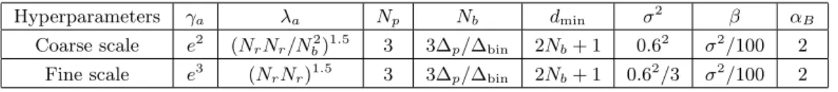
Table 2 Hyperparameter values.
Hyperparameters \gamma a \lambda a Np Nb d\mathrm{m}\mathrm{i}\mathrm{n} \sigma 2 \beta \alpha B
Coarse scale e2 (NrNr/Nb2)1.5 3 3\Delta p/\Delta \mathrm{b}\mathrm{i}\mathrm{n} 2Nb+ 1 0.62 \sigma 2/100 2
Fine scale e3 (NrNr)1.5 3 3\Delta p/\Delta \mathrm{b}\mathrm{i}\mathrm{n} 2Nb+ 1 0.62/3 \sigma 2/100 2
width and the pixel resolution.
\bullet The minimum distance between two points in the same pixel can be set as d\mathrm{m}\mathrm{i}\mathrm{n} =
2Nb+ 1, thus verifying the condition d\mathrm{m}\mathrm{i}\mathrm{n}> 2Nb.
\bullet The parameters controlling the number of points and the spatial correlation were set
by cross-validation using many Lidar datasets leading to \gamma a= e2 and \lambda a= (NrNc)1.5.
\bullet For each scale, we scaled the impulse response h\prime (t) = h(t) \=\lambda p
5\sum
th(t), where h(t) is
the unit gain impulse response, such that all intensity values lie approximately in
the interval [0, 10]. The regularization parameters were then fixed to \sigma 2 = 0.62 and
\beta = \sigma 2/100 by cross-validation in order to obtain smooth estimates.
\bullet The hyperparameter controlling the smoothness in the background image \bfitB was also
adjusted by cross-validation yielding \alpha B= 2.
Table 2summarizes the different hyperparameter values for the coarse and fine scales. All the
experiments were performed using Ni= 25NrNc iterations in the coarse scale and fine scale.
5.1. Error metrics. Three different error metrics are used to evaluate the performance of
the proposed algorithm. We compare the percentage of true detections F\mathrm{t}\mathrm{r}\mathrm{u}\mathrm{e}(\tau ) as a function
of the distance \tau , considering an estimated point as a true detection if there is another point
in the ground truth/reference point cloud in the same pixel (x\mathrm{t}\mathrm{r}\mathrm{u}\mathrm{e}
n = x\mathrm{e}\mathrm{s}\mathrm{t}n\prime and yn\mathrm{t}\mathrm{r}\mathrm{u}\mathrm{e} = yn\mathrm{e}\mathrm{s}\mathrm{t}\prime )
such that | t\mathrm{t}\mathrm{r}\mathrm{u}\mathrm{e}n - t\mathrm{e}\mathrm{s}\mathrm{t}
n\prime | \leq \tau . We also consider the number of points that were falsely created,
denoted as F\mathrm{f}\mathrm{a}\mathrm{l}\mathrm{s}\mathrm{e}(\tau ) (i.e., the estimated points that cannot be assigned to any true point at
a distance of \tau ). Regarding the intensity estimates, we focus on targetwise comparison, by gating the 3D reconstruction between the ranges where a specific target can be found, keeping only the point with biggest intensity and assigning zero intensity to the empty pixels. We compute the normalized mean squared error (NMSE) of the resulting 2D intensity image as
(5.1) NMSE\mathrm{t}\mathrm{a}\mathrm{r}\mathrm{g}\mathrm{e}\mathrm{t}=
\sum Nr
i=1
\sum Nr
j=1(r\mathrm{t}\mathrm{r}\mathrm{u}\mathrm{e}i,j - \^ri,j)2
\sum Nr i=1 \sum Nr j=1 \Bigl( r\mathrm{t}\mathrm{r}\mathrm{u}\mathrm{e} i,j \Bigr) 2 .
Finally, we consider the NMSE metric for the background image
(5.2) NMSE\bfitB =
\sum Nr
i=1
\sum Nr
j=1(b\mathrm{t}\mathrm{r}\mathrm{u}\mathrm{e}i,j - \^bi,j)2
\sum Nr i=1 \sum Nr j=1 \Bigl( b\mathrm{t}\mathrm{r}\mathrm{u}\mathrm{e} i,j \Bigr) 2 .
5.2. Synthetic data. We evaluated the algorithm in two synthetic datasets: a simple one, containing basic geometric shapes, and a complex one, based on a scene from the Middlebury
dataset [40]. Both scenes present multiple surfaces per pixel. The first scene, shown in
0
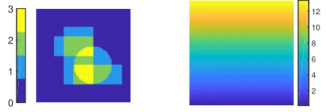
Figure 6. The 3D scene depicted inFigure 1consists of three plates with different sizes and orientations and one paraboloid-shaped object. Left: Number of objects per pixel. Right: Mean background photon count T \bfitB .
impulse response used in our experiments was obtained from real Lidar measurements, with attack = 58 bins and decay = 460 bins. The background was created using a linear intensity
profile, as shown in Figure 6. The resulting mean intensity per pixel was \=\lambda p = 11, meaning
that 99.75\% of the bins are empty and approximately 4 photons per pixel are due to 3D objects. First we evaluated the performance with and without the proposed priors to show their effect on the final estimates. The algorithm was tested in the following conditions:
1. with all the priors as reported in Table 2,
2. without spatial regularization (\gamma a= 1),
3. with a weak intensity regularization (\sigma 2= 1002),
4. with a softer spatial regularization for the background levels (\alpha B= 1),
5. without erosion and dilation moves,
6. only using the finest scale, adjusting the number of iterations to yield the same com-puting time.
The total execution time for all cases was approximately 120 seconds. Figure 7ashows F\mathrm{t}\mathrm{r}\mathrm{u}\mathrm{e}(\tau )
and F\mathrm{f}\mathrm{a}\mathrm{l}\mathrm{s}\mathrm{e}(\tau ) for all the configurations. The number of false points increases dramatically when
the area interaction process is not considered, as the sampler tends to create many points of low intensity, mistaking background counts as false surfaces. The background regularization does not affect the detected points significantly, but yields a better estimation of \bfitB , leading
to NMSE = 0.107 for \alpha B = 1 and NMSE = 0.0912 for \alpha B = 2. The number of true points
detected without dilation and erosion moves or using only one scale decreases dramatically to
44\% and 80\%, respectively. Figure 7b compares the estimated intensity of the biggest plate
with different values of \sigma 2. The NMSE obtained with \sigma 2 = 0.62 is 0.058, compared to 0.399
in the absence of correlation (i.e., when \sigma 2 = 1002). Section SM12 shows the performance of
ManiPoP for different SBRs and mean photons per pixel for this specific synthetic scene.
The second dataset was created with the ``Art"" scene from [40]. In order to have multiple
surfaces per pixel, we added a semitransparent plane in front of the scene. We simulated
the Lidar measurements, as if they were taken by the system described in [30]. The scene
consists of Nr = 183, Nc = 231 pixels, and T = 4500 histogram bins. The bin width is
\Delta b = 0.3 mm and the pixel size is \Delta p \approx 1.2 mm. In this complex scene, we compared
the proposed method with the optimization algorithms SPISTA and \ell 21+TV. SPISTA relies
on the specification of a background level that was set to the true background value. It is important to note that this information is not available in real Lidar applications, as the background levels depend on the imaged scene. We also show the results for the regularization
22 50 112 250
distance [mm]
100
102
104
False points found
22 50 112 250 distance [mm] 40 60 80 100
% of true points found
full weak spat. weak refl. 1 scale no dil. weak bgr.
(a) (b)
Figure 7. (a) shows the percentage of true (left) and false (right) detections. (b) shows the intensity estimates for the vertical plate: Ground truth (left), estimates with \sigma 2= 0.62 (center), and \sigma 2= 1002 (right).
parameter that attained best results among many trials (the empirical rule for setting this
parameter provided in [43] achieved worse results). We noticed that SPISTA provides large
errors in the intensity estimates, as the gradient of the Poisson likelihood is not Lipschitz
continuous and the gradient step iterations may diverge in very low photon scenarios [21,11].
This problem can be solved by using the SPIRAL [21] inner loop to compute the step size (see
section SM9 for details), yielding a new algorithm, which we name SPISTA+. The \ell 21+TV
algorithm has two regularization parameters that were adjusted in order to obtain the best results. It also relies on a thresholding step on the final estimates, as the output of the optimization method is not sparse. Again, the thresholding constant was adjusted to achieve
the best results. To further improve the results of \ell 21+TV, we included a grouping step,
similar to the one described in [43], which reduces the number of false detections by pairing
similar ones in the same pixel. Instead of taking the maximum intensity as in [43], we summed
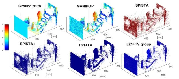
the intensities of the grouped detections, as this achieved better intensity estimates. Figure 8
shows the 3D point clouds obtained for each algorithm, whereas Figure 9shows F\mathrm{t}\mathrm{r}\mathrm{u}\mathrm{e}(\tau ) and
F\mathrm{f}\mathrm{a}\mathrm{l}\mathrm{s}\mathrm{e}(\tau ). SPISTA finds 18\% of the true points and around 5033 false detections, whereas
SPISTA+ improves the detection to 34\% and 4267 false detections. \ell 21+TV improves the
detection rate to 57\%, but also increases the false detections to 106. The grouping technique
improves the results provided by \ell 21+TV, reducing the false detections by a factor of 200. The
proposed method obtains the best results, finding 92\% of all the true points and 1852 false
detections. As shown in Table 3, the proposed algorithm yields the best intensity estimates
with the lowest execution time. Figure 10 shows the intensity estimate of the scene behind
the semitransparent plane for each algorithm. SPISTA fails to provide meaningful intensity results, whereas SPISTA+ yields better estimates. As all the points behind the plane are
grouped to yield a 2D intensity image, there is no difference between the \ell 21+TV and \ell 21+TV
with grouping. Both SPISTA+ and \ell 21+TV with grouping show a negative bias in the mean
intensity, which may be attributed to the effect of the \ell 1 and \ell 21 regularizations, respectively.
As both SPISTA+ and \ell 21+TV with grouping improve the results of the original algorithms
in all the evaluated datasets, we show only their results in the rest of the experiments.
5.3. Real Lidar data. We assessed the proposed algorithm using three different Lidar
datasets: the multilayered scene provided in [43,1] recorded at the Massachusetts Institute of
Technology, the polystyrene target imaged at Heriot-Watt University [5], and the camouflage
Figure 8. Estimated 3D point cloud by the proposed algorithm, SPISTA, SPISTA+, \ell 21+TV, and \ell 21+ T V with grouping. 1 3 8 distance [mm] 102 104 106
False points found
1 3 8
distance [mm]
0 50 100
% of true points found
MANIPOP SPISTA SPISTA+ L21+TV L21+TV group
Figure 9. Upper row: Percentage of true detections for different algorithms as a function of maximum distance \tau , Ftrue(\tau ). Bottom row: Number of false detections, Ftrue(\tau ).
Table 3
Performance of the proposed method, SPISTA, SPISTA+, \ell 21+TV, and \ell 21+TV with grouping on the
synthetic data.
Method Total time [seconds] NMSE intensity
SPISTA [43] 712 > 1
SPISTA+ 8161 0.993
\ell 21+TV [19] 2453 0.845
\ell 21+TV group 2455 0.845
ManiPoP \bfsix \bfthree \bfzero \bfzero .\bfzero \bfnine \bfnine \bfnine
4000 3500 MANIPOP 3000 [mm] 2500 2000 1500 4000 3500 SPISTA+ 3000 [mm] 2500 2000 1500 4000 3500 L21+TV group 3000 [mm] 2500 2000 1500 0 10 20 30
Figure 11. Estimated 3D point cloud by ManiPoP, SPISTA, \ell 21+TV, and \ell 21+TV with grouping.
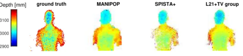
MANIPOP SPISTA+ L21+TV group
2900 3000 3100
ground truth
Depth [mm]
Figure 12. Depth estimates of the mannequin. From left to right: Long acquisition reference, ManiPoP, SPISTA+, and \ell 21+TV with grouping estimates.
5.3.1. Mannequin behind a scattering object. The first scene consists of a mannequin
located 4 meters behind a partially scattering object, with Nr= Nc= 100 pixels and T = 4000
bins. This Lidar scene is publicly available online [1]. The mean photon count per pixel is
\=
\lambda p= 45, and the dimensions are \Delta p \approx 8.4 mm and \Delta b = 1.2 mm. In [43], a Gaussian-shaped
impulse response is suggested. However, we used a data-driven impulse response that yields
better results (seesection SM10for a detailed explanation). Figure 11shows the reconstructed
point clouds for each algorithm. ManiPoP achieves a sparse and smooth solution, whereas the
estimate of SPISTA presents more random scattering of points. The \ell 21+TV output presents
more spatial structure than SPISTA, but also fails to find the border of the mannequin. The dataset contains a reference depth of the mannequin obtained using a long acquisition time. This reference was computed using the log-matched filtering solution of a cropped Lidar
cuboid where only the mannequin is present. Figure 12shows the ground truth depth and the
estimates obtained by ManiPoP, SPISTA+, and \ell 21+TV with grouping. The proposed method
outperforms the SPISTA+ and \ell 21+TV outputs, finding 97.9\% of the reference detections,
whereas SPISTA+ only detects 74.8\% and \ell 21+TV with grouping finds 92.8\%, as shown in
Figure 13. The SPISTA+ and \ell 21+TV with grouping algorithms detect 225 and 206 false
points, respectively, compared to the 432 points found by ManiPoP. This increase in false detections can be attributed to the scattering object that was (probably) removed when the
reference dataset was obtained. The scattering effect can be also seen in Figure 11, as it is
possible to find some parts of the low intensity surface behind the mannequin. Despite not having a reference for reflectivity values of the target, we can say that the proposed method
attains significantly better visual results, as shown inFigure 14. Both SPISTA+ and \ell 21+TV
with grouping underestimate the mean intensity. The total execution time of ManiPoP (146 seconds) was around 20 times less than SPISTA+ (2871 seconds) and slightly shorter than
Figure 13.Percentage of true detections at a maximum distance \tau , Ftrue(\tau ), for ManiPoP, SPISTA+, and
\ell 21+TV with grouping. The number of false detections, Ffalse(\tau ), is shown in (b).
MANIPOP SPISTA+ L21+TV group
0 10 20 30
Figure 14. Estimated intensity by ManiPoP, SPISTA+, and \ell 21+TV with grouping. The colorbar
illus-trates the number of photons assigned to each point. Both SPISTA+ and \ell 21+TV show a negative bias in the
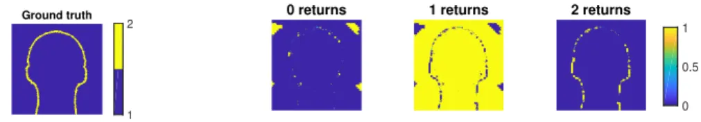
mean intensity. Ground truth 1 2 0 returns 0 0.5 1 1 returns 2 returns
Figure 15.From left to right: True number of surfaces per pixel and probability of having k = 0, 1, 2 objects per pixel for an acquisition time of 1 ms, respectively.
5.3.2. Polystyrene head. The second dataset was obtained in Heriot-Watt University and consists of a life-sized polystyrene head at 40 meters from the imaging device (an image can
be found in [5]). The data cuboid has size Nr = Nc = 141 pixels and T = 4613 bins. The
physical dimensions are \Delta p \approx 2.1 mm and \Delta \mathrm{b}\mathrm{i}\mathrm{n} = 0.3 mm. A total acquisition time of 100
milliseconds was used for each pixel, yielding \lambda p = 337 with approximately 23 background
photons per pixel. The scene consists mainly of one object per pixel, only with two surfaces per pixel around the borders of the head. We compare the proposed method with the log-matched filtering solution and the SPISTA+ algorithm for different acquisition times, i.e.,
many values of \lambda p. As no ground truth is available, we used as reference the log-matched
filter solution, manually dividing the Lidar cube into segments with only one surface, using the largest acquisition time (100 ms). Although the dataset seems to have only one active depth per pixel, two surfaces per pixel can be found in the borders of the head, as shown in Figure 15. As only a few pixels contain two surfaces, we also compared with [38], which is a state-of-the-art 3D reconstruction algorithm under a single-surface-per-pixel assumption.
Figure 16 shows the reconstructed 3D point clouds for an acquisition time of 1 ms, whereas
Figure 17 shows F\mathrm{t}\mathrm{r}\mathrm{u}\mathrm{e}(\tau ) and F\mathrm{f}\mathrm{a}\mathrm{l}\mathrm{s}\mathrm{e}(\tau ) for acquisition times of 10, 1, and 0.2 ms. In the 10
800 MANIPOP [mm] 600 400 0 2 4 6 800 Log-matched filter [mm] 600 400 800 SPISTA+ [mm] 600 400 800 L21+TV group [mm] 600 400 800
Rapp and Goyal 2017
[mm]
600 400
Figure 16. Estimated 3D point clouds using the polystyrene head dataset with an acquisition time of 1 ms. SPISTA+ and \ell 21+TV underestimate the mean intensity, whereas ManiPoP, the log-matched filter solution,
and [38] obtain a similar intensity mean.
1 4 13 48
distance [mm]
102 104
False points found
1 4 13 48
distance [mm]
0 50 100
% of true points found
MANIPOP Log-matched filter SPISTA+ L21+TV group Superpixel Unmixing
0 50 100 102 104 0 50 100 105
Figure 17. Ftrue(\tau ) and Ffalse(\tau ) for the polystyrene head using acquisition times of 10 ms (top), 1 ms
(middle), and 0.2 ms (bottom). While all methods obtain good reconstructions in the 10 ms case, ManiPoP and [38] also achieve good reconstructions with acquisition times of 1 ms and 0.2 ms.
providing relatively few false estimates. The log-matched filter solution (of the complete Lidar cube) shows a significant error in depth estimates and fails to find 10\% of true points, as it
is only capable of finding one object per pixel. In the 0.2 ms case, there are only \lambda p = 0.7
photons per pixel on average. Thus, the best performing algorithm is [38], as the single-surface
assumption plays a fundamental role in inpainting the missing depth information. ManiPoP
performs in second place, finding 14\% fewer true points than [38].
As shown in Table4, the fastest algorithm is the log-matched filtering solution with less
than 20 seconds in all cases. However, ManiPoP still requires less computing time than
SPISTA+ and \ell 21+TV with grouping. It is worth noticing that the \ell 21+TV algorithm has a
memory requirement proportional to 6 times the whole data cube due to the ADMM algorithm, which can be prohibitively large when the Lidar cube is relatively big. The sparse nature of the ManiPoP algorithm only requires an amount of memory proportional to the number of bins with one photon or more plus the number of 3D points to infer.
To further demonstrate the generality of the proposed method, we studied the case where only one surface is present per pixel, but not all the pixels contain surfaces, which occurs in