Efficient algorithm for general polygon clipping

HAL Id: inria-00517687

https://hal.inria.fr/inria-00517687

Submitted on 15 Sep 2010

HAL is a multi-disciplinary open access archive for the deposit and dissemination of sci-entific research documents, whether they are pub-lished or not. The documents may come from teaching and research institutions in France or abroad, or from public or private research centers.

L’archive ouverte pluridisciplinaire HAL, est destinée au dépôt et à la diffusion de documents scientifiques de niveau recherche, publiés ou non, émanant des établissements d’enseignement et de recherche français ou étrangers, des laboratoires publics ou privés.

Efficient algorithm for general polygon clipping

Yu Peng, Junhai Yong, Hui Zhang, Jiaguang Sun

To cite this version:

Yu Peng, Junhai Yong, Hui Zhang, Jiaguang Sun. Efficient algorithm for general polygon clipping. Proceedings of The 6th International Conference on Computer-Aided Industrial Design and Concep-tual Design 2005, May 2005, Delft, Netherlands. �inria-00517687�

EFFICIENT ALGORITHM FOR GENERAL POLYGON CLIPPING

Yu Peng

1,2

Junhai Yong

1

Hui Zhang

1

Jiaguang Sun

1,2 1_{School of Software, Tsinghua University, Email:}

pengyu00@mails.tsinghua.edu.cn 2_{Department of Computer Science and Technology, Tsinghua University}

ABSTRACT: We present an efficient algorithm to determine

the intersection of two planar general polygons. A new method based on rotation angle is proposed to obtain the classification of an edge with respect to a polygon. The edge candidates can be determined efficiently by a 1-dimensional range searching approach based on an AVL tree (a balanced binary search tree). The simplicial chain is used to represent the general polygons, and to determine the classification of polygon edges. Examples are given to illustrate the algorithm.

KEYWORDS: Computational geometry, Geometric

modeling, Polygon intersection, Polygon Clipping, AVL tree.

1. INTRODUCTION

Polygon clipping with applications in various areas of computer graphics [7, 15] and CAD (Computer Aided Design) [4, 9] is one of the fundamental problems of the computational geometry

[1, 10, 12]. In literature lots of approaches for polygon clipping are presented [5, 6, 8, 11, 13-16]. Peng et al

[8] have made a good summarization of the latest research directions on this problem, and proposed a simpler, more efficient and more robust algorithm to determine the intersection of two general polygons with respect to the algorithm by Rivero and Feito [11]. The algorithm uses a process of double-nested loop to determine all edges of a polygon that are contained within the simplices of other polygon, which would spend time on some useless calculation.

A more efficient algorithm is presented in this paper. As with the algorithm by Peng et al [8], we adopt the simplex theory to handle general polygons. In Peng et al algorithm, each inclusion test between an edge midpoint of one polygon and a simplex of the other is performed. Practically, however, an edge midpoint of one polygon is contained within no or only a few simplices of the other. In the new algorithm, the process of double-nested loop is reduced to a 1D range searching using an AVL tree. The new algorithm is more efficient, as it requires half as much running time as the algorithm presented by Peng et al does.

2. PRELIMINARIES

We begin by briefly reviewing some definitions

and properties about simplicial chain by Feito et al [3] and Peng el al [8]. (Refer to [2, 3, 8] for more details).

A general planar polygon is a single polygon or a polygon consisting of a set of non-intersecting single polygons. The boundary of a single polygon consists of an outer contour and several non-intersecting inner contours. Each contour is represented by several directed edges and may be convex or concave. The outer contour is oriented in counterclockwise and the inner contours in clockwise. Thus, the interior of the polygon is on the left side of each directed edges.

A simplex S is an ordered triangle, and the coefficient of S equals sign(Area_sign(S)), where sign is the sign function and Area_sign is the signed area of the ordered triangle. In the remaining part of this paper, the simplex is referred to an original simplex, where a vertex of the simplex lies on the origin. The directed edge, an endpoint of which lies on the origin, is called an original edge (otherwise called a non-original edge). A simplicial chain is a collection of the sequence of the simplices {Si} and the sequence

of the coefficients {αi}, and it is denoted by λ=∑αi·Si,

where i=1, 2, ..., n.

Definition 1. Given a simplicial chain λ=∑αi·Si, for

any point Q

∈

R2, a characteristic function fλ is defined

by ⎪⎩ ⎪ ⎨ ⎧ =

_∑

= n i i i -f 1 otherwise. , of edge original non on the is , 1 ) ( _β λ S Q Q (1) where ⎪ ⎪ ⎩ ⎪⎪ ⎨ ⎧ = . S S otherwise , of edge original some on is if , of region open the inside is if , 0 , 2 1 , i i i i i a a Q Q β (2)

The closed set of the point set given by Pλ={Q |

fλ(Q)=1, Q

∈

R2} is a polygon, and λ is called the

simplicial chain associated with the polygon. Given a general polygon, we could find its associated simplicial chain.

e1, e2,..., en. Let Si be the original simplex determined

by the origin and ei, and let αi be the coefficient of Si,

where i=1, 2, ..., n. Then λ=∑αi·Si is the simplicial

chain associated with polygon P.

O e1 e2 e3 S3 (a) O (d) S1 (b) S2 O _(c) O 0 ) (Q= λ f fλ(Q)=1 fλ(Q)=-1 2 1S S− − = λ 1 S − = λ λ=−S1−S2+S3

Figure 1. associated simplicial chain of given triangle

Figure 1 gives an example of an associated simplicial chain of a triangle. This paper assumes that the general polygons are in the first quadrant. A translation is enough to move any general polygons into the first quadrant if it is necessary to do so. Given two general polygons, the subdivision process is as follows. First, calculate intersection points and touching points (some edges’ endpoints lying on other edges) of two general polygons. Then subdivide the directed edges of two polygons into smaller directed edges at the intersection points and the touching points. Finally, establish the new general polygons from the subdivided directed edges.

Theorem 1. Let P1 and P2 be two general polygons

after the subdivision process, and ev be a directed edge of P1. Assume that neither nor -ev ev is a directed edge of P2. Then, ev is inside P2 if and only if the midpoint of ev is in P2.

Definition 2. Let P1 and P2 be two given general

polygons after the subdivision process. Let λ be the simplicial chain of P2. For any directed edge ev of P1, the characteristic function f of ev on P2 is given by

⎪ ⎩ ⎪ ⎨ ⎧ = otherwise. , of edge directed a is - if , of edge directed a is if ), ( , 0 , 1 ) ( ₂ 2 P P Q e e f e f v v v λ (3)

where Q is the midpoint of e , and fλ(Q) is

defined by Eqn. (1).

v

Corollary 1. Let ev be a directed edge of P1. Then,

ev is contained within P2 if and only if f( ev )=1, where

f( e ) is defined by Eqn. (3). v

The following theorem uses the simplex theory to obtain the clipped polygon of two given polygons.

Theorem 2. Given two general polygons P1 and P2

after the subdivision process. Then, the associated simplicial chain of the clipped polygon P3=P1∩P2 is

∑

∑

∑

⋅ + ′⋅ ′ + ⋅ = ai Si aj Sj bk Uk 3 P λ (4) where i =1, 2, ..., n, j=1, 2, ..., n', k=1, 2, ..., l, {Si}

and {S'j} are two subsets consisting of the simplices of P1, respectively. The non-original edge of each Si is

inside P2, and the non-original edge of each S'j is

equivalent to some directed edge of P2. {Uk} is a

subset consisting of the simplices of P2. The non-original edge of each Uk is inside P1. {ai}, {a'j}

and {bk} are the coefficient sets of simplices of {Si},

{S'j} and {Uk}, respectively.

3. ROTATION ANGLE

In order to obtain an efficient algorithm, we need some new definitions and terminology.

Definition 3. Given a point, the rotation angle of the

point is given by the counterclockwise angle that the positive x-axis makes with the segment from the origin to the point.

As shown in Figure 2, α, β and γ are the rotation angles of the points p1 , p2 and p3, respectively. From the feature of the rotation angle of a point, we could have the following theorem.

S O y x p2 1 θ θ2 α p1 p3 β γ A B

Figure 2. Rotation angle of points

Theorem 3. Given an original simplex and a point in

the first quadrant. The point is inside the simplex, if and only if the following two conditions are both satisfied:

z The rotation angle of the point is in the range [x:x']. z Both the origin and the point are on the same side of the non-original edge of the original simplex.

Where x and x' are the rotation angles of two endpoints of the non-original edge of the original simplex, respectively.

As shown in Figure 2, p2 is inside the simplex S. The rotation angle β of p2 is in the range [θ1:θ2], and both the origin and p2 are on the same side of the edge

AB, where θ1 and θ2 are the rotation angles of B and

A, respectively. The situation of neither p1 nor p3

satisfies the above two conditions simultaneously, where the rotation angle of p1 is greater than θ1, and the origin and p3 are not on the same side of AB).

Hence, neither p1 nor p3 is inside S.

Definition 4. Given a general polygon and an original

simplex in the first quadrant, an edge of the polygon is called an edge candidate with respect to the simplex if and only if the rotation angle of the edge midpoint is in the range [x:x'], where x and x' are the rotation angles of two endpoints of the non-original edge of the original simplex, respectively.

4. CLIPPING ALGORITHM

The new algorithm is based on the simplex theory mentioned in Section 2. The pseudo code for the algorithm is illustrated in Figure 3.

Algorithm CLIPPING (P1,P2,P3) Input. two general polygon P1 and P2. Output. the clipped polygon P3= P1∩P2.

/* P1* and P2* are the polygons after subdivision. */

1. SUBDIVISIONPROCESS (P1,P2,P1*,P2*);

/* λ1* is the associated simplicial chain of P1*. */

2. BUILDSIMPLICIALCHAIN (P1*,λ1*);

/* λ2* is the associated simplicial chain of P2*. */

3. BUILDSIMPLICIALCHAIN (P2*,λ2*);

/* si* _{is the non-original edges of the simplices Si}* _{from λ}

1*; f(si*) is the

characteristic function of si* _{on P}

2 according to Definition 2; SUBJECT

means that P1* is the subject polygon.*/

4. CALEDGECHARACTER (P1*,P2,λ1*,λ2,f(si*),SUBJECT);

/* uj* _{is the non-original edges of the simplices Uj}* _{from λ}

2*; f(uj*) is the

characteristic function of uj* _{on P}

1; CLIP means that P2* is the clip

polygon.*/

5. CALEDGECHARACTER (P2*,P1,λ2*,λ1,f(uj*),CLIP);

/* Calculate the resultant simplicial chain λ3 through λ1* and λ2* using

Theorem 2. */

6. CALRESULTCHAIN (λ1*,f(si*),λ3); 7. CALRESULTCHAIN (λ2*,f(uj*),λ3);

Figure 3. Pseudo code for clipping algorithm

At first, the subdivision process is performed on the given general polygons. Then, build the simplicial chains for both polygons according to Lemma 1, and calculate the value of the characteristic function for each edge of one polygon on the other’s original polygon (the polygon before the subdivision process) through Corollary 1. At last, the simplicial chain of the clipped polygon P3 is obtained through a subroutine CALRESULTCHAIN shown in Figure 4, and we have the polygon P3 from the simplicial chain.

CALRESULTCHAIN (λ,f(si),λ3)

Input. The simplicial chain λ and the characteristic function f(si) Output. The resultant simplicial chain λ3.

1. for each simplex Si of λ do

2. if f(si)=1 then /* si is the non-original edge of Si. */

3. Add the simplex Si and its coefficient to λ3;

Figure 4. Pseudo code for calculating the resultant

simplicial chain

The subdivision process is already described in Section 2. How to build a simplicial chain of a general polygon is introduced in Lemma 1. According to Definition 2 and Corollary 1, we could obtain the value of an edge characteristic function of a polygon by calculating the classification between the edge midpoint and each simplex of the other. Practically, however, an edge midpoint of one polygon is contained within no or only a few simplices of the other.

In order to accelerate the calculation of value of the edge characteristic function, we extend the 1-dimensional range searching approach [1] with the

principles described in Section 3. The edge candidates can be determined by this approach efficiently. The pseudo code for calculating values of edge characteristic functions is illustrated in Figure 5.

CALEDGECHARACTER (P1,P2,λ1,λ2,f(si),t)

Input. Two polygons P1 and P2 and their respective simplicial

chains λ1 and λ2, t denotes the type of P1.

Output. The characteristic function f(si) of si on P2.

/* Initiate the function f(si); si is the non-original edge of Si.*/ 1. for each simplex Si of λ1 do

2. f(si)←0;

/* Build the 1D range searching tree; T is the AVL tree */ 3. BUILD1DRANGETREE (λ1,f(si),P2,T,t); 4. for each simplex Uj of λ2 do

/* uj is the non-original edge of Uj. */

5. x ← the minor rotation angle of endpoints of uj;

6. x' ← the major rotation angle of endpoints of uj;

/* vs is the split node; [x:x'] is the 1D query range with x ≤ x'. */

7. vs ← FINDSPLITNODE (T,[x:x']); 8. if vs≠ NULL then

/* ra(vs) denotes the rotation angle stored at vs. */

9. if ra(vs) is in [x:x'] then

/* Calculate f(s(vs)); s(vs) denotes the directed edge stored at vs. */

10. CALVAL (f(s(vs)),Uj);

11. if vs is not a leaf then

/* Follow the path to x and calculate the characteristic functions of the edge candidates; lc(vs) denotes the left child of vs. */

12. v ← lc(vs); 13. while v ≠ NULL do 14. if ra(v) ≥ x then 15. CALVAL (f(s(v)),Uj);

/* Traverse the subtree rooted at rc(v); rc(v) denotes the right child of v. */ 16. CALSUBTREEVAL (rc(v),f(s(rc(v))),Uj);

17. v ← lc(v); 18. else v ← rc(v);

19. Follow the path to x'_{, calculate the characteristic}

functions of the edge candidates, which is similar to lines 12-18.

Figure 5. Pseudo code for calculating the values of

edge the characteristic functions

Now we describe CALEDGECHARACTER in more details. First initiate the edge characteristic functions in line 1 and line 2. Then build the AVL tree T in line 3. Each node of T stores a directed edge of one polygon and the rotation angle of the edge midpoint. We assume that the left subtree of a node v contains all the rotation angles smaller than or equal to ra(v) and that the right subtree contains all the rotation angles strictly greater than ra(v). In lines 4-19, we traverse each simplex of the other polygon. For each simplex, we adopt the 1-dimensional range searching approach to determine the nodes, where the rotation angles stored at the nodes are in the range [x:x']. To find these nodes we first search for the node vs in line 7, where the paths to x and x' _{split shown in Figure 6.}

FINDSPLITNODE (T,[x:x'_])

Input. An AVL tree T and the query range [x:x'] with x ≤ x'. Output. The node v where the paths to x and x' split.

1. v ← the root of T;

child and right child of v, respectively. */

2. while v ≠ NULL and (ra(v) < x or ra(v) ≥ x') do

3. if (ra(v) ≥ x') then 4. v ← lc(v); 5. else v ← rc(v); 6. return v;

Figure 6. Pseudo code for finding the split node

Starting from vs we then follow search path of x. At each node where the path goes left, we first calculate the characteristic function of the edge stored at it through a subroutine CALVAL, and then do the same calculation on each node in the right subtree, since this subtree is between the two search paths, i.e., the edges stored at the nodes in the subtree are the edge candidates. CALSUBTREEVAL is recursive and it is used to calculate the characteristic functions of all nodes in the subtree (The subroutine is illustrated in

Figure 7). Similarly, follow the path of x' and calculate the characteristic functions of the edge candidates.

CALSUBTREEVAL (v,f(s),U)

Input. A node v in the AVL tree and a simplex U. Output. The edge characteristic function f(s).

/* s(v) denotes the directed edge stored at v; lc(v) denotes the left child of v; rc(v) denotes the right child of v.*/

1. if v ≠ NULL then 2. CALVAL (f(s(v)),U);

3. CALSUBTREEVAL (lc(v),f(s(lc(v))),U);

4. CALSUBTREEVAL (rc(v),f(s(rc(v))),U);

Figure 7. Pseudo code for calculating the values of

the edges stored at the subtree

The pseudo code for building AVL tree is shown in Figure 8. According to Definition 2, when a directed edge is shared by two polygons both values of the characteristic functions of this edge on respective polygons are 1. And according to Eqn. (4), only one corresponding simplex of this edge is added to the resultant simplicial chain. Hence, we force

f(si)=1 in line 6 of BUILD1DRANGETREE, where si is

from the subject polygon and it is shared by both polygons.

BUILD1DRANGETREE (λ,f(si),P2,T,t)

Input. The simplicial chains λ and the type t of the polygon

associated with λ.

Output. An AVL tree T and the characteristic function f(si) on

polygon P2.

1. for each simplex Si of λ do

/* si is the non-original edge of Si; */

2. if si does not overlap any edges of P2 then 3. p ← the rotation angle of the midpoint of si;

4. Insert node (si,p) into T;

/* It is performed according to Definition 2; */

5. else if t = SUBJECT and si is a directed edge of P2 then 6. f(si) ← 1;

Figure 8. Pseudo code for building 1D range tree

The subroutine CALVAL is illustrated in Figure 9. It uses Theorem 3 to determine the classification of

the edge midpoint in line 1, and the characteristic function of the edge s is calculated in line 3 and line 4 according to Definition 1 and Definition 2.

CALVAL (f(s), U)

Input. A directed edge s and a simplex U. Output. The edge characteristic function f(s).

/* Obtain the classification by Theorem 3; u is the non-original edge of U. */ 1. if Both the midpoint of s and the origin are on the same

side of u then

/* a(s) denotes the rotation angle of the midpoint of s; mina(u) denotes the minor rotation angle of vertices of u; maxa(u) denotes the major rotation angle of vertices of u; c(U) denotes the coefficient of U. */

2. if a(s) = mina(u) or a(s) = maxa(u) then 3. f(s) ← f(s)+ c(U)/2;

4. else f(s) ← f(s)+c(U);

Figure 9. Pseudo code for calculating the value of an

edge to a simplex

5.

EVALUTION

5.1 Time Complexity

Let n and m be the numbers of edges of the two polygons P1 and P2, respectively, and k be the number of the intersection points and the touching points of P1 and P2. For the subdivision process, we adopt the plane sweep algorithm introduced in References [1, 10, 12] to calculate the intersection points and touching points. Therefore, the running time required by the subdivision process is O((n+m)log(n+m)+k). The subroutine BUILDSIMPLICIALCHAIN takes an amount of time that is linear in the number of edges of the polygon. CALEDGECHARACTER with respect to the subject polygon uses a loop, which includes the 1D range searching process. The AVL tree can be built in

O((n+k)log(n+k)) time. FINDSPLITNODE takes

O(log(n+k)) time. The time spent in a call to

CALSUBTREEVAL is linear in ti, where ti is the number

of the edge canditates of subject polygon with respect to the ith simplex of clip polygon. Hence, the total time spent in such call s is O(ti). The remaining nodes

storing the edge candidates are the nodes on the search path of x or x'. Because T is balanced, these paths have length O(log(n+k)), so the total time spent in these nodes is O(log(n+k)). Hence, the time of 1D range searching process is O((log(n+k))+ti). Since the

1D range searching process runs m times in the loop, the subroutine CALEDGECHARACTER with respect to subject polygon gives a running time of

O(mlog(n+k)+T1)), where T1=∑ti. Similarly,

CALEDGECHARACTER with respect to clip polygon gives a running time of O(nlog(m+k)+T2), where

T2=∑sj and sj is the number of the edge canditates of

clip polygon with respect to the jth simplex of subject polygon. The subroutine CALRESULTCHAIN gives a time of O(n+m+k).

5.2 Example

Next we show an example in which two polygons have some edges in common. Figure 10(a) shows the subject polygons P1 and the clip polygon P2.

S1 S2 O x y (a) U1 S1* S5* S4* S3* S2* S7* S6* O x y (b) S8* S4 S5 S6 S3 U2 U3 U4 U5 U6 U1* S11* S12* U8* U9* U5* U4* U3* U7* U2* U6* S10* S9* P1 P2 P1* P2*

Figure 10. Example: (a) two polygons with their

associated simplicial chains, (b) the clipped polygon (in deep gray)

The simplical chains of P1 and P2 are

λ1=S1-S2+S3-S4+S5-S6 and λ2=-U1-U2+U3-U4-U5+U6, respectively. The new algorithm first performs the subdivision process on the two general polygons according to not only the intersection points but also the touching points. After the subdivision process, the simplical chains of P1* and P2* are λ1* = S1* - S2* - S3* -

S4*+S5*+S6*+S7*-S8*-S9*+S10*+S11*-S12* and λ2* = -U1* -U2*-U3*-U4*-U5*+U6*-U7*-U8*+U9*, respectively. The simplex S3* is equivalent to the simplex U5*, and the non-orginal edge of S5* has the opposite orientation as the non-original edge of U7*.

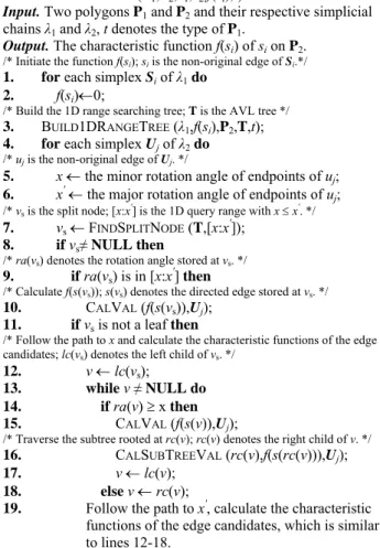
Table 1 shows the procedure for calculating the values of the edge characteristic functions of P1* on P2. The simplices of P1* and P2 and their coefficients are shown in the first row and the first column of Table 1, respectively. The second row lists the query range of each simplex of P2. The second column lists the rotation angle of the midpoint of each edge of P1*. Note that the value of the charactristic functions of the edges, which overlap some edges of P2*, can be determined directly through the edge directions. Hence, fill the corresponding bracket with ‘+’ where the corresponding Si* and Uj have the non-original

edges in common that have the same orientation, and fill the bracket with ‘−’ where the corresponding Si*

and Uj have the non-original edges in common that

have the opposite orientations. Assume that the midpoint of the non-original edge of Si* and the

simplex Uj are the point and the simplex in the

assumed conditions of Theorem 3, respectively. In the interior of Table 1, the corresponding table cell leaves with blank where the first condition of Theorem 3 is not satisfied. The cell is filled with ‘°’ where only the first condition of Theorem 3 is satisfied. The cell is filled with ‘3’ where both of the two conditions of Theorem 3 are satisfied. The last column lists the value of the characteristic function of non-original edge of respective Si* according to Definition 2.

Table 1. Procedure for calculating the value of edge

characteristic functions of P1* P2→ U1(-1) U2(-1) U3(1) U4(-1) U5(-1) U6(1) f(si*) range→ P1*↓ _angle↓ [33.7:38.7] [26.6:33.7] [26.6:29.1] [21.8:29.1] [15.9:21.8] [15.9:38.7] S1*(1) (56.3) 0 S2*(-1) (45.0) 0 S3*(-1) (+) 1 S4*(-1) (24.0) 3 3 -1+1=0 S5*(1) (−) 0 S6*(1) (32.9) ° 3 1 S7*(1) (45.0) 0 S8*(-1) (42.1) 0 S9*(-1) (33.2) ° 3 1 S10*(1) (32.6) ° 3 1 S11*(1) (41.3) 0 S12*(-1) (48.7) 0

Similarly, Table 2 shows the procedure for calculating the values of the edge characteristic functions of P2* on P1. The value of last column of

Table 2 is zero where the corresponding bracket of the second column is filled with ‘+’ or ‘−’. The simplices, whose corresponding numbers in the last columns of

Table 1 and Table 2 are 1, are selected to build the resultant simplicial chain of clipped polygon. Hence, the resultant simplicial chain is λ3 = S3*+ S6*- S9*+

S10*- U2*-U4*+U6*. The clipped polygon is indicated in deep gray shown in Figure 10(b).

Table 2. Procedure for calculating the value of edge

characteristic functions of P2*

5.3 Experimental results

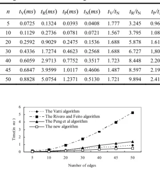
Performance data of the Vatti algorithm, the Rivero and Feito algorithm, the Peng et al algorithm and the new algorithm are shown in Table 3 and

Figure 11. All algorithms were implemented in a personal computer with 1.7GHZ Intel Pentium IV CPU and 256MB RAM, and the source code of all four algorithms are complied with the Microsoft Visual C++ 6.0 compiler using the same byte alignment (8 bytes) and optimization options. In Table 3, the numbers of edges in both general polygons are listed in the first column, i.e., both general polygons have the same number of edges. The numbers below

tV, tR, tP and tN are the running times (in milliseconds) respectively used to calculate the intersection results for the Vatti algorithm, the Rivero and Feito algorithm,

P1→ S1(1) S2(-1) S3(1) S4(-1) S5(1) S6(-1) f(uj*) range→ P2*↓ angle↓ [53.1:63.4] [21.8:63.4] [21.8:53.1] [30.4:48.2] [30.4:49.6] [48.2:49.6] U1*(-1) (37.9) ° ° ° ° 0 U2*(-1) (36.5) ° 3 ° ° 1 U3*(-1) (35.6) ° 3 3 ° 1-1=0 U4*(-1) (34.4) ° 3 3 3 1-1+1=1 U5*(-1) (+) 0 U6*(1) (27.9) ° 3 1 U7*(-1) (−) 0 U8*(-1) (18.4) 0 U9*(1) (26.6) ° ° 0

the Peng et al algorithm and the new algorithm. We used a very large number of examples to test the four algorithms. The running time was obtained by averaging. The improvement factors of the new algorithm over other algorithms are also listed in

Table 3 (from the 6th column to the 8th column). In

Figure 11 we can see graphically the evolution of the running time of polygon clipping versus the number of polygon edges used for our algorithm and the other algorithms. As we can see in the results, the new algorithm is more efficient. The running time required by the new algorithm is less than one third of that by the Rivero and Feito algorithm and half as much as that by the Peng et al algorithm.

Table 3. Performance results using: the Vatti

algorithm, the Rivero and Feito algorithm, the Peng et al algorithm and the new algorithm

n tV(ms) tR(ms) tP(ms) tN(ms) tV/tN tR/tN tP/tN 5 0.0725 0.1324 0.0393 0.0408 1.777 3.245 0.963 10 0.1129 0.2736 0.0781 0.0721 1.567 3.795 1.083 20 0.2592 0.9029 0.2475 0.1536 1.688 5.878 1.611 30 0.4336 1.7274 0.4623 0.2568 1.688 6.727 1,800 40 0.6059 2.9713 0.7752 0.3517 1.723 8.448 2.204 45 0.6847 3.9599 1.0117 0.4606 1.487 8.597 2.196 50 0.8828 5.0754 1.2371 0.5130 1.721 9.894 2.412 0 1 2 3 4 5 6 5 10 20 30 40 45 50 Number of edges Ti me (i n ms )

The Vatti algorithm The Rivero and Feito algorithm The Peng et al algorithm The new algorithm

Figure 11. Performance chart using: the Vatti

algorithm, the Rivero and Feito algorithm, the Peng et al algorithm and the new algorithm

6. CONCLUSIONS

In this paper, a new polygon clipping algorithm is presented. A new method based on the rotation angle of the edge midpoint is used to determine the classification of the edges of a polygon with respect to another polygon. Also the edge candidate is defined by the rotation angle and a 1-dimensional range searching approach is proposed to obtain the edge candidates for accelerating the edge classification. The algorithm is efficient, as it requires half as much running time as the algorithm by Peng et aldoes.

ACKNOWLEDGMENTS

The research was supported by the National Science Foundation of China (60403047) and the Chinese 973 Program (2004CB719400). The second author was supported by a Foundation for the Author of National Excellent Doctoral Dissertation of PR China (200342) and a project sponsored by SRF for ROCS, SEM.

REFERENCE

[1] de Berg, M., van Krefeld, M., Overmars, M., Schwarzkopf, O., Computational Geometry: Algorithms and Applications, Springer-Verlag, 1997.

[2] Feito, F.R., Torres, J.C., Ureña, A., Orientation, simplicity and inclusion test for planar polygons, Computers & Graphics 1995; 19(14): 595-600.

[3] Feito, F.R., Rivero, M.L., Geometric Modelling based on simplicial chains, Computers & Graphics 1998; 22(5): 611-619.

[4] Hoffmann, C.M., Hopcroft, J.E., Karasick, M.J., Robust set operations on polyhedral solids, IEEE Computer Graphics and Applications, Vol. 9, No. 6, 1989, pp 50-59. [5] Greiner, G., Hormann, K., Efficient clipping of arbitrary

polygons, ACM Transactions on Graphics 1998; 17(2): 71-83.

[6] Liang, Y.-D., Barsky, B.A., An analysis and algorithm for polygon clipping, Communications of the ACM 1983; 26(11): 868-877.

[7] Loutrel, P.P., A solution to the hidden-line problem for computer-drawn polyhedra, IEEE Transactions on Computers 1970; 19(3): 205-213.

[8] Peng, Y., Yong, J.-H., Sun, J.-G., A new algorithm for Boolean operation on general polygons, Computers & Graphics 2005; 29(1): to appear.

[9] Persion, H., NC machining of arbitrarily shaped pockets, Computer-Aided Design 1978; 10(3): 169-174.

[10] Preparata, F.P., Shamos, M.I., Computational geometry: an introduction, Berlin: Springer-Verlag, 1985.

[11] Rivero, M.L., Feito, F.R., Boolean operations on general planar polygons, Computers & Graphics 2000; 24(6): 881-896.

[12] O’Rourke, J., Computational geometry in C, Cambridge: Cambridge University Press, 1985.

[13] Schutte, K., An edge labeling approach to concave polygon clipping, Manuscript, 1995; 1-10.

[14] Sutherland, I.E., Hodgeman, G.W., Reentrant polygon clipping, Communications of the ACM 1974; 17(1): 32-42.

[15] Weiler, K., Atherton, P., Hidden surface removal using polygon area sorting, Proceedings of the SIGGRAPH 1977; 214-222.

[16] Vatti, B.R., A generic solution to polygon clipping, Communications of the ACM 1992; 35(7): 56-63.