Load balancing via random local search in closed and open systems

DOI 10.1007/s11134-012-9315-9

Load balancing via random local search in closed and open systems

Ayalvadi Ganesh · Sarah Lilienthal · D. Manjunath · Alexandre Proutiere · Florian Simatos

Received: 12 September 2011 / Revised: 16 January 2012 / Published online: 31 May 2012

© Springer Science+Business Media, LLC 2012

Abstract In this paper, we analyze the performance of random load resampling and migration strategies in parallel server systems. Clients initially attach themselves to an arbitrary server, but may switch servers independently at random instants of time in an attempt to improve their service rate. This approach to load balancing contrasts with traditional approaches where clients make smart server selections upon arrival (e.g., Join-the-Shortest-Queue policy and variants thereof). Load resampling is par- ticularly relevant in scenarios where clients cannot predict the load of a server before being actually attached to it. An important example is in wireless spectrum sharing where clients try to share a set of frequency bands in a distributed manner.

We first analyze the natural Random Local Search (RLS) strategy. Under this strat- egy, after sampling a new server randomly, clients only switch to it if their service rate is improved. In closed systems, where the client population is fixed, we derive tight estimates of the time it takes under RLS strategy to balance the load across

A. Ganesh (

Dept. of Mathematics, University of Bristol, Bristol, UK e-mail:a.ganesh@bristol.ac.uk

S. Lilienthal

Stats Lab., Cambridge University, Cambridge, UK e-mail:s.lilienthal@statslab.cam.ac.uk

D. Manjunath

Dept. of Electrical Engineering, IIT Bombay, Mumbai, India e-mail:dmanju@ee.iitb.ac.in

A. Proutiere

KTH Royal Institute of Technology, Stockholm, Sweden e-mail:alepro@kth.se

F. Simatos

INRIA, Rocquencourt, France e-mail:florian.simatos@m4x.org

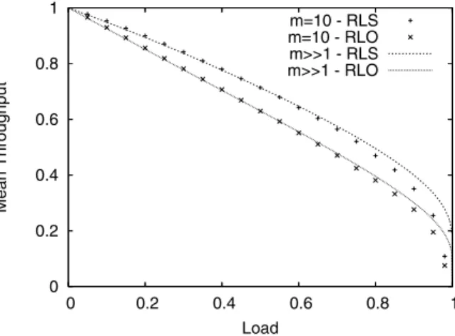
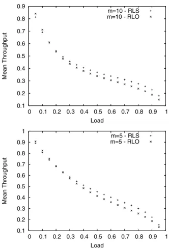
servers. We then study open systems where clients arrive according to a random process and leave the system upon service completion. In this scenario, we ana- lyze how client migrations within the system interact with the system dynamics induced by client arrivals and departures. We compare the load-aware RLS strat- egy to a load-oblivious strategy in which clients just randomly switch server with- out accounting for the server loads. Surprisingly, we show that both load-oblivious and load-aware strategies stabilize the system whenever this is at all possible. We use large-system asymptotics to characterize system performance, and augment this with simulations, which suggest that the average client sojourn time under the load- oblivious strategy is not considerably reduced when clients apply smarter load-aware strategies.

Keywords Mean field asymptotics · Stability analysis

Mathematics Subject Classification 60K25 · 68M14 · 68M20

1 Introduction

Load balancing is a key component of today’s communication networks and com- puter systems in which resources are distributed over a wide area or across a large number of systems and have to be shared by a large number of users. Load balanc- ing enables efficient resource utilization and thereby tends to improve the quality of service perceived by users. Traditionally, load balancing has been achieved by ap- plying smart routing policies: when a new demand arrives, it is routed towards a particular resource depending on the current loads of the various resources; see [14]

and references therein. In contrast, we are interested in systems where a new task is initially assigned to a resource chosen at random irrespective of the current re- source loads, but where tasks can be re-assigned, i.e., migrate from one resource to another.

Our primary motivation stems from the increasing popularity of Dynamic Spec- trum Access (DSA) techniques [1] as a potential mechanism for broadband access in future wireless systems. A common implementation platform for DSA is the use of reprogrammable Software-Defined-Radios (SDRs). These new radios are frequency- agile or flexible, and have the ability to rapidly jump from one frequency band to another in order to explore and exploit large parts of the spectrum. A central ques- tion in DSA is how multiple users may fairly and efficiently share spectrum in a distributed manner. Typically, the service rate of a user on a given frequency band is inversely proportional to the number of users transmitting on this band, i.e., to the load of the band. As new users entering the system have no way of determining the load on each frequency band, they have to initially select a band randomly. Should a user receive a quite poor quality of service on a given band, she may resample a new band at random and decide to switch to it. The overall system performance then strongly depends on the distributed resampling and switching strategy implemented by each user.

Though our primary motivation is DSA, our methods and results could provide

insight into a number of other applications. One such pertains to wireline networks,

where there has recently been interest in multipath routing [15]. Here, users may use several path to download files, and have to select the appropriate path or the set of paths. Another application is in transport networks, where one might wish to un- derstand how Wardrop equilibria, which correspond to the equalization of journey times across alternative routes, are achieved or approximated by network users act- ing on limited information. Our results could also shed insight on how quickly such equilibria can be re-established following major disruptions or other changes to the network. Finally, note that distributed load resampling can also be thought of as a game between selfish users. In fact, it is an instance of a congestion game (see, for example, [18]), and our results shed light on the time to reach a Nash equilibrium in such a game, but it also helps understanding the outcome of the game with a dynamic population of players.

We consider a generic system consisting of multiple servers (in DSA, frequency bands) employing the Processor Sharing (PS) service discipline, shared by clients who have to initially pick a server at random, and may later resample servers and mi- grate during their service. We restrict our attention to two natural distributed resam- pling and migration strategies, the Random Local Search (RLS) and Random Load- Oblivious (RLO) strategies. When implementing the RLS algorithm, a user resamples a new randomly chosen server at the instants of a Poisson process, and migrates to this new server if its load is smaller than that of the initial server. In contrast, under the RLO algorithm, a user hops between servers according to a random Markovian jump process irrespective of the loads of the visited servers.

We investigate both closed systems with fixed population of clients, and open systems with a population whose dynamics are governed by client arrivals and the completions of their services. In closed systems, we are interested in characterizing the time that it takes under the RLS algorithm to balance all server loads (note that here the RLO algorithm does not balance loads except in an average sense—so we do not study this algorithm in closed systems). In open systems, users arrive at the various servers according to independent stochastic processes of fixed intensities, and leave upon service completion. In this scenario, client migrations within the system interact in a complicated manner with the system dynamics induced by client arrivals and departures. We aim at characterizing system stability under the RLS and RLO strategies, as well as at deriving estimates of user sojourn times. Our contributions are as follows:

• Closed systems. We show that, starting from an arbitrary allocation of users to servers, the time τ it takes to achieve perfect balance of server loads (the system reaches perfect balance if the number of users at any pair of servers differs by at most 1) scales at most as log(m)(

+ log(m)), where m and n denote the num- ber of servers and users, respectively. This is a considerable improvement over the existing bounds that stated that τ scales at most as m

(see, for example, [12]). We also investigate the time τ

to reach an approximate -balance (a system reaches an approximate -balance if there exists p such that the number of users associated to any server lies between (1 − )p and (1 + )p). We show that τ

scales at most as log(m)/.

• Open systems. We demonstrate that both RLS and RLO strategies achieve the

largest stability region possible, i.e., that the system is stable under these two algo-

rithms provided that

i=1

λ

<

i=1

μ

, where λ

denotes the initial user arrival rate at server i and μ

is the service rate of this server. The result is not surpris- ing for RLS, but less intuitive for RLO since, under this algorithm, users take no account of server loads when migrating. For both RLS and RLO strategies, we derive approximate estimates of the average user sojourn time using large- system asymptotics. The estimates are shown to be exact when the number of servers grows large, but turn out to be quite accurate for systems of limited sizes as well. Our first numerical results suggest that again, surprisingly, the average client sojourn time under the load-oblivious RLO strategy is not considerably reduced when clients apply smarter load-aware RLS strategy. To our knowledge, this pa- per is the first to analyze the performance of RLS and RLO algorithms in open systems.

The paper is organized as follows. We describe our model and notation in Sect. 2, and related work in Sect. 3. Sections 4 and 5 are devoted to the analysis of closed and open systems, respectively. We provide concluding remarks in Sect. 6.

2 Model description and notation

We consider a set of m Processor Sharing servers of respective capacities μ

, . . . , μ

. The system is homogeneous if μ

= 1 for all i = 1, . . . , m. The system state at time t is represented by the number of clients associated to each server, N (t ) = (N

(t ), . . . , N

(t )). The service rate of a client associated to server i at time t is then μ

/N

(t ). Clients independently resample and switch servers to selfishly im- prove their service rate. They have a myopic view of the system in the sense that they are aware of their current service rates, but do not know the service rate they would achieve at other servers. Given this myopic view, it is natural to consider and analyze the two following random distributed resampling and migration algorithms:

• Random Local Search (RLS) algorithm. At the instants of a Poisson process of in- tensity β > 0, a client picks a new server uniformly at random and migrates to it if and only if this would increase her service rate. In other words, if at time t , a client associated to server i picks server j , she migrates to j if and only if μ

/(N

(t ) + 1) > μ

/N

(t ).

• Random Load-Oblivious (RLO) algorithm. After arriving in the system, each client visits successive servers according to a continuous-time random walk with transi- tion matrix Q = { q

, i, j = 1, . . . , m } . The random walks are independent across clients, and irreducible. We denote by π the stationary distribution of this random walk. Note that as a consequence of irreducibility, clients visit all servers eventu- ally, i.e., π

> 0 for all i = 1, . . . , m.

Note that under the RLO algorithm, clients do not take loads into account when

switching servers. In particular, they may move to a server with a higher load. An

example of such a resampling strategy is as follows. Each client has a Poisson clock

of rate β > 0 and, when her clock ticks, she picks a new server uniformly at random

and moves there irrespective of its load.

We analyze the performance of distributed resampling and migration strategies in closed and open systems. In closed systems, the total population of clients is fixed, equal to n. There are no arrivals or services. Such systems can be thought of as mod- elling persistent clients, who remain in the system forever (relative to some appro- priate time-scale), and derive utility which is greater if their ‘share’ of a server (the reciprocal of the total number of clients at that server) is greater. For such systems, we investigate the time it takes under the RLS algorithm to balance clients across servers, starting from any arbitrary system state. In open systems, exogenous clients associate to server i according to a Poisson process of intensity λ

(the arrival processes are independent across servers). Client service requirements are i.i.d. exponentially dis- tributed with unit mean. Under RLS and RLO algorithms, (N (t ), t ≥ 0) is a Markov process. In open systems, we are interested in characterizing the stability region of RLS and RLO strategies, defined as the set of arrival rates λ = (λ

, . . . , λ

) such that the system is stable, i.e., such that (N (t ), t ≥ 0) is positive recurrent. We also aim at estimating the average client sojourn time.

3 Related work

There have been many studies on distributed, selfish load balancing algorithms and routing games in closed systems; e.g., [16] and references therein. Refer to [18] for a quite exhaustive survey. Much of the work in this area has concentrated on finding the fastest sequence of moves that would balance the system, also called Nashification [11]. One class of algorithms is the elementary step system, first described in [19] in which a sequence of best response moves are performed by the clients. Of course, this requires that the clients know the status of all the other servers. In [4, 5], the authors study closed systems with limited information about the servers’ status. They consider a synchronous system where at each step, each server samples a new server randomly and if the load of the sampled server is smaller, then a client moves with probability (N

− N

)/N

, where N

is the load on the current server and N

is the load of the sampled server. It is shown that the expected time to balance the system is O(log log m + n

). A modification of this load balancing algorithm is studied in [5], and it is shown that the expected time to balance the system is O(log m + n log n).

In [12], the author considers clients dynamics identical to those considered in this paper and uses the potential function introduced in [10] to quantify the time to achieve system balance. It is shown that the expected time to reach a balance scales at most as O(m

). We provide significant improvements on this bound.

In open systems, the client moves interact in a complicated manner with the client arrival and departure processes. There is very little work trying to understand this interaction. None of the existing work deals with a system similar to that studied here.

For instance, [2] analyzes the interaction in a game-theoretical framework, where

arrivals are adversarial, and where a central controller moves clients with the aim of

stabilizing the system. The performance of the classical work stealing load-balancing

scheme has also been studied; see, for example, [3] and references therein. Of course,

there is an abundant literature on the performance of classical load-balancing schemes

in open systems where clients are assigned to a given server for the entire duration

of their service; see, for example, the analysis of the supermarket model in [13, 17].

To our knowledge, the present paper provides the first analysis of natural distributed resampling and migration strategies in open systems.

4 Closed systems

In this section, we analyze the performance of the RLS resampling strategy in a closed homogeneous system, and obtain tight bounds on the expected time to balance the server loads.

Recall that there are n clients distributed among m servers. Let n = qm + r, 0 ≤ r ≤ m − 1. We now define the following:

• The state N (t ) = (N

(t ), . . . , N

(t )) is balanced if |N

(t ) − N

(t )| ≤ 1 for 1 ≤ i < j ≤ m. The time to balance, τ , is defined as

τ := inf

t > 0 : N (t ) is balanced .

• The state N (t ) is -balanced if (1 − )p ≤ N

(t ) ≤ (1 + )p for all i = 1, . . . , m, where p = n/m. The time, τ

, to -balance is defined as

τ

:= inf

t > 0 : N (t ) is -balanced .

Let f, g : N → R

. We say f (k) = O(g(k)) if there exists c ∈ R

such that f (k) ≤ cg(k) for all k. Similarly, for f, g : N

→ R

, we say f (k, l) = O(g(k, l)) if there exists c ∈ R

such that f (k, l) ≤ cg(k, l) for all k and l.

4.1 Time to reach balance

We now characterize the time required by the RLS algorithm to reach perfect bal- ance and -balance. Throughout, we shall consider a sequence of systems indexed by (m, n), the number of servers and clients, respectively. Our results apply if either of these tend to infinity along the sequence, but in practice we shall be interested in the case when both are large, which is captured by an asymptotic regime in which both quantities tend to infinity.

In practice, interest focuses on the case where n ≥ m, i.e., there are more clients than servers and balancing the load is important because servers are a valuable re- source. In the lightly loaded case of there being more servers than clients (m > n), load balancing may not be as important. Nevertheless, for completeness, we also treat this case.

Suppose first that m ≥ n along the sequence. Then, in a balanced configuration, every server will have 0 or 1 clients at it. (In this case, -balance can be more demand- ing than perfect balance, and hence impossible! So we only consider perfect balance.) The problem of reaching such a configuration from an arbitrary initial configuration is related to the coupon collector problem, which has been extensively studied.

Lemma 1 Suppose that the number of servers, m, is no smaller than the number

of clients, n. Then, the expected time, E[ τ ], for randomized local search to achieve

balance is O(

log n).

In the remainder of this section, we shall focus on the more practically relevant case, where there are more clients than servers.

Theorem 1 Consider a sequence of systems indexed by (m, n), and suppose that n > m along this sequence. The expected time, E[ τ ] , for randomized local search to achieve balance is O(log(m)(

+ log(m))).

Theorem 2 Consider a sequence of systems indexed by (m, n), and suppose that n > (1 + α)m along this sequence, for some constant α > 0. The expected time, E[ τ

] for randomized local search to achieve -balance is O(log(m)/).

Remarks

1. It is easy to see, applying Markov’s inequality, that the same upper bounds on the time to balance hold in probability as in expectation.

2. We now compare our bounds on τ with that from [12]. From Theorem 2.7 of [12], the expected number of attempted moves before reaching balance is O(m

n).

Since move attempts (resampling) occur at rate n, this gives us a time complexity of O(m

). Our bound in Theorem 1 is much tighter.

3. Our bound is close to the best possible. To see this, suppose m divides n exactly.

At some stage, the algorithm will reach an allocation in which one server has n/m + 1 clients, one other server has n/m − 1 clients and all others have exactly n/m clients. Each of the n/m+1 clients at the overloaded server attempts to move at rate 1, and each move attempt is successful with probability 1/m. Hence, the mean time for just the final move is m

/(m + n) ≥ m

/(2n). Our bound is only a log m factor higher than the time for the last move.

Alternatively, consider the situation when m

= o(n) and all n clients are ini- tially at the same server. Then, at least n − n/m clients need to move out of this server to reach balance. When there are k clients at the server, the expected time to the next move is at least 1/ k (possibly more, as the move attempt may not be successful). Hence, the expected time to reach balance is at least

1 k ≥

n/m

1

x dx = log m.

Again our bound is only a log m factor higher than the above lower bound on the time to reach balance.

4.2 Proofs

Without loss of generality, we take the rate β of the independent Poisson clocks at

each client to be unity. A client at server i whose clock has ticked at time t attempts

to move by sampling a server uniformly at random from all m servers. It moves to

the sampled server, say j , if and only if N

(t ) − N

(t ) > 1. Clearly, N (t ) evolves as

a continuous time Markov chain.

4.2.1 Proof of Lemma 1

Recall that every server has 0 or 1 clients in a balanced configuration. Assume we don’t start with a balanced configuration, and consider some time t < τ , when the configuration is still unbalanced. Let A

(t ) denote the number of empty servers, and A

(t ), i ≥ 1 the number of servers with exactly i clients. Then, A

(t ) ≥ m − n + 1, and

τ = inf

t ≥ 0 : A

(t ) = m − n . Noting that A

(t ) +

i=1

A

(t ) = m, while

i=1

iA

(t ) = n, we conclude that the number of clients at servers with two or more clients is given by

iA

(t ) = n − A

(t ) ≥ n − m + A

(t ). (1) Each of these clients attempts to move at unit rate, independent of other clients. If it chooses an empty server to move to, then the number of empty servers decreases by 1.

Define T

= inf{ t ≥ 0 : A

(t ) ≤ k } to be the first time that the number of empty servers is no more than k. When the number of empty servers hits m − n, the system is balanced; in other words, τ = T

.

The random time, T

− T

, for A

(t ) to decrease from k to k − 1, is stochastically dominated by an exponential random variable denoting the time for one of the clients in servers containing two or more clients to move to an empty server. By (1), the number of clients at such servers is at least n − m + k at time T

. Each of these moves at rate 1, and chooses an empty server to move to with probability k/m. Hence,

T

− T

Exp

k(n − m + k) m

,

where we write X Y to mean that X is stochastically dominated by Y . We shall also write Exp(λ) to denote an exponential random variable with parameter λ and mean 1/λ. It follows that

E[ T

− T

] ≤ m

k(n − m + k) = m m − n

1

k + n − m − 1 k

. (2)

We also note that A

(t ) is monotone decreasing in t , and that A

(0) ≤ m − 1. Hence, E[ τ ] = E[ T

] ≤

m

E[ T

− T

]

≤ m m − n

m

1

k + n − m − 1 k

≤ m m − n

1 +

m−n+1

1 x + n − m dx

= m

m − n 1 + log(n − 1) .

This completes the proof of the lemma.

4.2.2 Proof of Theorem 1

Define V (t ) := max

N

(t ), i.e., V (t ) is the maximum number of clients associ- ated with any server at time t . Define C

(t ) to be the number of servers with exactly v clients, B

(t ) to be the number with exactly v − 1 clients and A

(t ) to be the number with strictly less than v − 1 clients, all at time t .

The idea of the proof is as follows. The evolution of N (t ) towards balance is divided into phases. If V (t ) = v, then N (t ) is said to be in phase v. Thus, C

(t ) is the number of maximally loaded servers in phase v. Since a client never moves to a server that has more clients than its current server, V (t ) is monotone decreasing and, in each phase, C

(t ) is also monotone decreasing. Phase v ends when C

(t ) = 0. Let τ

denote the (random) length of phase v. Each phase can be further divided into sub-phases, say (v, c), when C

(t ) = c. Let τ

denote the random length of time that it takes for C

(t ) to decrease from c to c − 1. Observe that τ

=

c

τ

and τ =

v

τ

. When N (t ) is balanced, V (t ) =

, C

m

(t ) = r if r > 0 and C

m

(t ) = m otherwise. This gives us the maximum range for v. The number of sub-phases in each phase is also similarly bounded. The theorem is proved by bounding the expected times of each of the sub-phases and phases.

Proof In phase v, observe that

vC

(t ) + (v − 1)B

(t ) ≤ n, m − B

(t ) − C

(t ) = A

(t ).

Furthermore, if N (t ) is not balanced, then there has to be at least one server with v − 2 or fewer clients (i.e., A

(t ) ≥ 1). Hence, while the system is unbalanced, we have

A

(t ) ≥

⎧ ⎨

⎩

m −

, v ≥

+ 1, 1, v ≤

.

(3) Each of the vC

(t ) clients at one of the maximally loaded servers samples one of the m servers at random at unit rate. If the sampled server happens to be one of the A

(t ) servers with v − 2 or fewer clients, then the client moves to the sampled server and C

(t ) decreases by 1. This event has probability A

(t )/m. Hence, C

(t ) decreases by 1 at rate vC

(t )A

(t )/m, and we obtain from (3) that

τ

˜ τ

∼ Exp(λ

), where λ

=

⎧ ⎨

⎩

vc 1 −

, v ≥

+ 1,

vc

m

, v ≤

.

(4)

Here we write X ∼ Y to mean that the random variables X and Y have the same distribution. In particular,

E[ τ

] ≤ E[ ˜ τ

] =

⎧ ⎨

⎩

1 vc

m(v−1)

[m(v−1)−n]

, v ≥

+ 1,

m

vc

, v ≤

.

(5)

At any time t, C

(t ) is bounded above by n/v , since there cannot be more than this many servers with v clients. Since phase v ends when C

= 0, we have E[ τ

] ≤

c=1

E [ τ

], and we obtain using (5) that E[ τ

] ≤

⎧ ⎨

⎩

m(v−1) v[m(v−1)−n]

1

c

, v ≥

+ 1,

m v

1

c

, v ≤

.

(6) Moreover, for all v ≥

, we readily see that,

1 c ≤ 1 +

1

1 x dx

≤ 1 + log n

v ≤ 1 + log m.

Hence, we can rewrite (6) as E[ τ

] 1 + log m ≤

⎧ ⎨

⎩

m(v−1)

v[m(v−1)−n]

, v ≥

+ 1,

m

v

, v ≤

.

(7)

Finally, the time τ it takes to reach perfect balance satisfies τ ≤

τ

+

τ

. (8)

Now, we have by (5) that E[ τ

] ≤

, and so,

c=r+1

E[ τ

] ≤ m n/m

1 c

≤ m

n

1 +

1

1 x dx

= m

n (1 + log m). (9)

Hence, from (7), (8), and (9), we obtain E[ τ ]

1 + log m ≤ m

n +

n/(m

m v

+

m

m(v − 1) − n . (10)

The number of terms in the first sum above is at most max{1,

}. Each summand

is no more than m

/n. Hence, the first sum is bounded above by max{

, 2}. The

second sum is bounded above by m

mn m−1

− n +

m−1n +1

m

m(x − 1) − n dx = m(m − 1)

n + log m(n − 1) − n

mn

m−1

− n . Substituting these expressions in (10) and simplifying, we get

E[ τ ] ≤ (1 + log m)

max m

n , 2

+ m

n + log m

+ m

n

≤ 3(1 + log m) m

n + log m + 1

.

This completes the proof.

4.2.3 Proof of Theorem 2

Recall that p = n/m. We need the following definitions.

– Server i is -balanced at time t if (1 − )p ≤ N

(t ) ≤ (1 + )p, underloaded if N

(t ) < (1 − )p and overloaded if N

(t ) > (1 + )p. M

(t ), M

(t ), and M

(t ) denote the number of -balanced, underloaded, and overloaded servers, respec- tively.

– The underflow from server i is defined to be u

(t ) =

0 if N

(t ) ≥ p, p − N

(t ) otherwise.

Also, let U (t ) :=

i=1

u

(t ). Similarly, define the overflow from server i as o

(t ) =

0 if N

(t ) ≤ p, N

(t ) − p otherwise, and O(t ) :=

i=1

o

(t ).

Proof Let N

(t ) be the number of ‘overflowing’ clients defined as N

(t ) :=

i∈MO(t )

N

(t ) − (1 + )p ,

where M

(t ) is the set of overloaded servers at time t. We can write U (t ) ≤ M

(t ) × p

+ M

(t ) × (p), O(t ) ≥ N

(t ) + m − M

(t ) − M

(t )

× (p).

Since O(t ) = U (t ), we obtain

pM

(t ) + (p)M

(t ) ≥ N

(t ) + m − M

(t ) − M

(t )

(p),

which yields

N

(t ) ≤ p M

(t ) + M

(t ) (1 + ) − m M

(t ) + M

(t ) ≥ N

(t )

(1 + )p + 1 + m

≥ max

N

(t ) (1 + )p ,

1 + m

.

Now consider a client that is attempting to move at time t . We say that this attempt results in a good move if the attempt results in a migration that reduces N

(t ). Let G denote the event corresponding to a good move. When the state of the system is (N

, M

, M

), the probability of a good move is

P (G) ≥ N

+ (1 + )p n

M

+ M

m ,

and the number of attempts between successive good moves is geometric with mean at most

O+p)MU

.

Let K

denote the number of attempts before a good move occurs from the state (N

, M

, M

). The expected number of attempts before a good move reduces N

satisfies

E[ K

] ≤ mn

(N

+ (1 + )p)(M

+ M

) .

Let K

denote the number of attempts to achieve -balance. In the worst case, N

(t ) starts at (m − 1)p and ends at 1. We can then bound E[ K

] as follows:

E[ K

] ≤

(m−

mn ((1 + )p + i) max

(1+)p

,

m

=

mn

((1 + )p + i)

m +

(m

mn

((1 + )p + i)

= 1 +

n

1 ((1 + )p + i) + mn

(m−

1

i − 1

((1 + )p + i)

≤ 1 + n log

(1 + )p + n (1 + )p

+ mnlog

(m − 1)p n

(1 + )p + n (1 + )p + (m − 1)p

≤ n

log(1 + m) + mn

− 1

m + 1 +

m −

m

≤ n log(m).

Since each client is sampling at unit rate, the total sampling rate is n and the average time to reach -balance, E[ τ

] is E[ K

] /n. Thus E[ τ

] = O((log m)/).

5 Open systems

In open systems, we are interested in quantifying classical queueing performance metrics, such as the stability region and the mean client sojourn time. We first inves- tigate the stability region achieved under RLO and RLS algorithms. Both algorithms are shown to stabilize the system whenever this is at all possible, which for load- oblivious RLO algorithm may be surprising. Then, we try to obtain more detailed estimates of the system performance. As it turns out, the system equilibrium distribu- tion is difficult, if not impossible, to derive, and we rely on large-system asymptotics to provide insights into the way the system behaves.

5.1 Stability

In the following, we denote λ = (λ

, . . . , λ

) and μ = (μ

, . . . , μ

) the vectors representing the arrival and departure rates at the various servers. · denotes the L

-norm on R

. We first provide an upper bound on the maximum stability region defined as the set of λ such that there may exist a resampling and migration strategy stabilizing the system. This set is obtained by assuming that all servers’ resources are pooled.

Proposition 1 Assume that λ is such that

i

λ

>

i

μ

. Then there is no resam- pling and migration strategy stabilizing the system.

Proof The proof is straightforward. Remark that for any resampling and migration strategy, the total service rate is less than

i

μ

. Then if

i

λ

>

i

μ

, the average number of clients in the system grows at a rate greater than

i

λ

−

i

μ

> 0. The

system is then unstable.

The two following theorems state that both RLO and RLS strategies achieve max- imum stability.

Theorem 3 Assume that

i

λ

<

i

μ

. Then the system is stable under RLO algo- rithm.

Theorem 4 Assume that

i

λ

<

i

μ

. Then the system is stable under RLS algo- rithm.

A result somewhat similar to that of Theorem 3 was first stated in [7] using heuris-

tic fluid limits arguments. Fluid limits are powerful techniques to study ergodicity

of Markov processes [8]. They comprise the study of the system behavior in the following limiting regime: the initial condition is scaled up by a multiplicative fac- tor k, time is accelerated by the same factor, and k tends to ∞ . Often the system becomes tractable in this regime and even deterministic. If the system in the fluid regime reaches 0 in a finite time, then the process is ergodic. In the fluid regime, clients stay for very long periods of time in our system, and since, under RLO al- gorithm, the client random walks are ergodic, the probability that a given client is associated to server i should be proportional to π

(the equilibrium distribution of the random walk). In such case, when the client population is large (as in the fluid regime), all servers should be occupied and active, ensuring that the system empties in finite time. This is the argument used in [7], but not justified. The problem arises because the client migration process actually interacts with arrivals and departures.

Handling this interaction turns out to be extremely difficult. Recently however, in [21], the authors were able to formally derive the system fluid limits, and analyze its stability under very specific assumptions on the client random walk (its transition matrix Q has to be diagonalizable). Their proof is quite intricate. In the following, we prove Theorem 3 without the use of fluid limits, and for any random walk. Our proof is much more direct than that in [21], and hence is amenable to deal with more general cases and possible extensions. For the proof of Theorem 4, we use a rather classical method, namely, we exhibit a simple Lyapunov function.

5.1.1 Proof of Theorem 3

Recall that by definition, under RLO strategy, the process (N (t ), t ≥ 0) is the Markov process with the following non-zero transition rates for 1 ≤ i = j ≤ m:

⎧ ⎪

⎨

⎪ ⎩

Ω(n, n + e

) = λ

, Ω(n, n − e

+ e

) = n

q

, Ω(n, n − e

) = μ

1

,

(11)

where n = (n

, . . . , n

) ∈ N

and e

is the m-dimensional vector with every coordi- nate equal to 0, except for the ith one equal to 1. The matrix Q = (q

) describes the migration of clients, and it is only assumed to possess a unique stationary distribution π = (π

) such that π

> 0 for each i = 1, . . . , m. The aim of the analysis is to use the following result, known as Foster’s criterion [20].

Foster’s criterion If there exist K and t ≥ 0 such that sup

n∈N^m:n≥K

E

N (t ) − n

< 0, (12)

where E

( · ) = E ( ·| N (0) = n), then (N (t ), t ≥ 0) is ergodic.

Kolmogorov’s equation is the first step that leads to (12): for any t ≥ 0, the drift E

(N (t ) − n) is given by

E

N (t ) − n

= λ t −

0

E

i=1

μ

1

du.

This gives the following inequality, which is the basis of our drift analysis:

E

N (t ) − n

≤ λ t − μ

0

P

N (u) > 0

du, (13)

where P

[·] = P[·| N (0) = n ] , and for x ∈ N

, x > 0 is to be understood coordinate- wise, i.e., x

> 0 for each i = 1, . . . , m.

The idea of the proof of (12) is that when the system starts with many clients, then the number of arrivals and departures is negligible on the time interval [0, t ] and the system behaves like the closed one. For a closed system, it is not difficult to show, using the fact that Q has an invariant measure, that P (N (u) > 0) for u > 0 is arbitrarily close to 1 as the number of clients in the system increases. In view of (13), this gives a negative drift when

i

λ

<

i

μ

.

The following coupling initially proposed and formally justified in [21] is key to relate the open and closed systems. For n ∈ N

and , ρ ∈ R

, denote by N

the process under RLO strategy starting in the initial state n, with arrival rate

at server i with capacity ρ

. Then (N

(t )) is the Markov process with N

(0) = n, and with non-zero transition rates given by (11) with

instead of λ

and ρ

instead of μ

. Then the processes N

and N

can be coupled in such a way that for some process Z(t ) ≥ 0,

N

(t ) = N

(t ) − N

(t ) + Z(t ), t ≥ 0.

Moreover, the processes N

and N

are independent, and N

is a Poisson process with parameter ρ . Essentially, this coupling realizes the process N

with arrivals and departures as the difference between two processes without departures.

This coupling can be constructed as follows: consider a particle system with three kinds of particles, colored blue, red, and green. All the particles in the system are performing independent continuous-time random walks, going from i to j at rate q

, and the system starts with only blue particles.

Consider two independent Poisson processes N and N

with respective parame- ters and ρ : at times of N , add a new blue particle at server i with probability

i

/ . At times of N

, consider server i with probability ρ

/ ρ : if there is a blue particle, choose one at random and turn it into a red one. If there is no blue particle, add a green particle.

If B

(t ), R

(t ), and G

(t ) are respectively the number of blue, red, and green par- ticles at server i at time t , then it is easy to see that:

– B is distributed like N

, – B + R is distributed like N

,

– R + G is distributed like N

and B + G = N

is independent of B + R.

This proves the coupling with Z(t ) = G(t ). The process N

can be seen as the superposition of the initial particles with the particles arriving at rate , hence the additional coupling N

= N

+ N

holds, and finally, N

can be written

N

(t ) = N

(t ) + N

(t ) − N

(t ) + Z(t ), t ≥ 0,

with N

and N

independent, and Z(t ) ≥ 0. Starting from (13), we now turn our attention to proving the existence of constants K and t which satisfy (12). We have, using the coupling’s notation, P

(N (u) > 0) = P (N

(u) > 0) and hence, for any 0 ≤ u ≤ t and n ∈ N

,

P

N (u) > 0

= P N

(u) + N

(u) + Z(u) > N

(u)

≥ P N

(u) > N

(u) .

Since the process N

is independent of the random variable N

(t ) , we can work conditionally on the value of N

(t ) and study the quantity P (N

(u) > M).

Thus we only need to consider the closed process N

henceforth, and so we simplify the notation and note N

= N

. Markov’s inequality gives

P ∃ i ∈ {1, . . . , m } : N

(u) ≤ M

= 1 − P N

(u) > M

≤

P N

(u) ≤ M

≤ e

E e

.

For any i ∈ {1, . . . , m },

E e

=

E

e

where ξ under P

is a continuous-time Markov chain with transition rates Q = (q

), and which starts at ξ(0) = j . If p(j, i, u) = P

(ξ(u) = i), one gets for u ≥ t

> 0 and n ∈ N

with n ≥ K

E e

= e

m

j=1njlog(1−(1−1/e)p(j,i,u))

≤ e

≤ e

with p(t

) = inf

min

p(j, i, u). Note that since, for any 1 ≤ i, j ≤ m, p(j, i, u) > 0 for any u > 0 and p(j, i, u) → π

> 0 as u → +∞ , one has that p(t

) > 0. Therefore, for u ≥ t

and n with n ≤ K, integrating with respect to the law of N

(t ) gives

P N

(u) > N

(t ) ≥ 1 − ε(t, K, t

) with ε(t, K, t

) = me

. In particular, for t ≥ t

,

sup

n∈N^m:n≥K

E

N (t ) − n

≤ λ t − μ (t − t

) 1 − ε(t, K, t

) .

Since by assumption λ < μ , it is not difficult to choose constants t, t

, and K

such that the right hand side is strictly negative (for instance, t = 1, t

small enough,

and K large enough), which gives the result.

5.1.2 Proof of Theorem 4

Intuitively, it is clear that the load-dependent RLS strategy performs better than the load-oblivious RLO policy, since it seems harder under RLS to see an empty server.

This simple observation shows that the number of empty servers should be part of a Lyapunov function, and indeed this leads us to define the function f : N

→ R

by:

∀ n, f (n) =

max(, n

) = n + εk

(n)

with k

(n) = 1

+ · · · + 1

the number of empty servers in state n. In order for f to be a Lyapunov function, the constant 0 < < 1 has to satisfy

×

i

μ

<

i

(μ

− λ

) − γ for some γ > 0.

Let K

(n) (resp., K

(n)) be the set of servers that are empty (resp., have a single client). Denote by k

(n) and k

(n) the respective cardinalities of these sets. Let us compute the average drift f (n) of the Markov process N (t ) under RLS strategy.

We have

f (n) =

i

λ

−

i /∈K0(n)

μ

+

i∈K1(n)

μ

−

i∈K0(n)

λ

− Y (n)

,

where Y (n) is the rate in state n at which empty servers are fed by migrating clients.

– If k

(n) = 0, there are no empty servers in state n and in particular Y (n) = 0. We have

f (n) =

i

(λ

− μ

) +

i∈K₁(n)

μ

< − γ because of our choice of .

– If k

(n) > 0, there is at least one empty server in state n. Define p(n) = max

n

. Considering migrations of the p(n) clients from (one of) the server(s) with max- imum size to one of the empty servers, we obtain Y (n) ≥

, which ensures that f (n) < − γ when p(n) is large enough, say greater than K.

We conclude the proof by considering the drift outside the set F = { n : f (n) <

m(K + ) }. First, remark that F is finite. Then, when n / ∈ F , p(n) ≥ K. We deduce that for all n / ∈ F : f (n) < − γ . The positive recurrence follows.

5.2 Approximate performance estimates

The system behavior in stationary regime under RLO and RLS strategies is extremely

difficult to analyze. For example, (N (t ), t ≥ 0) is unfortunately not reversible under

these strategies. To obtain estimates of the steady state distribution and client so- journ times, we use large-system asymptotics, i.e., we let m grow large. Recently, large-system asymptotics have been successfully applied in many contexts in com- munication systems. They have been used, for example, to understand load balancing issues such as those arising in the supermarket model [13, 17, 23]. In the rest of the section, we denote by N

(t ) the vector representing the numbers of clients at time t at each server in a system with m servers under either RLO or RLS algorithm.

In what follows, we consider homogeneous systems where λ

= λ and μ

= 1 for all i. This restriction simplifies the notation and results, but is not essential. We discuss at the end of this subsection how to deal with heterogenous systems. We also assume that the number of clients associated to a given server is bounded by a (possibly very large) constant B . Again this assumption is not crucial, but relaxing this assumption would require a much more involved analysis, as explained below.

5.2.1 RLO algorithm

We first consider RLO algorithms. We assume that a client jumps from one server to another at the instants of a Poisson process of intensity β, and that the next server is chosen uniformly at random. The analysis can be extended to any random walk (see Sect. 5.2.3). We represent the system state at time t by X

(t ) the proportion of servers with exactly k clients at time t. We also define S

(t ) =

l≥k

X

(t ).

Let us compute the average change in the system state in a small interval of time of duration dt , and more specifically the change in X

. Arrivals occur at rate λm: An arrival increases X

if it occurs at servers with k −1 clients, and decreases X

if it occurs at servers with k clients. Hence the change in X

due to exogenous arrivals is dt λ(X

− X

). Departures can be analyzed similarly. Let us now compute the change due to client migrations. Clients migrating to server with k − 1 (resp., k) clients increase (resp., decrease) X

. In addition, clients migrating from servers with k (resp., k + 1) clients decrease (resp., increase) X

. The average change in X

due to client migrations is thus dtβ((X

− X

)

j

j X

− kX

+ (k + 1)X

). In summary, the average change in X

during dt is

dt ×

λ X

− X

− X

− X

+ β X

− X

j

j X

− kX

+ (k + 1)X

.

There is no explicit dependence on m, and hence we expect the dynamics of X

(t ) to be close to those of a deterministic solution x

of the following sets of differential equations: for all k ∈ {0, . . . , B },

˙

x

= λ(x

− x

) − (x

− x

) + β

(x

− x

)

j

j x

− kx

+ (k + 1)x

, (14)