Acoustic navigation for the autonomous underwater vehicle REMUS

Acoustic Navigation for the Autonomous

Underwater Vehicle REMUS

by

Thomas F. Fulton

B.Sc., Ocean Engineering

United States Naval Academy, Annapolis Maryland (1992)

Submitted to the Department of Ocean Engineering

in partial fulfillment of the requirements for the degree of

Master of Science in Ocean Engineering

at the

MASSACHUSETTS INSTITUTE OF TECHNOLOGY

June 2000

©

Massachusetts Institute of Technology 2000. All rights reserved.

Author ...

Department of Ocean Engineering

May 5, 2000

Certified by...

Accepted

...-John J. Leonard

Assistant Professor of Ocean Engineering

Thesis Supervisor

b y . . . .. .. ... .. .. 7. ... .... ... .. I ...

Professor Nicholas Patrikalakis

Kawasaki Professor of Engineering

Chairman, Departmental Committee on Graduate Students

MASSACHUSETTS INSTITUTE OF TECHNOLOGY

Acoustic Navigation for the Autonomous Underwater

Vehicle REMUS

by

Thomas F. Fulton

Submitted to the Department of Ocean Engineering on May 5, 2000, in partial fulfillment of the

requirements for the degree of Master of Science in Ocean Engineering

Abstract

The requirement for autonomous operation of Underwater Vehicles has led to several methods of navigation. One of the primary methods for navigation is Long Base-Line (LBL), where prepositioned acoustic transponders are used for a vehicle to find its own position. Due to vagaries of the acoustic path and difficulty in recognizing the direct path signal arrival, relying solely on acoustic transponder data results in navigation errors. These errors preclude an AUV from obtaining navigation accuracy better than a few meters over an operating area of several kilometers. By imple-menting an Extended Kalman Filter (EKF), vehicle state information is incorporated to the navigation solution, yielding an improved navigation fix over acoustic data alone. The future work in this area is in autonomous decision making for naviga-tion. By taking out the 'man-in-the-loop', true autonomous operation is achieved, and the benefits of AUVs will be realized. This thesis examines the performance of our EKF, which uses the state data of heading and speed to improve acoustic fixes. The performance is illustrated by two methods. First, navigation data from missions at LEO-15, off the coast of New Jersey in July 1999, are post-processed using an EKF. Second, in-water experiments were conducted in Buzzards Bay, Woods Hole MA in April 2000, utilizing an on-line EKF. The results demonstrate the potential for smoother trajectory estimation, however reveal the potential sensitivity to EKF divergence when navigating in an array with only two transponders. This method is then evaluated as a springboard to autonomous decision making by the AUV. Thesis Supervisor: John J. Leonard

Acknowledgments

This thesis is the culmination of two years of work with superb people at both Mas-sachusetts Institute of Technology and Woods Hole Oceanographic Institution. I take this opportunity to gratefully acknowledge their guidance and assistance.

My utmost thanks to Professor John Leonard, who guided my efforts and kept

me focused on the path to completion of this thesis. His constant enthusiasm and en-couragement were an integral part of my studies. His guidance cannot be overstated, and I am very thankful for his leadership and vision.

Thank you to the WHOI Ocean Systems Lab, who make the REMUS vehicle an outstanding platform for both environmental assessment and research. The oppor-tunity to work with a vehicle in an operational environment brought theories to life, and added the necessary reality to learned concepts. Chris Von Alt, Tom Austin, and Roger Stokey were always prepared to discuss ideas and implement them on the platform. Plus, they're a great bunch of guys.

My colleague during this work was Chris Cassidy, with whom I closely worked

during this research. He has been a constant friend and valued sounding-board. The members of the Design Lab were a source of support and friendship. Thank you to Rick Rikoski, Sung Joon Kim, Todd Jackson, Pubudu Wariyapola, and Rob Damus. Thank you to Fred Baker, Design Lab Manager, without whom I would have been adrift in a sea of technical computing minutiae.

Most importantly, thank you to the friends who have made my time in Boston so enjoyable. Rebecca Carrier, Tim Prestero, John Szatkowski, and Steve Terrio offered valued friendship and support. They reminded me it was important to keep life balanced in my pursuit of professional goals.

Finally, thank you to my family. Without the unwaivering support network of my parents and sister's families, I would not be where I am today. Thank you very much. This thesis is supported by Office of Naval Research, via the National Defense Science and Engineering Graduate Fellowship.

Dedicated to my family - Thomas, Inge, Beate, and Helen - for their invaluable and continuous support, guidance, and love.

Contents

1 Introduction 9

1.1 Navigation requirement . . . . 9

1.2 Thesis road-map . . . . 11

2 A Review of Previous Research 13 2.1 Proprioceptive (on-vehicle) information . . . . 14

2.1.1 Dead Reckoning (DR) . . . . 14

2.1.2 Magnetic compass . . . . 15

2.1.3 Gyrocompass . . . . 16

2.1.4 Propeller shaft Revolutions per Minute (RPM) . . . . 17

2.1.5 Inertial Navigation System (INS) . . . . 18

2.1.6 Inertial Measurement Unit (IMU) . . . . 19

2.2 Environment Information . . . . 19

2.2.1 Acoustic methods . . . . 20

2.2.2 Global Positioning System (GPS) . . . . 22

2.2.3 Doppler Velocity Sonar (DVS) . . . . 23

2.3 Sum m ary . . . . 23

3 LBL for REMUS operation 24 3.1 REMUS hardware description . . . . 24

3.2 REMUS navigation - SLOBNAV . . . . 26

4 Extended Kalman Filter for REMUS Navigation 30

4.1 Extended Kalman Filter description . . . . 30

4.2 Post-processed navigation missions - LEO-15, July 1999 . . . . 36

4.2.1 O utliers . . . . 38

4.2.2 G ating . . . . 42

4.2.3 D ivergence . . . . 43

4.2.4 Extended acoustic dropouts . . . . 45

4.2.5 Complete mission post-processing . . . . 49

4.3 Post-processing summary . . . . 51

4.4 On-line EKF missions - April 2000 . . . . 54

4.5 Extended Kalman Filter navigation summary . . . . 59

5 Conclusions 63 5.1 Contributions . . . . 63

List of Figures

2-1 Range circles lead to two-beacon fix . . . . 21

3-1 REMUS Vehicle launch from small boat . . . . 25

3-2 Graphical User Interface for the REMUS vehicle . . . . 26

3-3 REMUS vehicles on bench . . . . 27

3-4 REMUS USBL hydrophone on vehicle nose . . . . 27

3-5 Dead reckoning transponder location for Sequential Long BaseLine Navigation (SLOBNAV) . . . . 28

4-1 Flow chart of Kalman Filter algorithm . . . . 31

4-2 Flow chart of Extended Kalman Filter algorithm . . . . 32

4-3 LEO-15 site as seen from the ocean bottom . . . . 36

4-4 LEO-15 buoy lines showing location of line N1-N6 and A1-A6 . . . . 37

4-5 Vehicle trajectory for an 80 minute portion of July 19, 1999 REMUS LEO-15 m ission . . . . 38

4-6 Range returns from buoys 5 and 6 for a 80 minute portion of mission LE O -15 . . . . 40

4-7 Range returns for 7 minute portion of mission LEO-15 . . . . 40

4-8 Vehicle track without gating LEO-15 . . . . 41

4-9 Gating case. Vehicle track with gating, -y= 2 5 LEO-15 . . . . 43

4-10 Divergent case. Vehicle track with gating, -=14 LEO-15 . . . . 44

4-11 3a position covariance LEO-15 . . . . 45

4-12 Extended acoustic dropout effect LEO-15 . . . . 46

4-14 Extended acoustic dropout gated ranges LEO-15 . . . . 48

4-15 3a position covariance for extended acoustic dropout LEO-15 . . . . . 48

4-16 Range returns for complete LEO-15 mission 7/19/99. . . . . 49

4-17 Gated tracks for complete mission LEO-15 . . . . 50

4-18 Gated ranges for complete mission LEO-15 . . . . 50

4-19 3a position covariance for complete mission LEO-15 . . . . 51

4-20 Summary of post-processing LEO-15 . . . . 52

4-21 On-line EKF mission planned Buzzards Bay . . . . 53

4-22 On-line EKF mission completed Buzzards Bay . . . . 53

4-23 Buzzards Bay mission turn 1 . . . . 54

4-24 Buzzards Bay mission turn 2 . . . . 55

4-25 Buzzards Bay mission turn 3 . . . . 55

4-26 Buzzards Bay mission turn 4 . . . . 56

4-27 Close view of Buzzards Bay mission as planned . . . . 56

4-28 Close view of Buzzards Bay mission as completed . . . . 57

4-29 Buzzards Bay mission acoustic returns . . . . 57

4-30 Post-processed Buzzards Bay mission with gated ranges, Y=l . . . . . 58

4-31 Post-processed Buzzards Bay mission with gated ranges, 'y=4 . . . . . 58

4-32 Post-processed Buzzards Bay mission with gated ranges, i= 2 5 . . . 59

4-33 Summary post-processed Buzzards Bay mission with 3cr position co-variance . . . . 61

4-34 REMUS SLOBNAV fixes vs. EKF fixes . . . . 62

Chapter 1

Introduction

1.1

Navigation requirement

Accurate navigation is vital for effective Autonomous Underwater Vehicle (AUV) operations. It is defined as "the science of getting ships, aircraft, or spacecraft from place to place; esp: the method of determining position, course and distance traveled"

[8]. Depending on the mission, navigation accuracy must range from the order of

meters for long distance survey missions, to sub-centimeter accuracy for detailed bottom mapping for an archaeological site [33, 17].

Why is navigation important? It lies at the root of all AUV challenges today.

The ability for a vehicle to concisely know its location, and to be able to return to that location, is vital. Mine survey, bottom mapping, or photographing geophysical phenomena require accurate navigation commensurate with the task. Detailed pho-tomosaics of sunken vessels are possible with sub-centimeter navigation accuracy [34].

Operations in the water column with multiple vehicles require navigation accuracy on the order of 0.5 meters to map oceanographic phenomena such as a temperature or salinity front [25]. Docking with underwater nodes is required if the Autonomous Ocean Sampling Network (AOSN) concept is to be realized, which requires centime-ter accuracy for the homing portion of the mission [9]. These scenarios only scratch the surface of the requirement for accurate navigation of AUVs, but are indicative of

Navigation for vehicles such as ships, airplanes, and spacecraft has been studied for centuries. This depth of study has led to our mature understanding of the field, paving the way for the unparalleled navigation we enjoy today - worldwide shipping, air travel, lunar landings, and surgical military operations are made possible by precise navigation. AUVs, however, receive only partial benefit from the navigation advances of these fields. The distinct set of challenges faced by small vehicles operating in an underwater environment pose significant navigation hurdles. These challenges fall in two categories: 1) the limitations imposed by the ocean as a medium for communication and locomotion, and 2) size, weight, and power constraints for the navigation system.

The first challenge of operating in the ocean poses both communication and move-ment challenges. The ocean allows acoustic signals to propagate to great distances, but restricts the use of the electromagnetic spectrum. Further, currents tend to push the vehicle from its intended course, introducing errors to a dead-reckoned track. These two examples illustrate how the environment in which the AUV operates hin-ders accurate navigation.

The second challenge for the AUV lies in the physical size constraints and their ef-fect on navigation. In general, decreased cost and power consumption yield decreased navigation accuracy. The size limitation of a vehicle drives the size, weight, and power boundaries for the navigation system. Since navigation requirements cannot be given unlimited size, weight, and power options, choices are made in system selection, which ultimately effect accuracy. This compromise between navigation requirements and available resources for the navigation system determines the navigation capability of the vehicle.

AUV navigation can be divided into two categories: 1) information derived from

the vehicle itself (proprioceptive) and 2) information derived from the environment

[8]. This dichotomy is based on the source from which the navigation information

originates. The categories are shown below with further breakdown of the methods within each category.

dead reckoning (DR) magnetic compass gyrocompass

propeller shaft revolutions per minute (RPM) inertial navigation system (INS)

inertial measurement unit (IMU) 2. Environment (off-vehicle) information

acoustic methods long baseline (LBL)

ultrashort baseline (USBL) global positioning system (GPS) Doppler velocity sonar (DVS)

These navigation subtopics are outlined and discussed in Chapter 2.

1.2

Thesis road-map

In this chapter, the history and importance of navigation were discussed. The chal-lenging environment in which an AUV operates was surveyed, framing the problem which this thesis explores. Finally, the AUV navigation choices were divided between vehicle information (proprioceptive) sources and environment information sources, the starting point for further study. The structure of the rest of the thesis is as

follows:

Chapter Two provides a summary of previous AUV navigation research and an overview of navigation methods. These methods are scrutinized with respect to ac-curacy, cost in both power and price, reliability, and autonomy, or how much human interface is required.

Chapter Three presents the details of Long BaseLine navigation for the REMUS vehicle. REMUS hardware is discussed, as well as the navigation algorithm created at Woods Hole Oceanographic Institution (WHOI) called Sequential Long BaseLine Navigation (SLOBNAV).

Chapter Four introduces the Extended Kalman Filter (EKF) proposed in this re-search. Outlier measurements, gating of outliers, divergence of the filter, and extended acoustic dropouts are discussed. The filter is analyzed both with post-processed nav-igation data from LEO-15 missions conducted in July 1999, and on-line EKF naviga-tion in Buzzards Bay, MA obtained in April 2000.

Chapter Five concludes the dissertation with a summary of our research. Pos-sible applications and improvements of the EKF implementation are discussed, and steps toward truly autonomous navigation decision making are presented. Finally, suggestions for future research in autonomous navigation are proposed.

Chapter 2

A Review of Previous Research

AUV navigation can be broken down to the following categories: 1. Proprioceptive (on-vehicle) information

dead reckoning (DR) magnetic compass gyrocompass

propeller shaft revolutions per minute (RPM) inertial navigation system (INS)

inertial measurement unit (IMU) 2. Environment (off-vehicle) information

acoustic methods long baseline (LBL)

ultrashort baseline (USBL) global positioning system (GPS) Doppler velocity sonar (DVS)

2.1

Proprioceptive (on-vehicle) information

Proprioceptive information is obtained from the vehicle itself. It can be considered to be 'self-contained' on the vehicle, not needing external information from the en-vironment. The two primary benefits of proprioceptive information are 1) it is an inexpensive mode of data collection, since the information is taken from within the vehicle, and 2) it is a non-detectable form of data collection. This inherent stealth is a result of not having to send out signals in the water to gain navigation infor-mation. Since it is passive data collection, it offers no signature of its operation to navigate. The various forms of proprioceptive information methods are described in detail below.

2.1.1

Dead Reckoning (DR)

The dead reckoning (DR) method is the oldest and simplest navigation method. DR consists of using the last known fix location, then advancing that fix to a current estimated position by applying a direction of travel (heading) at a given speed (or a displacement over a given time). This method is the simplest in that it only requires three inputs, all observed from within the vehicle: heading, distance traveled, and time (or heading and velocity). This method, as any proprioceptive method without external correction, is very susceptible to drift, however. If no external information is used to update the DR position, the position error grows unbounded with time [8, 19]. Until the next fix is obtained, there is no check on the accuracy of the dead-reckoned track, and no bound on the error growth.

Since dead reckoning is such a simple method using readily available data, it is the most widely used navigation method. Most often, however, it is utilized in conjunction with another navigation method to bound error growth. Typically it is coupled with a navigation method that senses the environment, as discussed later in this chapter.

The next sections examine methods to gain input for dead reckoning. Heading and velocity are found on the vehicle via the magnetic compass, the gyrocompass, or

propeller shaft revolutions per minute (rpm).

2.1.2

Magnetic compass

The magnetic compass is perhaps the oldest form of proprioceptive information. It utilizes the earth's natural magnetic fields to supply the vehicle with heading infor-mation.

Magnetic compass information is easily attained from a low-cost, low-power sen-sor. Using only 7-15mA of current and costing around $700, the 1.6 ounce Precision Navigation, Inc. TCM2 compass is economical in energy consumption, cost, and weight [14]. Though the magnetic compass offers precise measurements, the accuracy is low due to properties of the earth's magnetic field. Precision means the ability to obtain a measurement to several decimal places repeatedly, while accuracy means obtaining a measurement that is equal to the true value. The compass precision is advertised as 0.1 degree, with 0.1 degree repeatability. This is a relatively high pre-cision, as a magnetic compass is inherently sensitive to react to the earth's magnetic field.

Regarding accuracy, the magnetic compass has two main sources of error - varia-tion and deviavaria-tion. Not only does magnetic north vary from true north depending on operating area on the globe (variation), but there is also a difference in magnetic and true compass readings depending on the direction the vehicle is heading (deviation). Variation is a function the earths magnetic core being offset from the geographical North Pole. Deviation is a function of permanent and induced magnetic fields of the vehicle affecting the local magnetic field. This deviation changes with vehicle heading and varies with the instruments which are in use [19, 20]. In addition to these two main errors, there are small scale, unmapped changes in magnetic fields over small operating areas [15, 29]. These fine changes fluctuate both with vehicle motor dis-tortions to the magnetic field, and environmental disturbances due to ferrous objects or solar events which effect the earth's magnetic field, and are not accounted for by variation and deviation.

corresponding to operating area (for variation), then adding a correction from a de-viation table corresponding to heading (for dede-viation). These corrections make the magnetic compass accurate to only +/- 2 degrees, depending on heading and accu-racy of the deviation table. This is an unacceptably large error, as a 1 degree heading offset results in a 17.5 meter error after only 1 km of travel.

The vagaries of the earth's magnetic field and the vehicle interaction with it make make the magnetic compass the weak link for a dead reckoning vehicle. Though an inexpensive sensor which requires low power and reads the ever-present magnetic field, the magnetic compass cannot be used without external information improving the dead reckoned track. A small offset in heading, left uncorrected, will result in unbounded growth of position error, unless resetting corrections are made from other sources.

2.1.3

Gyrocompass

The gyrocompass provides heading information via a spinning set of masses that maintain their position in space. Rather than relying on the constancy of the earth's magnetic field, a gyrocompass utilizes the physics of a rotating body's tendency to maintain position in space, or a gyroscopic effect [16]. Once set to true north, the gyrocompass will continue to mark true north, while the moving vessel rotates about the gyrocompass. This proven method requires heavy spinning masses, adequate power to maintain the masses rotation, and a long (several hours) of settling time when first started.

Another type of gyrocompass, the ring laser gyro (RLG), also provides a measure of heading. Rather than relying on the torques of spinning masses as the conventional gyrocompass does, the RLG operates on the relativistic properties of light. Change in heading is measured by the phase shift of light traveling in opposite directions in a fixed ring on the vehicle [18]. When the vehicle rotates about the ring axis, the distance the light travels in the direction of the motion decreases. Similarly, the distance light travels in the opposite direction of the motion increases. This change in phase is measured to produce a change in heading measured by light. Very accurate

and lighter than the conventional gyro, the RLG seems to be an ideal substitute for the conventional gyro. Though its cost has come down in the past several years, it is still too expensive for a low-cost AUV.

Both types of gyrocompasses provide very precise, accurate heading information. The gyrocompass will tend to drift over time, however, with high quality commercial grade units drift rates of several km/hr [6]. To decrease this drift rate, vehicle position must be updated with environmental information, such as the Doppler Velocity Sonar or an acoustic method to bound the position error growth.

The disadvantages of the gyrocompass are weight (for the conventional gyro), power requirements and cost. These factors make the gyrocompass a feasible choice only for the most expensive, heavy vehicles.

2.1.4

Propeller shaft Revolutions per Minute (RPM)

There are two methods to estimate speed of the vehicle from the vehicle itself: 1) water speed past the hull and 2) propeller rotational speed. The first method measures the velocity of the water passing the hull of the vehicle with a mechanical sensor on the vehicle. This method can accurately obtain the speed of the water within the vehicle's reference frame, provided the measurement device is mounted away from the vehicle's disturbed flow. This method does not yield a speed over ground, however, as both the vehicle and the water in which it operates may be moving. Therefore, unless the currents are exactly known around the vehicle, an absolute vehicle speed is unobtainable.

The second method of measuring speed on the vehicle is to count propeller ro-tations. Propellers are cast with a designated advance per revolution. For example, a propeller may advance forward 4 inches in one revolution. Knowing this advance characteristic for the design propeller, and adding a slip factor to account for drag and inefficiencies, the speed of the vehicle can be estimated by the RPM of the propeller shaft. This is a crude method that results in a vague speed over ground. Vehicle hy-drodynamics, vehicle turns, and water currents effect the relation between absolute vehicle speed over ground and propeller speed.

The propeller RPM method requires no special attached equipment, as it's a read-ing provided by the shaft motor. It is therefore a 'free' measurement, requirread-ing no additional power or weight. The water speed past the hull, conversely, requires an additional appendage on the vehicle to physically measure the flow velocity. This pro-trusion effects the hydrodynamics and efficiency of the vehicle, increasing vehicle drag and power consumption. Ultimately, straight dead reckoning will result in position errors with unbounded growth, a problem that is amplified by submitting unreliable, inaccurate velocity measurements. To bound the position error growth, the dead reckoning must be augmented with updates from environmental measurements.

2.1.5

Inertial Navigation System (INS)

The Inertial Navigation System (INS) method utilizes gyrocompasses and accelerom-eters to ascertain position. It is comprised of an Inertial Measurement Unit (IMU) and a Navigation Processor (NP) to yield vehicle position [6]. This method uses an initial position, then navigates from that position continuously using gyroscopic heading and acceleration in all three axes [16, 19]. The acceleration can be integrated

once to obtain velocity in all three directions, then integrated again for position. This yields a very accurate track, subject to the quality of the instruments and duration

of the navigation without external resetting of position. Accuracies of 0.4% to 2% of distance traveled are attainable with an INS, without external position updates. By

incorporating Doppler Velocity Sonar, accuracies of up to .01% of distance traveled have been reported [23]. This method is used extensively for spacecraft and submarine missions, where external data, such as GPS, is unavailable.

This method shows the limitations imposed by the size, weight, and available power in the AUV. INS is accurate to less than 0.4% of distance traveled if top grade, very expensive units are used. This accuracy is paid for in cost, size, and power requirements to such an extent that an AUV may be unable afford to utilize INS. For example, a $6700 Crossbow Attitude and Heading Reference Sensor (AHRS) unit weighing 1.1 pounds and drawing 1.5 watts provides a heading accuracy of 1 degree, or a 2% error over distance traveled. To obtain a 0.2 degree accuracy, or a 0.4% error

over distance traveled, the INS costs $60,000, weighs 10 pounds, and draws 30 watts [24]. These cost, weight, and power requirements are impossible for a small AUV to meet.

Ballistic missile submarines and spacecraft use INS, navigating at depth or in space for weeks at a time with minimal error growth. These vehicle systems, however, do not have a very low cost, as a $150,000 AUV does. These systems further do not have very limited power, nor space constraints to the level of a 80 pound AUV. As the cost, weight, and power draw of the INS decreases to be suitable for an AUV, the quality of the INS decreases, and drift rate increases.

2.1.6 Inertial Measurement Unit (IMU)

The Inertial Measurement Unit is the heart of the INS method of navigation. The

IMU is comprised of a gyro and accelerometer to output heading and accelerations

of the vehicle in all three axes. Via the Navigation Processor, the INS then utilizes the measurements gained by the IMU to ascertain position. The IMU sensors are typically accurate to 1 nm/hr without external correction from the environment [6].

2.2

Environment Information

Environment information is obtained from sources located off of the vehicle. It re-quires some method of sensing the environment, then using that information to as-certain or improve position. The primary benefit is the incorporation of ground truth for navigation - providing an absolute, fixed source of information. The primary disadvantages are 1) this method typically requires higher costs, more power, and additional logistics (pre-positioned transponders, for example), and 2) lack of stealth.

By emitting energy to the environment to gather information, the vehicle is offering

tracking information. The environment information methods are described in detail in the following sections.

2.2.1

Acoustic methods

Acoustic methods utilize sound traveling in the ocean. Seawater denies the use of the

electromagnetic spectrum at the data rates and distances required by an AUV, so electromagnetic communication and navigation via Global Positioning System (GPS) are impossible. Acoustic signals, however, travel great distances in the ocean, and are very capably exploited by creatures residing in the ocean [2]. Acoustic signals are used

by whales and dolphins to communicate, hunt, and learn about their environment. By

learning from these animals, we utilize the ability of sound to travel through water in the acoustic methods of navigation. In this method, transponders are prepositioned in the ocean, and their known location allows the AUV to navigate.

Acoustic methods are broken down to two categories:

1. Long BaseLine Navigation (LBL), and

2. Ultrashort Baseline Navigation (USBL).

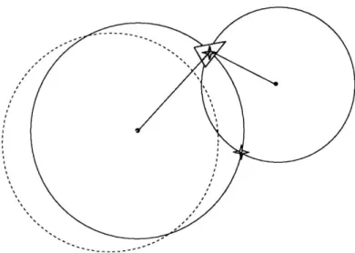
These methods are similar in that they both measure range to the transponders, which requires the vehicle to have an accurate travel time for the interrogation of the transponder and the transponder response. This travel time forms a sphere around the beacon, on which the vehicle lies [13, 22]. Further, the 'BaseLine' to which both of these methods refer is the line of transponders whose position is known. The principal difference between LBL and USBL is that in LBL, the vehicle measures only range to the transponders. Conversely, in USBL, the vehicle measures both range and bearing to the transponder.

LBL navigation

For LBL navigation, the travel times from two or more beacons are used to create spheres on which the vehicle lies. The depth is then measured, turning these spheres into circles at a constant depth, on which the vehicle is located. By using two transponders, two range circles are created which intersect, narrowing the possible vehicle position to one of two intersection points. If a third beacon

Figure 2-1: The travel times from the acoustic returns create range circles around each beacon. The intersection of these range circles provide the vehicle location.

is then added, or if the vehicle knows which side of the 'baseline' it's on, a fix can be obtained as the intersection point of the circles. The case of the two-beacon fix is shown in Figure 2-1. With a calibrated prepositioned transponder grid, accuracies of 1 to 2 meters are possible when acoustic propagation velocity is known [3].

The 'long' term in LBL refers to distance between the transponders, usually on the order of several kilometers.

e USBL navigation

For USBL navigation, the travel time of the signal creates a sphere on which the vehicle lies. This range is combined with a heading, or direction of acoustic return. By measuring depth, the vehicle can now obtain a fix from just one buoy, combining the bearing, range, and measured depth. Accuracy for USBL is expressed as a percent of range between acoustic source and receiver, and typical accuracy is about 1% to 2% of range [3].

The 'ultra-short' term in USBL refers to the distance between receiving hy-drophone elements on the vehicle, which is on the order of centimeters. This small distance allows the vehicle to measure differences in phase of the arriving

2.2.2

Global Positioning System (GPS)

The Global Positioning System (GPS) method utilizes satellites circling the globe for precise position measurements. The system is based upon availability of multiple satellites passing within line of sight view from any point on the earth's surface. Each satellite transmits a unique signal, which includes precise time information along with its 3-dimensional position data [3]. A GPS receiver, after receiving signals from four or more satellites, can compute its 3-dimensional geodetic coordinates.

GPS on its own is accurate only to the order of several to tens of meters. This is

due to ionospheric propagation and U.S. Defense Department introduced "selective availability" errors (to avoid delivering targeting-grade information to other nations). Most, if not all, of these errors can be removed with the use of Differential GPS

(DGPS). A DGPS receiver collects both direct GPS satellite transmissions and signals

from nearby fixed stations that provide error correction information, which are then used to greatly improve the accuracy of a position fix. Accuracies of less than a meter are attainable with the use of DGPS [3, 12].

GPS is very widely used for all applications where the electromagnetic signals

can be detected, which is virtually all navigation requirements. These applications include air travel, sea shipping, and overland commerce. The only requirement for its use is the ability to detect the radio signals emitted from the GPS satellites. It is infeasible for AUV use, however, due to the attenuation of the electromagnetic signal through water. An AUV would have to surface to obtain a GPS fix, which is not desirable or possible in many missions that require great depth or covert operations. The Florida Atlantic University Ocean Explorer AUV and Webb Technologies

SLOCUM glider use dead reckoning, and surface intermittently to get a GPS fix to

bound the error growth. Surfacing for a GPS fix is not possible for deep missions, where travel time from depth to the surface is prohibitive. Further, many mission profiles do not allow the AUV to surface, due to covert operations or vehicle traffic at the surface.

2.2.3

Doppler Velocity Sonar (DVS)

Doppler Velocity Sonar has been used with great success to obtain accurate measure-ments of speed over ground. In this method, several offset down-looking sonars are used to track the bottom of the ocean. By measuring the Dopper shift of the return of each beam, the speed of the vehicle over ground is obtained, both in the along-ship and across-ship directions. [33, 27].

DVS requires space and power on the vehicle, but not more than other sonars. By

providing velocity measurements that are accurate to about 0.2%, the gains obtained in accurate earth-referenced velocity outweigh the space and energy considerations

[6].

2.3

Summary

This chapter has reviewed previous research in navigation for vehicles. We have identified several methods of navigation that are used widely today. Our focus will be in LBL, due to the advantages of sound propagation in water, range, and the ground truth information of an environment measurement. We now proceed to discuss the

Chapter 3

LBL for REMUS operation

The previous chapter has reviewed previous research in navigation for vehicles and drawn us to look closely at LBL as a useful navigation method for AUVs. We begin this chapter by discussing the hardware for REMUS (Remote Environmental Mea-suring UnitS), then describing the LBL method created by WHOI called Sequential LOng Baseline NAVigation, or SLOBNAV.

3.1

REMUS hardware description

REMUS is a small, low cost AUV designed by the Ocean Systems Laboratory at

Woods Hole Oceanographic Institution (WHOI OSL) [32]. A shallow-water vehicle rated to 150 meters, its primary mission is coastal survey and docking with seafloor observatories [1, 9]. In its basic configuration, the 135 cm (53 inch) long, 19 cm (7.5) inch diameter vehicle weighs 31 kg (68 pounds) in air, and is easily handled by a crew of two from a small boat as seen in Figure 3-1.

The standard REMUS survey configuration displacing 40 kg includes 1.2 MHz RD Instruments acoustic Dopper current profiler (ADCP), 600kHz Marine Sonics side scan sonar, conductivity, temperature, and depth recorder (CTD), and optical backscatter sensor (OBS). With the use of Lithium-ion batteries, the vehicle en-durance is 15 hours at 3 knots, covering 80 km. The survey data collected is recorded on the onboard computer system which is based on the PC-104 architecture. Once

Figure 3-1: Vehicle launch from small boat. Photo courtesy of WHOI OSL.

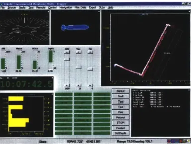
-Figure 3-2: Windows based Graphical User Interface for the REMUS vehicle. This program allows programming missions and downloading mission data when the vehicle is connected

to a laptop or modem. Photo courtesy of WHOI OSL.

docked or connected to a computer on land, data is retrieved and the vehicle pro-grammed via a graphical user interface which runs under Microsoft Windows. The

REMUS interface is seen in Figure 3-2. Note the mission profile in the upper right

corner of the screen, which allows the user to visually check the mission profile.

3.2

REMUS navigation

-

SLOBNAV

REMUS is equipped with an acoustic navigation systems that employs a dedicated

PC-104 based DSP, enabling it to conduct long and ultra-short baseline naviga-tion [28]. In addinaviga-tion, vehicles equipped with an ADCP are capable of bottom lock Dopper navigation. Often all three techniques are used within the same mission. The data from these sensor systems is combined in a position fixing technique that is currently implemented onboard the REMUS vehicle.

REMUS has both a transducer below the nose and hydrophone array on the nose

of the vehicle for transmitting/receiving acoustic signals, as seen in Figure 3-3 and Figure 3-4. The vehicle transducer is used to transmit interrogation pulses to the pre-positioned transponders buoys. The transponder buoy reply is received by the transducer in the LBL configuration, and by the nose array hydrophone in the USBL configuration.

Figure 3-3: REMUS vehicles on bench. Note USBL hydrophone on vehicle nose, and LBL transducer under vehicle nose. Also visible are the four arrays for the ADCP, in the green section of the hull. Photo courtesy of WHOI OSL.

Figure 3-4: REMUS USBL hydrophone with 4 receive elements on vehicle nose, and LBL transducer under vehicle nose. Photo courtesy of WHOI OSL.

Figure 3-5: Sequential long baseline navigation entails moving a transponder location to a new dead reckoned position to obtain a fix with old acoustic data. In this figure, Buoy 1 is dead reckoned to an updated position to obtain a fix with acoustic information from Buoy 2.

For USBL, the nose array has four elements spaced at the four 'corners' of the nose, allowing the receipt time to vary at each element depending on the angle of the incoming signal front, as seen in Figure 3-4. This time delay, or angle of the wave front to the vehicle, gives an angle to the transponder as well as a travel time or range. This range and angle allows the vehicle to compute position from one signal return, making each interrogation cycle a complete navigation cycle.

The LBL cycle, conversely, requires that two separate transponders respond to interrogation cycles for a position fix. To save weight and limit power consumption, REMUS has only one tuned receiver board for incoming transponder signals. It interrogates one transponder at a time, and therefore only receives one range circle each interrogation cycle (see Figure 3-5). To obtain a fix, REMUS will dead reckon the last range circle from transponder A forward to the point where it receives a new range circle from transponder B. As seen in Figure 3-5, this 'sequential' interrogation and dead reckoning of old range information to the new range circle allows REMUS to obtain a fix without simultaneous receipt of transponder ranges, which is typical of an LBL net utilizing more than one receiver board on the vehicle.

Spurious ranges, and consequently spurious fixes, are a common problem for LBL navigation systens. Acoustic multipath, incorrect signal arrival time, and processing

errors lead to misidentifying the first arrival of an acoustic return. This fact requires a vehicle to reject spurious measurements or fixes.

REMUS handles the problem of spurious measurements in several ways [11]. At

the start of each ping cycle, REMUS determines a range gate for the transponder it is interrogating. This determines the sampling window for the data acquisition cycle. Signals outside this minimum and maximum range aren't even acquired for processing. After acquisition, the signal must pass multiple signal to noise tests that enable REMUS to reject (for example) different transponders responding with different codes on the same frequency. Once these SNR tests are passed, the system attempts to compute a lat/lon fix based on the range information obtained. However, the result can be rejected if the new position is outside of an error circle surrounding the vehicles estimated position. This estimate grows linearly with time, and is set by the REMUS navigation programmer.

Using the REMUS onboard navigation algorithm, positioning accuracies of a few meters have been achieved in Navy sponsored tests. In November 1998, REMUS completed a star pattern around a target to study the ability of the sidescan sonar to relocate the target and navigate consistently about the target. The vehicle navigation accuracy was less than 3.5m in a challenging shallow water environment, where water depth was less than 10m [28].

3.3

Summary

In this section we summarized the REMUS hardware and navigation. We discussed the design mission, the sensors employed, and navigation methods utilized by

RE-MUS. This discussion of the navigation will be continued in the next chapter, with

Chapter 4

Extended Kalman Filter for

REMUS Navigation

Having described Long BaseLine navigation, REMUS hardware and REMUS navi-gation (SLOBNAV), we now proceed to discuss the Extended Kalman Filter (EKF). We first consider the general EKF. Then, we examine post-processed REMUS mission data, describing outliers, gating, divergence, and extended acoustic dropout cases. Fi-nally, we discuss the behavior of the on-line EKF.

4.1

Extended Kalman Filter description

The Extended Kalman Filter (EKF) is an optimal recursive data processing algorithm

[5, 21]. Its primary benefit is that all new information, regardless of quality, is

incor-porated to estimate the vehicle state, and therefore position. This is accomplished

by weighting the belief of each new measurement, and adding this information to

update the state accordingly. The outline of the Kalman Filter (KF) and Extended Kalman Filter (EKF) are seen in Figure 4-1 and Figure 4-2. The reader is referred to Vaganay [31] and other references on Kalman filtering such as Bar-Shalom [5] and Maybeck [21] for more background on the EKF.

volution (d the system (true state) Known "nput (control or sensor motin) Estimation of the state

State at tk Input at t State estimate at t

[

Xk) us(k) i(kk)

(k) Tfansition to tk+I State preiction

-- - z(k + 1) = F(t)z(k) t(k + Ilk)

I

+ G(k)ik) + v(k) F(k)i(klk) + G(k)u(k)

Measmrfrnent prediction ;(k+ Ilk) =

H(k + 1).f(k + Ilk)

Measurement at tk+I Measurement rnsdual i(k+i)= v(k+1)=

H(k +1)z(k + 1)+ w(k +1) a(k +1) - i(k + Ilk)

Updated state estimate

i(k +1lk +1)= f(k +1lk)+ W(k+ 1)i(k + 1) state covariance computation State covariance at Ik P(klk)

State ped ction coraiace P(k + Ilk)= F(k)P(klk)F(k)'+Q(k) Innovation covariance S(k + 1) = H(k + )P(klk)H(k + I)' + R(k) Filter gain W(k +I)= P(k + I k)H(k + 1)S(k+

I)-Updated state covariance P(k + lk + 1) = P(k + IlIk)

- W(k + 1)S(k + 1)W(k + 1)'

Figure 4-1: Flow chart of Kalman Filter algorithm. Courtesy of Y.Bar Shalom [5] I

Evolution Known input

of the system (control or Estimation State covariance

( state) sens of the state computation Motion)

State at 4 Input S4 state estkimate at 4t State covaiMance at th

X(k) u(k) k(klk) P(kik)

Evaluation of Jacobians

F(k) = fL

H(k)- 81(k +1)

Transition to (f4 State prediction State prediction covariance

z(k + 1) = --- + *(k + ilk)= P(k +1ik) =

Ilk, z(k).u(k)] + v(k) IPk,&(kk),=(h)) F(k)P(klk)F(k)' + Q(k)

MeOurMMent

(k + Ilk) = I S(k + 1) =

k1k + 1, (k + Ilk)) H(k + 1)P(klk)H(k + 1) + R(k)

M

+ 1) Measurement at Menvremlent ns residual Filter gain

- - s(k +1) = ---- o w(k+1)= W(k +1)=

h'k+J,z(k+1)]+ Uk+1) 4(k+1)-i(k+1Ik) P(k +lIk)H(k+ YS(k+1)-'

Updated state estimate Updated state covariance

k(k+ Ilk + 1) = I P(k +Ilk+ 1)= P(k +Ilk)

k(k+ ilk) + W(k + 1)v(k + 1) - W(k + 1)S(k + 1)W(k + 1)'

Figure 4-2: Flow chart of Extended Kalman Filter algorithm. Courtesy of Y.Bar Shalom

The state vector, x(k), is x(k) = x y 9 U (4.1)

Here, x and y denote position, 0 is vehicle heading, and u is the vehicle velocity. The state transition function fO is given by

x(k + 1) =

x(k + 1)

y(k + 1)

(k +1) u(k + 1)

where A/(k) and Au(k) are known control inputs. The plant model Jacobian F(k) is

F(k)

af(k)

The measurement vector z(k) may vary in length depending on which informa-tion is available at each EKF cycle. Measurements of the vehicle heading, <(k), are provided by a compass, and measurements of the vehicle's forward speed, U(k) are provided by a Doppler velocity sonar. These quantities are updated at a rate of 1 Hz. Range measurements, however, are provided from the REMUS sequential long base-line mode system at a rate of approximately .2 to .5 Hz. The measurement vector, therefore, varies in length for each update of the filter, depending on which measure-ments are available when the EKF is updated. During time steps when Doppler and

x(k) + u(k) cos(9(k))6(t) y(k) + u(k) sin(9(k))6(t)

9(k)+ AO(k)

L

heading information are provided, the measurement vector is:

z(k)= q(k)

U(k)

(4.4)

while during time steps when range measurements to one of the two transponders are provided, the measurement vector is:

z(k) = [ri(k)]

or

z(k) _{= r}

2(k)]

as appropriate. The distances to the transponders, ri(k) and r2(k), are simply:

ri(k) = (xi - x(k))2 _{+ (yi - y(k))2}

r2(k) = V(x2 - x(k))

2_{+ (y2- y(k))2}

where (x1, yi) is the location of transponder 1 and (x2, Y2) is the location of

transpon-der 2.

For heading and speed measurement updates, the measurement model Jacobian

H(k + 1) is H(k + 1) =

Oh(k

Table 4.1: Kalman Filter parameters.

vehicle position process noise standard deviation 0.5 m

vehicle heading process noise standard deviation 0.2 deg

vehicle speed process noise standard deviation 0.05 m/sec

heading measurement noise standard deviation 2.0 deg speed measurement noise standard deviation 0.05 m/sec

range measurement standard deviation 3 m

For beacon 1 updates,

H(k + 1) -Oh(k + 1) _

[

ax x=x(k+1|k)

[(X1-x(k))

(4.10)

For beacon 2 updates,

H(k + 1) aOh(k + 1) =

-

Hxx=*(k+11k)

[

For our post-processed missions, the parameters for the Kalman Filter are listed in Table 4.1. These parameters are determined by operational capabilities of the sensors and our knowledge gained from previous vehicle missions.

The vehicle position process noise standard deviation is due to currents, which add noise to the x and y positions. Based on testing, this is estimated to be 0.5 m. The vehicle heading and speed process noise standard deviations are assumed to be 0.2 deg and 0.05 m/sec, based on testing and assumed current effects.

The measurement noise standard deviation is set by the sensor accuracies. The heading measurement noise standard deviation is listed by the manufacturer to be 1.0 deg; we use a value of 2.0 deg to account for mounting errors and our knowledge of past vehicle navigation results. The speed measurement noise standard deviation is

0.05 m/sec due to the ADCP manufacturer specifications. Finally, the range

measure-ment standard deviation is set to 3 m, based on empirical testing, the use of 12kHz transponders, and the 1000 m to 6000 m operating distances from the transponders. The EKF is initialized with a REMUS SLOBNAV fix during post-processing. This

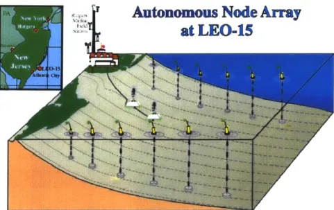
Autonomous Node Array

at LEO-15

Figure 4-3: LEO-15 site as seen from the ocean bottom. The North line buoys are labeled

N1-N6 from the shore, while the South line buoys are labeled A1-A6 from the shore, as

shown in Figure 4-4. Each of the surface buoys and thermistor strings have a transponder positioned 5 meters from the surface for REMUS navigation. Note the permanent nodes in

white, hard-wired to the field station. Photo courtesy of Rutgers University.

initialization assumes the REMUS fix is accurate within several meters. For the on-line mission, filter initialization is assumed to occur with a GPS fix, or by deploying the vehicle at a GPS verified transponder location.

4.2

_{Post-processed navigation missions}

_-

_LEO-15,

July 1999

Data from missions at the Longterm Ecosystem Observatory at a 15m depth (LEO-15) site in New Jersey was collected in July 1999. The LEO-15 site is seen in Figure 4-3. The purpose of the LEO-15 initiative is to provide real-time, 24-hour presence in the ocean for data collection. The location in southern New Jersey was selected due to periodic up-welling events that occur there. Up-welling is a phenomenon where the warm surface waters are driven offshore and cold water is pulled from the ocean bottom to take its place. By taking constant oceanographic measurements, ocean forecasting, much like weather forecasting, can be done to predict future up-welling and physical events offshore. To continuously collect data, two nodes have been

-MO74.4W 74.2W 74.OW

Figure 4-4: LEO-15 buoy lines showing location of line N1-N6 and A1-A6. The North line

buoys are labeled N1-N6 from the shore, while the South line buoys are labeled A1-A6 from

the shore. The REMUS missions used these transponders for LBL missions parallel to the 20 km buoy lines. The location of permanently fixed Nodes A and B, and the Field Station,

are also provided. Photo courtesy of Rutgers University.

permanently mounted on the seafloor, measuring water temperature, salinity, clarity, wave height and period, chlorophyll content, and current speed and direction. The data from these nodes is augmented both with measurements from dedicated research vessels providing radiometers, CTD towed vehicles, and optical profilers, and satellites providing sea surface temperature, water quality and phytoplankton content [26].

There is an increase in up-welling episodes in the month of July. To examine this phenomenon, thermistor strings are added to the LEO-15 site. Comprised of several thermistors mounted on a line extending from the seafloor to a communication buoy on the surface, thermistor strings provide continual temperature recordings from set heights in the water column. This information produces detailed maps of the thermoclines in the area. As seen in Figure 4-3, these buoys are spaced 4km apart in a line from the shore.

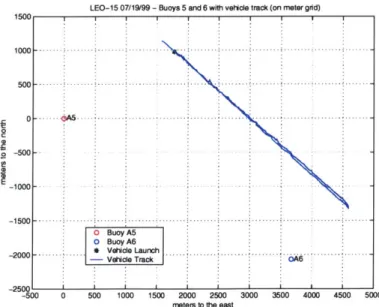
The REMUS missions augmented this data collection in July 1998 by providing a mobile asset to map the water properties along the buoy lines shown in Figure

4-LEO-15 07/19/99 -Buoys 5 and 6 with veticle track (on meter gid) 1500 10 0 0 -. -. .. . -. -. .. -. . -. .. .-.-.-.-.- .. . . . . -. 5 0 0 -. .. .- .. .. - -. .. ... -. . .. . -. .. -. -..-.-.- . .. -.-.-.. .. . * - -500---1000 -- - - ---1500 ... .... - -- - - -- - -- - - - -0 Buoy A5 0 Buoy A6 -2000 .. .. . Ve... Lau nc. . .. .. . .. . . ... . .. ... . .. . .. .

-Vehicle Trackc 0A6

-2500.

-500 0 500 1000 1500 2000 2500 3000 3500 4000 4500 5000 meters to the east

Figure 4-5: Vehicle trajectory for an 80 minute portion of an 8 hour REMUS LEO-15 mission, as plotted by the EKF. A5 and A6 designate the beacon locations. The first 7 minutes of this mission segment are analyzed in more detail in Figure 7 through Figure 4-20.

4. The vehicle's task was to run 20km legs perpendicular to the beach, collecting Conductivity, Temperature, and Depth (CTD) information. These missions often exceeded 15 hours and 70km of continuous data collection.

As described in Chapter 3, REMUS navigates via LBL using two transponders at a time [28]. That is, in the first leg, buoys 1 and 2 are used; the second leg, buoys 2 and 3 are used, and so forth until the vehicle turns around at buoy 6, then the process is reversed. For post-processing, we examined a mission that was performed on July

19, 1999. The portion of the mission we looked at was at the end of the outbound

leg, from Buoy 5 to Buoy 6, and the start of the inbound leg, from Buoy 6 to Buoy

5. This track is seen in Figure 4-5, and is indicative of the whole mission track. As

shown in this Figure, the vehicle runs from Buoy 5 to Buoy 6, turns around, and repeats this track in the opposite direction, heading in toward shore.

4.2.1

Outliers

Any LBL mission will have outliers - range measurements that are incorrect. These are due to multipath, incorrect identification of the first acoustic arrival time, vehicle noise, or processing errors. If these outliers are taken as true range measurements,

the result will be a very 'jumpy' vehicle track, where the vehicle searches for the correct path through the water, chasing outliers. This searching track is undesirable due to the increased power consumption associated with the constant maneuvering. The searching track also does not allow the vehicle to follow a straight-line, yielding poor side-scan data or holidays in the vehicle coverage.

Figure 4-6 shows the ranges from buoys 5 and 6 for a 80 minute portion of the mission. We can see relatively steady returns, and our eyes can intuitively choose which range values are correct. We also see periods of outlier receipt, which are suspect. In this thesis, we examine two parts of this mission portion, then the mission as a whole. First, we focus on a 7 minute portion at the beginning of the interval

(0 to 450 seconds) to study outliers and spurious measurements. Second, the section

from 4400 to 5400 seconds is post-processed to examine extended acoustic dropouts. Period 0-450 will be discussed below, while period 4400-5400 will be discussed in section 4.2.4. Finally, the entire mission is examined in overview.

The key in Figure 4-6 and Figure 4-7 shows three separate measurements: rangeraw, rangeunique, and rangeremus. These three categories are the result of REMUS

SLOB-NAV methods and the need to classify the data as 1) new, unique ranges, 2) ranges

passed from a previous timestep, or 3) ranges accepted by REMUS as 'reasonable', or believable measurements. First, rangeraw refers to all the measurements REMUS logs, which includes all new, passed, and REMUS accepted ranges. REMUS accepted ranges mean those that have passed SLOBNAV tests for reasonable and believable range measurements. Secondly, rangeunique includes all the new measurements (not passed from previous steps), before any tests to deem whether they are acceptable for use. Thirdly, rangeremus is the most exclusive range group, and includes measure-ments that are new ranges which REMUS has deemed acceptable by its measurement acceptance method, described in section 3.2.

To get a better view of the outliers from the 0-450 second period, Figure 4-7 shows the first 7 minutes of the mission between buoys 5 and 6. Differences of 100m are

seen, which represents a 1.5% error in travel time of the acoustic signal.

0

LEO-15 07/19/99 - ranges vs. time

0 1000 20 3000 40 5 6000

Ume (sec)

Figure 4-6: Range returns from buoys 5 and 6 for a 80 minute portion of mission. Note outlier acoustic returns 'jumping' off line of expected returns. A5 and A6 designate the beacon locations. 3800 3600 2400 3200 -? 3000 2800

LEO-15 07/19/99 - ranges vs. time for start of mission

- - A6 rangermw A5 rangeraw + A6 rangeunique a A5 rangetuque o 0 A6 rangerernus 0 A5 rangeremus 0 50 100 150 200 250 300 350 400 450 irne (Sec)

Figure 4-7: Range returns for 7 minute portion of mission. Note outliers of up to 100m from expected return.

-... -. -... -. . . . . . . A 6 range -A range + A6 rangsunique x A5 rangeunique

o A6 rangeremus ... .a... . ..... A... A rangerem us --

.--soon

4000

3000

2000

LEO-i5 07/19- - ranges vs mieafremea rnitsson LEO-I5 071fW99 -LL Ka niwi r ging (cygt ( 501) -KF Eoi dStat

i t Yj yhrt the ib sy

3W O 95 ... . ... ... ... ... + REMUS Fiees 9s sa Vehicle Latngh

340 ks at the.. .. x .es .. ting ... ... t. .. .. s T900

return time (or ~~~liexec)e ag ftetasodr.I h esrmn sdee

igaure,8 Lt, sinadg a the nex measurement for nbsavigaio Tis ewthot gating)

Rigter Yiels ao jumye a t athaorthoe believe s tornyo gte aoirturns. ereodd

Twopateorieso outlier rejection repossbe: imue d omin gaing and tspnata domain tingtrmn [31] The dfferen ccae btwen the hdsistaetw tmemane gaig loosda neacnvda range measurement epasssd Ti arieshad eisatl doainatying

lookt thensfidx reutin from morae thnoe masurement. These methsuaet more a rTe, tme dominethodextmidesd rech wmtasuet upongreiptrmand deterd

returmnie uoratexrae measurement

i u rae a it irems disarded a td he nett measuemnt is.observed. e.Thid, .jmd

as-fornabhe imeaeutse figthe 4-easuresenhisocasd.teltheeEsFrandtseavehaclepttdtas

as is n thr e w f

Spatial~~~~~~~~~~~.. domai out.ier reeto .ehnqe.opt.apsto.ixadte t

frmneacurtrne measurement.(m

Ifo meurens arocepefitota outlier rejection ar osbeiedmeitd, an uptques

Tioabe trakmesults.n Fieto 4-8ashows tah casAlaurement a reit ac etera mieswhthrtht eauemntisacuat bsd n omaisn it hee41ce