Lire
la première p a rtie
de la thèse
Model for prediction of ignition probability
Contents
8.1 Ignition probability models: literature review . . . 132
8.1.1 Pointwise flow characteristics models . . . 132
8.1.2 Trajectory based models . . . 134
8.1.3 Conclusions . . . 137
8.2 Derivation of the model . . . 137
8.2.1 Overview of the model . . . 137
8.2.2 Prediction of the kernel probability of presence . . . 138
8.2.3 Statistical indicators for kernel quenching . . . 147
8.2.4 Combination of both statistics . . . 153
8.3 Results . . . 155
8.3.1 Premixed case . . . 156
8.3.2 Non-premixed case . . . 158
8.4 Conclusions . . . 159 As demonstrated in the previous chapter, LES is able to predict quantitatively the ignition probability. However, the computational cost remains expensive and faster practical tools have been developed for the optimization of combustion chamber. Such methods have been developed in order to predict the ignition probability from the non-reacting flow properties and the empirical knowledge of the ignition process observed from both experiments and numerical simulations.
The objective here is to develop a new model capable of easily estimating the ignition probability based on non-reacting LES flow taking into account the kernel displacement during the early stages of its development. The late flame propagation and stabilization to the injector nozzle are not targeted by the model.
At first, a review of the various methods found in the literature is presented and their limita- tions are highlighted. Secondly, the derivation of the new model is detailed and validated when
131
possible against numerical data extracted from LES. Finally, the results obtained on the KIAI single injector burner in both premixed and non-premixed modes are presented.
8.1 Ignition probability models: literature review
The various ignition probability models presented in the literature can be split in two classes:
models based on local properties of the non-reacting flow and models tracking the spatio-temporal evolution of the kernel. From the literature review presented in Chap.5, one can relate the first class of models to the prediction of kernel generationPkerwhile the second focuses on the whole ignition probabilityPign.
8.1.1 Pointwise flow characteristics models
The first attempt to correlate the ignition probability to non-reacting flow properties has been performed byBirchet al.(1977),Birchet al.(1981) andSmithet al.(1986) in the case of a free methane jet. As mentioned previously (see Sec.5.1.2), these studies demonstrated the correlation between the flammability factor Ff and the probability of successfully creating a flame kernel Pker.Ff is defined as the local probability of finding a flammable mixture at a given location:
Ff = Z zrich
zlean
P(z)dz (8.1)
whereP(z)is the PDF of mixture fractionzandzleanandzrichare the lower and upper flamma- bility limits, respectively. The simplicity of the free jet case allowed to go further andSmithet al.
(1986) constructed a composite formula in order to evaluateP(z) from the first two statistical moments of the measurements. The formula ofP(z)is based on the work ofBilgeret al.(1976) andKent & Bilger(1977) where experiments showed thatP(z)can be constructed from a Dirac delta function and a Gaussian distribution such as:
P(z)c= (1−γ)δ(z−z) +γ 1
√2π z′ exp−(z
−z)2
2z′2 (8.2)
where z and z′ are the mean and RMS values of mixture fraction respectively, δ(x) the Dirac delta function and γ the intermittency factor. Using Eq. (8.1) and Eq. (8.2), the flammability factor is evaluated by:
Ff,c=γ1 2
erf
zrich−z
√2z′
−erf
zlean−z
√2z′
+ (1−γ)δz (8.3)
with δz =
1 ifzlean < z < zrich
0 otherwise (8.4)
This work was recently continued bySchefer et al. (2011) for both methane and hydrogen free jets and the results also showed a good agreement of the reconstructedFf,cwithPker. The range
of position along the jet centerline where overall ignition is possible was found to narrow as the jet velocity is increased.
Although these experiments have brought fundamental understanding of the relation between non-reacting flow quantities and ignition probability, they are restricted to simple configurations with limited practical interest for realistic gas turbine ignition. Recently,Eyssartieret al.(2013) developed a methodology called I-CRIT-LES to predict ignition probability in complex config- urations. Compared to the study mentioned above, this method encompasses the effect of the spark deposit properties, the possible presence of fuel droplets, quenching near walls and the mean velocity at the sparking location. The ignition is successful if the energy deposit validates a series of criteria defined as:
• C1: local mixture equivalence ratio in the flammability range
• C2: power input is sufficient to initiate the chemical reactions
• C3: in two-phase flow, the balance between fuel chemical consumption and evaporation must be in favor of evaporation
• C4: the kernel is not quenched at the walls
• C5: upstream flame propagation is possible
These criteria are evaluated from the combination of several independent snapshots (typically 50 to 100), enabling to construct an ignition probability at each LES grid point and identify the limiting parameter. The model was applied to the two-phase flow MERCATO academic test bench and showed a fairly good agreement with experimental results. The limitation induced by the local formulation of the ignition probability were also highlighted and the model failed in regions where convective effects were dominant.
A similar approach has been developed at ONERA by Linassier (2012) specifically for two- phase flows, with three criteria:
• Criterion 1: ignition of the droplet mist
• Criterion 2: laminar growth of the kernel
• Criterion 3: upstream flame propagation
Once again, the objective is to use local quantities extracted from RANS or LES simulations. The laminar growth of the kernel was computed with the 1D spherical model developed byGarcia- Rosa et al. (2011). The model was also applied to the MERCATO bench and the results are coherent with experiments. As compared to the results of Eyssartier et al. (2013), this model was able to predict the ignition failure in the central recirculation zone due to a more stringent criterion on the droplet mist ignition and kernel growth.
These models based on local quantities extracted from experiments or RANS/LES simulations have been proven relevant to predictPker even though events such as described in the previous
section, where the kernel is convected from non flammable toward flammable mixture, are not captured. However, these models proved deficient by themselves to predict the subsequent flame propagation and overall ignition probability. This motivated the development of models able to take into account the history of the kernel.
8.1.2 Trajectory based models
The first attempt to evaluate the ignitability of a combustor from the non-reacting flow by tracking of the flame kernel was reported in Wilson et al. (1999) where the authors proposed a post-processing technique of RANS solutions. The local value of the Karlovitz stretch factor (Abdel-Gayed & Bradley,1989) was evaluated on the CFD solution and the kernel trajectory was followed by a conserved scalar method. The temporal evolution of the kernel’s fraction experi- encing Karlovitz below the quenching limits ofAbdel-Gayedet al.(1987) was computed and used to estimate the ignition performance. This simple approach was found to reproduce qualitatively the effect of the igniter position and air mass flow rate on ignition performance, but no further validation was available.
The next attempt was reported in the work of Richardsonet al.(2007) based on RANS sim- ulations in a simpler configuration. Inspired by the ATKIM model (Duclos & Colin, 2001), a Lagrangian particle based flame tracking approach was adopted. The model was developed and validated on the experimental configuration ofAhmed & Mastorakos(2006) and applied to sev- eral academic configurations as well as a more realistic combustor designs.
0
0.0 10.0 20.0 -20.0 -10.0
10 30 40
20 50
10 20 30 40 50 60 70 80
Radial position (r/dj) [-]
Axial position (z/dj) [-]
0.0 10.0 20.0 10 30 40
20 50
Radial position (r/dj) [-]
Axial position (z/dj) [-]
0.0 0.1 0.2 0.3 0.4 0.5 0.6 0.7 0.8 0.9 1.0
a) b)
Figure 8.1:Experimental ignition map ofAhmed & Mastorakos(2006) (a) versus spark effectiveness (b).
Extracted fromRichardsonet al.(2007).
The flame propagation was modeled with either a turbulent premixed combustion or an edge flame correlation depending on the local value of the Edge Flame Index (EFI). The EFI is defined as the product of the probability of finding a rich and a lean mixture fraction at a given location.
Its value is maximum where the probability of finding a lean mixture equates that of finding a rich one for which edge flame propagation is used. As one probability becomes dominant, the EFI goes to zero and a premixed combustion regime is considered. A thermal memory effect is included so
that flame particles are not instantaneously quenched when going through an inflammable region.
The particle turbulent convection is treated with a simplified Langevin model with a stochastic Wiener increment to represent the stochasticity of each velocity realization. The particles velocity is the combination of the stochastic convection velocity and the flame velocity. A flame particle is deemed successful if it enters an upstream propagation region before its temperature falls below a critical value. At the beginning of the computation, numerous flame particles are placed at the ignition location and the proportion of successful particles is called spark effectiveness. This model was able to recover the contours of ignition probability in the methane free jet ofAhmed
& Mastorakos(2006) even though some discrepancies were found, as shown in Fig.8.1.
A similar concept was used by Weckeringet al.(2011) in order to evaluate the probability of upstream flame propagation in a free methane jet in a LES framework. Once again, the model was validated on the methane free jet configuration ofAhmed & Mastorakos(2006). The model uses Lagrangian tracking of individual sparking events, and based on experimental evidence, the pointwise Lagrangian particles are replaced by a 35 mm flame kernel after 10 ms. Based on the intersection between the kernel surface and the region where upstream flame propagation is possible, ignition statistics are constructed with the use of the flammability factor at the sparking location. Although the trends given by this model were found in agreement with experiments, the model results were strongly conditioned by user-defined parameters (such as the upstream flame propagation region definition). Similarly toRichardsonet al.(2007), no quenching mechanisms were included in the model.
The SPINTHIR model proposed by Neophytou et al. (2012) aimed at the prediction of the process of flame expansion and overall flame propagation in the combustion chamber. The model was composed of several steps, some of them being derived from the work of Richardsonet al.
(2007). Starting from a time-averaged CFD solution:
• the computational domain is filled with regular grid cells whose state is either cold or burnt
• ignition is modeled by defining an initial spark volume and the cells within this volume are switched to burnt state and release a flame particle
• flame particles are tracked by a stochastic Langevin model based on the CFD solution statistics and can extinguish on the basis of a Karlovitz number criteria. As a flame particle enters a cold state cell, its state is switched and another particle is emitted.
• the ratio of the burnt volume to the total volume of the regular grid πign is tracked in time and at the end of the simulation compared to a critical valueπign,critthat determines whether the ignition try is a success or a failure.
• the probability is evaluated from multiple computations and repeated at several ignition locations to obtain a probability map.
The model was found to reproduce fairly well the ignition maps of several configurations (bluff- body methane burner ofAhmedet al.(2007a), spray burner ofMarchioneet al.(2009) or coun- terflow configuration ofAhmed et al. (2007b)) even though the estimation ofPignwas found to strongly depend onπign,critand to be sensitive to the regular grid resolution and the number of ignition tries. One issue of the model comes from the construction of the ignition probability: a
Monte-Carlo like method is used and a very large number of individual ignition event must be computed to ensure convergency of the result. This could significantly increase the computational cost of the methodology. Another issue is linked to the prediction of the late flame propagation when the flow field can significantly differ from the non-reacting CFD solution due to flame effects. Nonetheless, the model can be used for a quick and cheap estimation of ignition perfor- mances. The SPINTHIR model was improved inSoworkaet al.(2014) by including stochasticity to the local value of the Karlovitz number and introducing history effects on flame particles: a particle entering an inflammable cell is not instantaneously extinguished but changed tohot gas state from which it can either return toburningstate if flammable mixture is encountered again within the next few instants, or extinguish otherwise. The modified model was applied to a lean burn configuration at high altitude conditions and predicted with moderate accuracy the lean ignition limit obtained experimentally for two different designs.
t = 0 ms t = 10 ms t = 30 ms t = 50 ms
Successful event
Failed event
Figure 8.2: Successful and failed ignition events captured with SPINTHIR on a lean burn combustor.
Extracted fromSoworkaet al.(2014).
Finally,Cordieret al.(2013b) developed a model based on the same philosophy as SPINTHIR to evaluate the ignition performance of the single injector KIAI burner using experimental data.
The model tracks flame particles emitted from the ignition location using a simplified Langevin equation, and the stochasticity of the non-reacting velocity field is included through a random draw of the field in the experimental database. Each particle represents a flame kernel whose growth is computed based on literature correlations and can be divided in two separate particles if its size exceeds the local value of the integral length scale. Quenching of flame particles is incorporated using a critical Karlovitz number criterion. Ignition success is conditioned on both the number of particles and their location at the end of the simulation. The model was able to reproduce some of the main features of the experimental probability map and ignition scenario but locally deviated from experiments in regions of intense turbulence. Since the ignition prob- ability is constructed with the same methodology as the SPINTHIR model, it also suffers from the issue regarding the number of individual ignition events required to ensure the convergence of the Monte-Carlo method.
8.1.3 Conclusions
As demonstrated in this short review, models based solely on local flow characteristics are compu- tationally very cheap and provide insight on the spark performances but appear to be inadequate to capture ignition failure occurring later during the kernel phase. On the other hand, track- ing based models encompass the kernel transport effects but do not focus specifically on kernel quenching and suffer from convergence issue.
In the following, a new model is derived with the objective of taking advantage of both afore- mentioned approaches: the low CPU cost of pointwise model is kept in a new approach combining it to transport effects through an evaluation of a statistics of the kernel trajectories.
8.2 Derivation of the model
The objective is here to develop a model capable of predicting the ignition probability from non- reacting flow statistics. As compared to the previous model I CRIT LES developed at CERFACS (Eyssartieret al.,2013), the aim is to incorporate some of the time history effects. This point cad indeed the main weakness of the I CRIT LES methodology, and its importance was highlighted in the fully resolved LES ignition sequences performed in Chap. 7. Driven by the increasing computational power, the number of elements of the LES meshes used for industrial studies increases leading to a growth of the memory requirements. Thus, to simplify the application of the present model, one constraint is to only use time-averaged CFD fields to estimate the ignition probability.
8.2.1 Overview of the model
The model focuses on the prediction of the ignition probability at the end of the kernel expansion phase, thus evaluating the probability of success ofPhase 1 and of the beginning ofPhase 2.
This choices is motivated the LES results presented in Chap.7where most of the failures occured within the first 5 ms after energy deposit. The kernel quenching was the consequence of two mechanisms: 1) inflammable mixture pockets could locally quench the flame front or even prevent the kernel formation, 2) kernel/turbulence interactions could lead to large scale deformations of the kernel and induce flame/flame interactions and flame front stretching. Thus, to construct the ignition probability, two elements are combined as schemed in Fig.8.3:
• a statistic of the kernel motion is evaluated by constructing the temporal evolution of the kernel presence probability density functionPpres(x, t).
• statistics of the non-reacting flow characteristics are evaluated at each grid point to encom- pass possible quenching of the flame kernel.
Both statistical information are then combined to provide an estimation of the ignition probabil- ity.
Kernel presence probability density
function
Non-reacting flow statistics
Ppres(x, t)
Combine both statistics
Ignition probability
Ka(x) Ff(x)
Figure 8.3: Overview of the model elements.
More precisely, the algorithm of the model is described by the following steps:
• Perform a non-reacting CFD simulation to obtain time-averaged fields (velocity, mixture fraction).
• Compute statistical indicators required to evaluate the local occurrence of quenching, from non-reacting flow statistics
• Use the spark characteristics to evaluate the kernel size and the time required to drop from the high temperature of the kernel to the adiabatic flame temperature. This step is performed in 0D assuming that the kernel temperature is only dictated by the balance between reaction rate and turbulent dissipation.
• Compute the temporal evolution of the kernel, by constructing its probability of presence combined to the indicators of step 2. The kernel growth is also computed, and if the kernel size is beyond a critical value, the kernel is considered to successfully ignite the burner since local quenching can no longer result in global quenching.
8.2.2 Prediction of the kernel probability of presence
In contrast with previous models using Lagrangian tracking of individual kernels (Neophytou et al.,2012;Cordier,2013), the present model intends to track the kernel displacement through its presence PDFPpres(x, t). The main idea is to use the cold flow statistics to reconstruct kernel trajectories statistics, rather than recalculating numerous individual trajectories. At first, the validity of the hypothesis required to construct Ppres(x, t) are evaluated in Sec. 8.2.2.a. Then, details of the construction ofPpres(x, t)are presented in Sec.8.2.2.band the results are partially validated in Sec.8.2.2.c.
8.2.2.a Evaluation of the hypothesis validity
To construct the kernel probability of presence, three hypotheses have been made:
• H1: the velocity components follow a Gaussian distribution.
• H2: the statistics of the non-reacting flow (mean and fluctuations) are not modified during the first milliseconds after energy deposit.
• H3: the self-propagating velocity of the flame is low compared to the total flame velocity (using notation introduced in Sec.3.2.1.b:Sa> Sd)
The validity and limitations of these hypotheses are evaluated using the LES results. H3has already been evaluated in Sec.7.4.2.b where the PDF of flame displacement speedSd has been shown to be much smaller than the absolute flame velocitySa.
H1: Velocity components Gaussian distribution
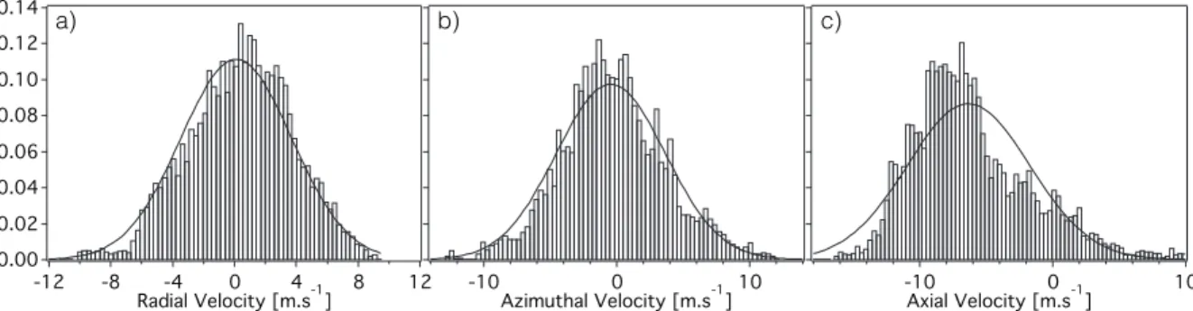
The first assumption necessary to derive a model predicting the kernel presence PDF is that the velocity components follow a Gaussian distribution. Although this assumption is perfectly true from a turbulence point of view (Pope, 2000), it is often made when deriving models. To evaluate the validity of this assumption in the present case, PDF of velocity components are constructed from temporal recording at numerous locations in the computational domain of the LES. The data are recorded during 100mscorresponding to more than 25 rotations of the PVC.
An example of obtained distributions is shown in Fig.8.4along with the corresponding Gaussian distribution.
a) b) c)
0.14 0.12 0.10 0.08 0.06 0.04 0.02 0.00
PDF [-]
-12 -8 -4 0 4 8 12
Radial Velocity [m.s-1] 0.14 0.12 0.10 0.08 0.06 0.04 0.02 0.00
-10 0 10
Azimuthal Velocity [m.s-1] 0.14 0.12 0.10 0.08 0.06 0.04 0.02 0.00
-10 0 10
Axial Velocity [m.s-1]
Figure 8.4: PDF of the three velocity components atz/Dext = 0.5 and x/Dext = 0.0 along with the Gaussian distribution (lines).
For this particular position, the Gaussian assumption seems to be valid for radial and az- imuthal velocity components but the axial component exhibits a significant positive skewness, of factor γ1 = 0.89. This skewness factor, which can be viewed as a measure of the deviation to Gaussian distribution, is mapped from 1326 probes on Fig.8.5.
The results show that, departure from a Gaussian distribution can be locally significant. The radial velocity component exhibits strong positive skewness factor in the CRZ while the axial velocity skewness is significant in the IRZ. However, for the largest part of the map, the skewness factor stays in the [-1,1] range for which a Gaussian approximation is reasonable for the level accuracy desired for the approach.
H2: Kernel effect on the velocity field
Axial velocity skewness Azimuthal velocity skewness
Radial velocity skewness 0.0
-1.0 2.5
0.0
-1.3 0.7
0.0
-1.3 1.9
Figure 8.5: Map of skewness factor γ1 for the three components of velocity in a y-normal cut plane through the center of the combustion chamber.
It is assumed that during the early instants after energy deposit, the statistics of velocity are not greatly modified in the region where the kernel develop and stay those of the cold flow. This assumption is expected to be inadequate at longer times due to the modification of the fresh gases aerodynamics induced by the kernel expansion.
Figure 8.6: Sampling boxes for the construction of spatial distribution of velocity for ignition at PT1.
To estimate the limits of this assumption, three cubic boxes of increasing size centered at the energy deposit location are defined (c= 1.5,2and3cm). An example of these boxes for ignition at PT1 is shown in Fig.8.6. The grid vertices located in these boxes are then used to build the spatial PDF of the velocity components. The small box is sufficient to evaluate the effect of the kernel during the early instants after energy deposit, but kernel growth and displacement might bring the kernel out of the box. On the contrary, the kernel stays within the limits of the larger box during its entire growth, but the large number of sample points masks the changes in the PDF shape. All three boxes are tested here to highlight the effect of the sample size on the PDF evolution in time.
In order to take into account the flow unsteadiness, several instantaneous solution of the non- reacting flow are employed. The PDF is then computed at several instants after energy deposit during the kernel growth. An example of the results is presented in Fig. 8.7 for an ignition sequence at PT1 for thez-axis and the x-axis velocity components (note that in this case, the PDF of thex-axis and the y-axis components are the same). The grey zone corresponds to the inert flow envelope (mean±RMS) and the PDF at four instants are plotted. Prior tot= 2.2ms the PDF lies within the grey region but the PDF gradually shifts as time proceeds.
0.05 0.04 0.03 0.02 0.01 0.00
PDF [-]
-30 -20 -10 0 10 20 30
x-axis velocity [m.s-1] Non-reacting
t = 2.2 ms t = 3.0 ms t = 3.8 ms t = 4.8 ms 0.04
0.03
0.02
0.01
0.00
PDF [-]
40 30 20 10 0 -10 -20
z-axis velocity [m.s-1]
Non-reacting t = 2.2 ms t = 3.0 ms t = 3.8 ms t = 4.8 ms
Figure 8.7:Comparison of axial (left) and radial (right) velocity components PDF between non-reacting (grey area) and ignited cases at several instants after ignition at PT1 using the intermediate 2 cm square box. The full line is the mean non-reacting flow PDF.
The effect of the box size is illustrated in Fig.8.8where the PDF ofz-axis velocity component at PT1 is plotted for the three boxes. For the larger box, the number of nodes is so high that the PDF is barely affected by the kernel growth even after long times. On the other hand, the small box is more erratic, with significant changes of the PDF already att= 2.2msand opposite trend att= 4.8 ms. This results from the fact that the kernel has extended beyond the limits of the sampling box att= 4.8ms.
The time limit at which the modification of the PDF is too important to consider that the non- reacting velocity statistics are still relevant is subjective and changes from one ignition location to the other. A general trend is that past 2 ms, the PDF not anymore representative of the non- reacting flow. Going back to the temporal evolution of the global heat release plotted in Figs.7.9, 7.12&7.15, this critical time of 2 ms appears greater than most of the failed events captured in LES. It can be then assumed that the cold flow statistics can be used.
8.2.2.b Construction ofPpres(x, t)
The time-averaged statistics of the non-reacting flow are obtained from the LES simulation. The meanuiand RMSu′iof thei-th component of velocity are then used to construct the PDF of the
0.06 0.05 0.04 0.03 0.02 0.01 0.00
PDF [-]
40 20
0 -20
z-axis velocity [m.s-1]
Non-reacting t = 2.2 ms t = 3.0 ms t = 3.8 ms t = 4.8 ms
0.04
0.03
0.02
0.01
0.00
PDF [-]
40 20
0 -20
z-axis velocity [m.s-1]
0.08
0.06
0.04
0.02
0.00
PDF [-]
40 20
0 -20
z-axis velocity [m.s-1]
a) b)
c)
Figure 8.8: Effect of the box size on the PDF of velocity. From left to right,c=1.5 (a), 2 (b) and 3 (c) cm. Non-reacting case is represented wit the grey area.
velocity componentui, assuming a Gaussian shape:
P(ui) = 1
√2π u′iexp−
(ui−ui)2 2u′2
i (8.5)
The aim is now to construct the envelope of the possible trajectories, with the mean trajectory given byuiand its dispersion resulting ofu′i. The velocity Gaussian PDF must be transformed in a position PDF. Starting from the definition of the velocity in 1Ddx/dt=u, the PDFs of velocity and position are related by:
dP(x)
dt =P(u) (8.6)
andP(x)can be evaluated by integration ofP(u):
P(x) = Z
P(u)dt=P(u).dt=P(u.dt) (8.7)
whereP(u) is supposed to be independent of time and the time step dt is constant. P(x) can then be rewritten fromP(u):
P(x0, x) = 1
√2π u′i.dtexp−
(x−µ)2 2(u′
i.dt)2 (8.8)
where the argumentx0 is added to indicate the emission point andµis the mean position of the kernel corresponding to the convection by the mean flow:
µ=x0+u.dt (8.9)
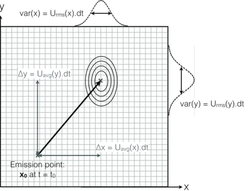
In a multidimensional case, a multivariate Gaussian distribution is used and an example of the kernel presence PDF field is schematically illustrated in Fig.8.9where the probability of finding at timet0+dta particle emitted from a single pointx0at timet0is represented in 2D.
60
40
20
y
x
Emission point:
x0 at t = t0
60
40
20
∆y = Uavg(y).dt
∆x = Uavg(x).dt var(x) = Urms(x).dt
var(y) = Urms(y).dt
Figure 8.9: 2D schematic illustration of the probability of presence field att =t0+dtresulting of the emission of a point atx0att=t0.
When considering the general case of an ensemble of emission points in a three-dimensional case, the kernel presence PDF at point xPpres(x, t) is the sum of all possible trajectories con- tributing to the kernel presence PDF, given by:
Ppres(x, t) = XN n=1
Ppres(xn, t−dt).V((xn)
| {z }
Probability of being at point xnatt−dt
P(xn,x)
| {z }
Gaussian PDF of x for an emission atxn
(8.10)
where N is the number of nodes having a non-zero probability of presence at time t−dt, xn andV(xn)are the coordinates and the nodal volume of then-th node respectively, andP(xn,x) is the multivariate Gaussian distribution giving the PDF value ofxfrom an emission point xn. P(xn,x)is the three-dimensional extension of Eq. (8.8):
P(xn,x) = 1
p(2π)3|Σn|e−12(x−µn)TΣn−1(x−µn) (8.11) where µn and Σn are the mean position and covariance matrix of the multivariate Gaussian distribution of the n-th emission point. The Gaussian distribution is normalized to ensure that R
V Ppres(x, t)dx= 1. The mean position vector components are given by:
µi,n=xi,n+ui,n.dt (8.12)
where ui,n is the time-averaged velocity i-th component at node n. The covariance matrix is obtained from the RMS of the non-reacting flow:
Σn =
(u′x,n.dt)2 0 0 0 (u′y,n.dt)2 0 0 0 (u′z,n.dt)2
(8.13)
whereu′i,nis the i-th velocity component RMS. Note that as a first step only the diagonal terms are kept, but off diagonal terms could be taken into account to encompass correlations between velocity components. The model then entirely relies on the velocity statistics of the non-reacting flow to evaluate the temporal evolution of the probability of presence through the computational domain. The computation is initiated by setting Ppres(x, t) = 1/V(nspark) at the closest grid point from the exact spark positionnspark.
8.2.2.c Application to the KIAI burner anda-priori validation
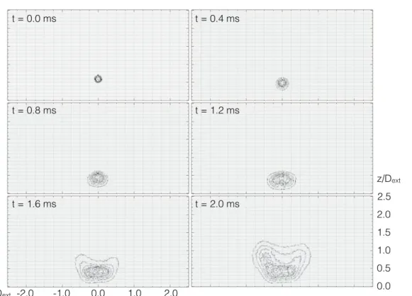
An example of the result is given in Fig. 8.10 as iso-contours of the probability of presence for a spark located atx/Dext = 0.0 and z/Dext = 0.6 and the results are projected in the 2D x-z plane to ease the visualization. At first, the probability of presence is found to follow the motion of the IRZ toward the methane jet with little spreading since the turbulent intensity is low.
As it reaches the stagnation point, the PDF spreads radially toward the SWJ due to the high turbulence intensity and is then rapidly convected downstream by the high axial velocity of the SWJ.
In order to validate at least qualitatively the prediction of the model, the full LES of ignition sequences presented in the previous Chapter are post-treated individually to evaluate the proba- bility of finding a flame element in space at a given instant after energy deposit. The probability of finding a flame element is given by:
Pf l(x, t) =
NXLES
s=1
V(n) PN
n=1V(n) (8.14)
whereNLES is the number LES full ignition sequences used,N is the number of vertices having a heat release rate above1.0e6 W.m−3 andV(n)is the volume associated with then−th node.
t = 0.0 ms t = 0.4 ms
t = 0.8 ms t = 1.2 ms
t = 1.6 ms t = 2.0 ms tt = 2.0 ms tt =t =t =tttttttt = 2.0 ms = 2 = = = = = = = = = = = = 2 2 2 2 2 2 2 2 2 2 2 2 2 2.0.0 m.0 m.0 m.0.0.0.0.0.0.0.0.0.0 ms m m m m m m m m m m m m m m m ms s s s s s s s
0.0 1.0 2.0
-2.0 -1.0 0.0
0.5 1.0 1.5 2.0 2.5 z/Dext
x/Dext
Figure 8.10: Temporal evolution of projected probability of presence iso-contours for an ignition at x/Dext= 0.0andz/Dext= 0.6predicted by the model.
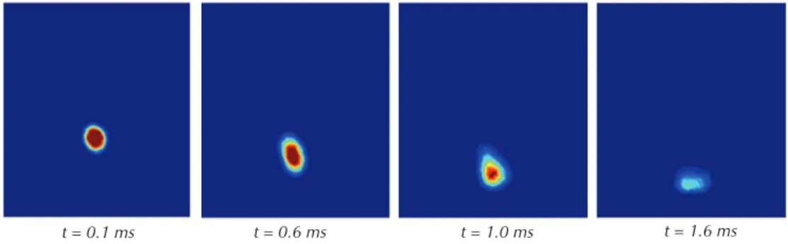
Note that this LES result intrinsically includes the extinction of flame elements due to the local flow characteristics. The number of LES sequences used to evaluatePf l(x, t)is small (maximum 15, depending on the number ignition event failing to initiate a flame kernel), so thatPf l(x, t)is poorly converged, which becomes less representative as time advances. For each ignition location studied with LES, several snapshots of the flame position are presented in Fig.8.11and compared to the model predictions.
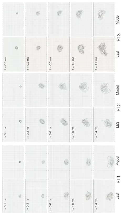
The model is found to reproduce fairly well the trend observed from the ensemble averaged LES results. At PT1, the model probability of presence is first convected downstream before being deflected from the injector axis near the stagnation point. In the LES, the kernel is also convected towards the methane jet at first, but the convection ofPf l(x, t) at longer time is not observed. This difference can be related to the strong occurrence of quenching in the methane jet region observed in LES (see Fig.7.24), not included in the evaluation ofPpres(x, t). At PT2, the model predicts both the convection of the kernel downstream due to the SWJ and the upstream motion induced by the IRZ. In the LES, large chunk of flame in the SWJ are quenched due to the lean mixture composition and since this effect is not taken into account in the model, the probability of presence in the SWJ is significant while rapidly dissipated in the LES. For PT3, the bulk convection of the kernel downstream is well captured by the model even though the small number of LES sequences results in a inward displacement of the probability, stronger than the model prediction. Although this validation of the kernel presence PDF is only qualitative, the model seems to reproduce the main motion of the kernel and the objective is now to use the
PT1LESModelLESModelLESModel PT2PT3
t = 0.1 ms t = 0.1 ms t = 0.1 ms t = 0.3 ms t = 0.3 ms t = 0.3 ms t = 1.4 ms t = 1.4 ms t = 1.4 ms t = 1.0 ms t = 1.0 ms t = 1.0 ms
t = 0.6 ms t = 0.6 ms t = 0.6 ms
Figure 8.11: Comparison ofPpres(x, t)evaluated by the model and Pf l(x, t)computed from the LES database at the three ignition locations studied in Chap.7at 5 instants.
knowledge of the flame position to evaluate the underlying flow properties and the probability of ignition success.
8.2.3 Statistical indicators for kernel quenching
From the analysis of the LES results presented in Chap. 7, the two main flow characteristics affecting the ignition success are the mixture composition and the turbulence intensity. In this section, statistical indicators based on these mechanisms are built.
8.2.3.a Mixture composition Flammability factor
The various ignition studies in non-premixed flow available in the literature clearly point out the fact that the flammability factorFf is a critical parameter (Birchet al.,1977;Ahmed et al., 2007a;Neophytouet al.,2012;Eyssartieret al.,2013). This is also confirmed by the present LES of fully resolved ignition: Ff is closely related to the probability of creating a sustainable flame kernel or leading to quenching. The time-averaged statistics obtained from the non-reacting LES can then be used to construct the flammability factor statistics, similarly to the early work of Birchet al.(1977) andBirchet al.(1981). As mentioned in Sec.8.1.1, these studies proposed to use a composite PDF to evaluate the flammability factor from the measured mixture field average and RMS values. In the free methane jet case, the combination of a Gaussian and a delta Dirac functions provided a fairly good estimate ofFf. In the more complex flow pattern of the KIAI burner, a wide variety of PDF are encountered and simple PDF are less accurate.
A map based on 1326 probes, where the temporal evolution of mixture fraction was recorded, is constructed from the non-reacting LES simulation presented in Chap.6. The map covers the same area as the experimental ignition probability map presented in Fig.7.1and focuses on the vicinity of the methane jet. At each probe, the mixture fraction is recorded during 100 ms at a frequency of 50 kHz in order to obtained converged first and second statistical moments of the mixture fraction distribution and build a PDF of z sufficiently resolved. To investigate further the PDF moments, a map of skewness factorγ1is also constructed and plotted in Fig.8.12.γ1 is given by:
γ1 = z3−3zz′2−z3
z′3 (8.15)
In Fig.8.12, the first two statistical moments are similar to the results showed in Fig.6.9. The magnitude of the skewness factor clearly indicates that the Gaussian hypothesis does not hold in a large part of the combustion chamber. Note that the map exhibits on the top a high skewness but small RMS, indicating that the PDF is narrow. The skewness factor is mainly positive, which means that the most probable value ofzis lower than its mean.
From the recorded PDF of z, the flammability factor can be directly evaluated and will be used as reference. The map of Ff is shown in Fig. 8.13 along with the PDF of z at several locations. The flammability factor is found to go from zero near the methane jet and the swirler
Skewness of mixture fraction RMS of mixture fraction
Mean mixture fraction 0.0
1.0
0.0 0.31
0.0
-2 3
Figure 8.12:From left to right: maps of mean, RMS and skewness factor of the mixture fraction PDF in ay-normal cut plane through the center of the combustion chamber.
inlet, to one in the downstream region where the time allowed for mixing is longer, leading to a mixture fraction near the overall equivalence ratio and with small RMS value. The PDFs ofzat a few selected locations give an overview of the wide variety of mixing behavior resulting from the complex flow pattern. PDF labeled a) was picked in the wake of the wall separating the SWJ and the methane jet, where mixing is controlled by the turbulence and the large helical structure of the PVC: the PDF peaks in pure air but has a strong probability of mixture near stoichiometry and a long tail toward rich mixture. PDF b) is spread from pure air to pure methane, with a peak in pure methane. The nearly equi-probability over a wide range ofzindicates that this location is in the mixing layer between the pure methane of the jet and the lean flow from the IRZ. Located further downstream on the injector axis, PDF c) peaks in rich but flammable mixture indicating that the lean flow from the IRZ has been enriched by diffusion from the pure methane jet. PDF given in d) is located in the shear layer between the SWJ and the IRZ and its most probable value is near stoichiometry, but there is a significant probability of finding pure air due to the PVC structure. PDF e) is in the SWJ, but the pure air is mixed to a certain extent with the fuel so that the probability of finding mixture between 0 and 0.05 is strong but rapidly decreases for higherz. Finally, PDF f) is located in the SWJ but close to the entry plane so that very little mixing has occurred yet and pure air is mostly found.
From the PDF provided in Fig. 8.13, it appears that estimating Ff based presumed PDF parametrized by the mean and RMS values of thez field only, will not be accurate. Following Birchet al.(1977), tests for three PDF shapes are made:
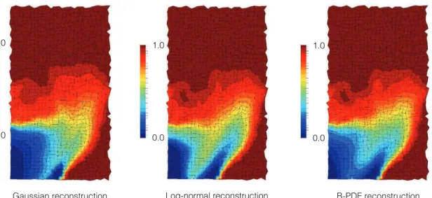
• Gaussian distribution:
Ff,gauss= 1 2
erf
zrich−z
√2z′
−erf
zlean−z
√2z′
(8.16)
Flammability factor 0.0
1.0
6 4 2 0
PDF [-]
1.0 0.8 0.6 0.4 0.2 0.0
Mixture fraction !" [-]
20 15 10 5 0
PDF [-]
0.6 0.4 0.2 0.0
Mixture fraction !" [-]
25 20 15 10 5 0
PDF [-]
0.25 0.20 0.15 0.10 0.05 0.00
Mixture fraction !" [-]
16 12 8 4 0
PDF [-]
0.5 0.4 0.3 0.2 0.1 0.0
Mixture fraction !" [-]
30
20
10
0
PDF [-]
0.8 0.6 0.4 0.2 0.0
Mixture fraction !" [-]
300
200
100
0
PDF [-]
0.05 0.04 0.03 0.02 0.01 0.00
Mixture fraction !" [-]
a) b)
c) d)
e)
f)
Figure 8.13:Map of flammability factorFfobtained from LES recorded PDF(z). From a) to f), PDF of zat a few selected locations in the mixing region.
• Log-normal distribution:
Ff,logN = 1 2
erf
ln(zrich)−µ
√2σ2
−erf
ln(zlean)−µ
√2σ2
(8.17) whereµandσ are the log-normal law parameters given by:
µ= ln(z)−1 2ln
1 + z′
z2
and σ = ln
1 + z′ z2
(8.18)
• β-PDF distribution:
Ff,β =Izrich(α, β)−Izlean(α, β) = Bzrich(α, β)
B(α, β) − Bzlean(α, β)
B(α, β) (8.19)
whereBz(α, β)is the incomplete beta function andIz(α, β)the regularized incomplete beta function of parametersαandβ given by:
α=z
z(1−z) z′ −1
and β= (1−z)
z(1−z) z′ −1
(8.20) Note that theβ-PDF is found to diverge for very high values ofβ, so that Ff,β = Ff,logN wherez′ <1.0e−2.
The reconstructed fields ofFf based on the three presumed PDF shapes, using the moments from the LES, are presented in Fig. 8.14 and compared to the map obtained from the true z- PDF presented in Fig. 8.13. As expected from the good mixing properties of the injector, all reconstructedFfreproduce quite well the downstream region where mixture fluctuations are very