Aid and Income Stabilization

(1)

HAL Id: halshs-00554289

https://halshs.archives-ouvertes.fr/halshs-00554289

Preprint submitted on 10 Jan 2011

HAL is a multi-disciplinary open access archive for the deposit and dissemination of sci-entific research documents, whether they are pub-lished or not. The documents may come from teaching and research institutions in France or abroad, or from public or private research centers.

L’archive ouverte pluridisciplinaire HAL, est destinée au dépôt et à la diffusion de documents scientifiques de niveau recherche, publiés ou non, émanant des établissements d’enseignement et de recherche français ou étrangers, des laboratoires publics ou privés.

Sylviane Guillaumont Jeanneney, Sampawende Jules Tapsoba

To cite this version:

Sylviane Guillaumont Jeanneney, Sampawende Jules Tapsoba. Aid and Income Stabilization. 2011. �halshs-00554289�

(2)

1

Document de travail de la série Etudes et Documents

E 2009.16

Aid and Income Stabilization

S. Guillaumont Jeanneney and S. J-A. Tapsoba1

June 2009

1

Centre d’Etudes et de Recherches sur le Développement International (CERDI), Université d’Auvergne CNRS, 65 boulevard François Mitterrand, 63000 Clermont-Ferrand.

Corresponding author : Sylviane Guillaumont Jeanneney, La Gagère, 63190 Bort l’Etang, France, phone : 33473684083, mail : s.guillaumont@u-clermont1.fr

(3)

2 Abstract

This article contributes to the debate on aid volatility and argues that official assistance copes with exogenous output shocks in recipient countries and stabilizes resources available for the financing of consumption, investment and net trade. Stabilizing aid is effective in aid-dependent and vulnerable states. Aid volatility and disbursement lags are not significant determinants of the stabilizing impact of aid.

Résumé

Cet article participe au débat sur l’instabilité de l’aide au développement et soutient que celle-ci fait face aux chocs exogènes qui affectent la production et stabilise les ressources nationales finançant la consommation, l’investissement et la balance commerciale. Le rôle stabilisateur de l’aide est particulièrement présent dans les pays fortement dépendants de l’aide et dans ceux les plus vulnérables aux chocs extérieurs. Ni l’instabilité de l’aide ni ses délais de déboursements n’apparaissent comme des facteurs déterminants du rôle stabilisateur ou non de l’aide extérieure.

Keywords: Foreign aid, Income stabilization, Developing countries. JEL Codes: F35, E32, E60.

(4)

3 1 Introduction

Official foreign aid is a major source of revenue for developing countries. Its effectiveness in terms of growth and poverty reduction is a much-debated question. No clear consensus has emerged on either theoretical or empirical grounds. Burnside and Dollar (2000) and Collier and Dollar (2002) argue that aid effectiveness depends on sound economic policies and good institutions. In contrast to this main stream, Guillaumont and Chauvet (2001) have shown that a major factor conditioning aid effectiveness in recipient countries is the economic vulnerability they face. This last factor is due to external shocks or climatic events and natural disasters. If economic vulnerability is a determinant of aid effectiveness, it is mainly due to its stabilization impact. Collier and Dehn (2001) have demonstrated the positive effect of increasing aid during negative shocks in relation to the terms of trade. Thereby, aid is an important device to cope with output fluctuations. Corresponding welfare gain might be sizeable2.

The stabilization properties of aid have recently become the cornerstone of the debate. In this new controversy, there is a growing point of view suggesting that aid is an important source of macroeconomic instability as it is volatile and thus unpredictable in many developing countries. Therefore uncertainty in aid flows might undermine its effectiveness (Lensink and Morrissey, 2000 and Hudson and Mosley, 2008)3. As a consequence in the Paris declaration of 2005, donors have committed to improve the predictability of aid disbursements by raising their multi-annual aid commitments. Most notably, aid tends to be procyclical rather than countercyclical, i.e. disbursements increase during expansion episodes and decrease in recession periods. Aid has failed to act either as a stabilizing force or as an insurance mechanism (e.g. Gemmell and McGillivray 1998, Pallage and Robe 2001, Bulir and Hamann

2

Pallage and Robe (2003) estimate that macroeconomic fluctuations are much stronger and costly in developing countries than in the United States. For example, on average, the welfare cost of output volatility in sub-Saharan Africa could be as much as 15-20 times higher than that in the United States. Furthermore, Kose (2002) obtains that most of the shocks in developing countries have exogenous roots.

3

Lensink and Morrissey (2000) were the first to notice that aid uncertainty might be a dimension of aid effectiveness. They estimate in a growth equation that aid volatility reduces aid effectiveness. Hudson and Mosley (2008) confirm that aid volatility has a negative impact on growth. The differentiation between positive and negative volatility indicates that the damage is caused by positive volatility.

(5)

4

2003, 2008, Hudson and Mosley 2008 and Fielding and Mavrotas 2008)4.

However, the link between aid volatility, aid cyclicality and stabilizing aid is not self-evident. Even if aid is procyclical, it can be stabilizing if its fluctuations are lower than those of the output. Countercyclical aid might be destabilizing if aid fluctuations are higher than the output ones. According to the magnitude of its variability, procyclical or countercyclical aid could smooth out exogenous output shocks in recipient countries. In a stabilization purpose, aid flows cannot be expected to be completely stable through time. Thus, analyses based on aid volatility could be misleading, since they overshadow the compensatory property of aid. Compensatory or stabilizing aid is more relevant than aid volatility (e.g. Chauvet and Guillaumont 2009)5.

This article focuses on the compensatory or stabilizing profile of official aid in recipient states experiencing GDP fluctuations. Our paper is connected to the works of Gupta et al. (2004) and Pallage et al. (2006). On the one hand, Gupta et al. (2004) examine cyclical properties of food aid with respect to food availability in recipient countries on a large sample of developing and transition economies. They show that food aid is countercyclical in countries with the greatest need for such aid and insufficient means to mitigate contemporaneous shortfall in consumption. On the other hand, Pallage et al. (2006) show that changing the timing of aid flows could substantially smooth consumption and ease the welfare costs of macroeconomic fluctuations in recipient countries. However, our approach is different. We leave the debate on cyclical aid aside. We are interested in the role of official aid in coping with exogenous fluctuations in Gross Domestic Product (GDP). We assess the contribution of aid in the stabilization of resources available for the financing of consumption, investment and net trade in recipient after an output shock.

We use a method based on national accounts initiated by Asdrubali et al. (1996) in order to identify flows that are able to ensure public or private consumption in industrial countries

4

Gemmell and McGillivray (1998) were the first to comment on aid instability. They show that, with the exception of capital revenues, aid flows are the most volatile. Likewise, Pallage and Robe (2001) and Bulir and Hamann (2003, 2008) obtain that aid is highly volatile, unpredictable and overwhelmingly procyclical. Hudson and Mosley (2008) and Fielding and Mavrotas (2008) estimate that lesser aid instability is associated with good institutions, sound policies, a large number of donors and a high dependency on circumstantial aid, such as food aid, emergency aid, and program/budget support aid.

5

Chauvet and Guillaumont (2009) compare the volatility of exports to the volatility of aid plus exports. They find that aid contributes to the dampening of the volatility of exports of goods and services.

(6)

5

against asymmetric shocks6.

Our results indicate that foreign aid is partly stabilizing and could be used as an insurance device in developing countries. We also find that aid dependency and output volatility increase the effectiveness of stabilizing aid. Further, aid volatility or disbursement lags (i.e. the inverse of disbursement speeds) do not appear as significant determinants of the stabilizing impact of aid. .

The remainder of the paper is structured as follows. Section 2 describes the methodology. We present the decomposition of the cross-sectional variance of GDP that allows us to estimate the contribution of aid to resource stabilization. The third section describes the dataset and comments on the empirical results. The final section concludes and discusses the main policy implications of the study.

2 Methodology

In order to assess the contribution of official aid to resource stabilization, we apply the method of the decomposition of the cross-sectional variance of output growth introduced by Asdrubali et al. (1996). The methodology involves the use of national accounts and allows them to investigate to what extent a fluctuation in gross domestic product is or is not translated to consumption. Here, we adapt the approach with the purpose to analyze whether public aid is a channel, thanks to which variations in domestic product are not fully transmitted to available resources in the recipient country and possibly to consumption. By available resources, we mean the sum of national income and public aid that finances national expenditure.

2.1 Multiplicity of aid aggregates

Several distinctions in aid aggregates are useful to analyze whether or not aid is stabilizing. First, we separate bilateral and multilateral aid, as the motivations of the two categories of donors seem to be different. Second, according to the OECD (Organisation for Economic Cooperation and Development), an interstate financial flow which contains at least a 25% grant component (computed with a constant discount rate of 10%) is considered as aid, i.e.

6

Since then, the method has been regularly used in the context of industrial countries (e.g. Sorensen and Yosha 1998, Arreaza et al. 1998, Asdrubali and Kim 2004 and Alfonso and Furceri 2008).

(7)

6

Official Development Assistance (ODA). Then, public foreign aid includes official grants and official concessional loans with at least 25% of the grant’s element.

ODA = Grants + Concessional loans (1)

Grants and concessional loans are not allocated to the same type of countries (grants are often reserved to low income countries) and are not intended for the same sectors (grants often finance social projects, whereas loans are reserved to profitable projects or government budgets). It is then possible that grants and loans diverge in their timing and therefore in their stabilizing impact. One may assume that loans are more flexible and thus more stabilizing. Indeed, grants are generally used to finance structural needs in poor countries and they are more permanent than loans that finance occasional needs as productive investments. Moreover and above all, grants include debt forgiveness of commercial debts7 that results from international agreements8 imposing conditions relative to their policies to recipient countries and to be effective suppose an improvement of their economic situation; the assumption that debt forgiveness is rather destabilizing should be verified. Overall, we expect that loans are more stabilizing than grants.

We are also aware that net ODA flows (particularly grants) encompass heterogeneous elements. They include flows, which do not correspond to real transfers to recipient countries, such as the costs of sponsored foreign students originating from developing countries or the help to refugees in donor countries or research expenditure. In principle, debt forgiveness avoids the reduction of the available resources in the recipient country. But it is not always the case when debt forgiveness would not have been paid off as the country accumulates arrears. We try to compute a measurement of aid disbursements, which really go to the recipient countries.

Finally, we apply the same approach to other official flows or private flows so as to investigate the specific function of aid as an insurance device against output shocks.

7

According to the OECD rules, only the cancellation of commercial debts (i.e. debts with grant’s element lower than 25%) is recorded as ODA.

8

(8)

7 2.2 Econometric strategy

In national accounts, foreign grants are recorded as current transfers (i.e. financial flows without counterpart), whereas foreign loans are recorded as foreign savings. Foreign grants are added to National Income (NI) and other transfers (as migrants’ transfers and private grants) to obtain the Disposable National Income (DNI) and foreign loans are added to the DNI so as to attain available resources in the recipient countries. Consequently, if aid has any stabilization impact, it might be studied with respect to available resources, i.e. National Income plus Aid (NI+ODA), leaving apart the other transfers and capital flows. Focusing on available resources is crucial for developing countries because they finance national expenditure and net trade. Hence, more stable resources would induce more stable consumption, investment, net trade and thus sustained and stable economic growth.

The following chain equation can be defined from output to national income and available resources: i t i t i t i t i t i t (NI ODA) ) ODA NI ( NI NI GDP GDP ∗ + + ∗ = (2)

GDP denotes the Gross Domestic Product, NI the National Income and (NI+ODA) denotes National Income augmented with aid i.e. or national available resources. . These aggregates are defined as follows:

NI = GDP + Net factor income - Capital depreciation, NI+ODA = NI + ODA Grants + ODA loans,

At first glance, equation (2) provides some insights into the channels through which national available resources are stabilized by smoothing out GDP shocks during a period shorter than one year After an exogenous GDP shock, total stabilization of national income is achieved through the adjustment of net factors income and capital depreciation, if NI remains unchanged. By the same token, if NI varies and (NI+ODA) remains constant after a shock, then available resources stabilization is further obtained through the adjustment of official foreign aid. Thus aid contributes to the stabilization of income when national income plus aid fluctuates less than national income itself. The shock is not totally stabilized if (NI+ODA) fluctuates.

(9)

8

This methodology assumes that output shocks are independent from aid fluctuations during the current period. Such a hypothesis implies that aid has a long-term impact on output instead of a yearly effect. The assumption seems plausible. Apart from emergency cases, aid usually financed productive expenditure that may have a long-term effect instead of a short-term impact (e.g. Clemens et al., 2004). However, in a Keynesian context, when unemployed productive capacities exist, an increase in demand to domestic producers can induce more output in a short term. We address this issue in the econometric estimates.

A decomposition of output growth can be obtained by taking the logarithms and the first-differences of equation (2): i t i t i t i t i t i t ) ODA NI ( Log ] ) ODA NI ( Log LogNI [ ] LogNI LogGDP [ LogGDP + + + − + − = ∆ ∆ ∆ ∆ ∆ ∆ ₍₃₎

From equation (3), the variance of GDP growth is computed as follows:

] ) ODA NI ( Log , LogGDP [ Cov ] ) ODA NI ( Log LogNI , LogGDP [ Cov ] LogNI LogGDP , LogGDP [ Cov ] LogGDP [ V i t i t i t i t i t i t i t i t i t + + + − + − = ∆ ∆ ∆ ∆ ∆ ∆ ∆ ∆ ∆ (4)

where Cov denotes the covariance defined by Cov(X,Y)=E(X)*E(Y)−E(XY)9. The division of both sides of equation (4) by the by the variance of GDP growth [ i]

t

LogGDP V ∆

leads to the following result:

] LogGDP [ V ] ) ODA NI ( Log , LogGDP [ Cov ] LogGDP [ V ] ) ODA NI ( Log LogNI , LogGDP [ Cov ] LogGDP [ V ] LogNI LogGDP , LogGDP [ Cov 1 i t i t i t i t i t i t i t i t i t i t i t ∆ ∆ ∆ ∆ ∆ ∆ ∆ ∆ ∆ ∆ ∆ + + + − + − = (5)

And under the subsequent notations:

9

In order to compute the variance of output growth from equation (2), we need to compute the difference between E[(∆LogGDP_ti)2] and E[∆LogGDP_ti]2. First, we multiply and factorize both sides of equation (2) by ∆LogGDPti and after we then compute the mathematical expectation of the result. Second, we

(10)

9 ] LogGDP [ V ] ) ODA NI ( Log , LogGDP [ Cov ] LogGDP [ V ] ) ODA NI ( Log LogNI , LogGDP [ Cov ] LogGDP [ V ] LogNI LogGDP , LogGDP [ Cov i t i t i t U i t i t i t i t ODA i t i t i t i t FD ∆ ∆ ∆ β ∆ ∆ ∆ ∆ β ∆ ∆ ∆ ∆ β + = + − = − =

Equation (5) is equivalent to 1=βFD+βODA+βU, where βFD is the slope of the Ordinary

Least Squares (OLS) regression of ( LogGDP LogNIi)

t i t ∆ ∆ − on i t LogGDP ∆ , β_ODA

corresponds to the OLS regression of [∆LogNI_ti −∆Log(NI+ODA)_ti] on ∆LogGDP_ti and

U

β to the regression of ∆Log(NI+ODA)ti on

i t

LogGDP

∆ (the β slope of the OLS regression of variables Y on X is defined as

) ( ) , ( X V Y X Cov = β ).

The β-coefficients are, in that case, interpreted as measures of incremental percentages of GDP shocks stabilized at each level of the decomposition aforementioned. Thereby the coefficients β_FD and β_ODA respectively denote the incremental percentage of output shocks compensated by net factors income adjusted for capital depreciation and by official aid. β_u gives the proportion of shocks, which are not smoothed out with respect to national income. The β-coefficients could be either positive or negative. A positive coefficient would indicate a stabilization channel whereas a negative one would imply a destabilization channel.

We are interested in the coefficient β_ODA , which ensues from the identity decomposition. It is then possible to calculate the coefficients for each country and each year. However, in a first time, we are interested in the average coefficient for a group of countries during a given period. Therefore, the coefficient β_ODA is estimated through the following panel regression:

i t, ODA i t ODA i t i t i

t Log(NI ODA ) LogGDP e

LogNI −∆ + =β ∗∆ +

∆ (6)

The terms i t

e_., denote the error terms. Intuitively, if a country experiences an exogenous drop in its GDP by 5% that yields to a fall in NI by 5%, whereas its (NI+ODA) decreases only by 4%, then ODA contribute to stabilize 20% of the initial shocks. The corresponding coefficient

ODA

(11)

10

The estimate of the equation (6) with the simple OLS is problematic because of the potential autocorrelation and heteroskedasticity in data. A two-step Generalized Least Squares (GLS) is then needed. The first step applies the clustering technique to correct heteroskedasticity. It also uses the procedure of Cochrane-Orcutt to correct the potential autocorrelation of the error terms. In doing so, we assume for each country that the error terms follow an AR (1) process. Moreover, the methodology of output variance decomposition was intensively criticized in the literature. The main critique focuses on the assumption of exogenous output shocks vis-à-vis stabilization channels (e.g. Mélitz and Zùmer 1999, Bayoumi 1999). If this supposition does not hold, there is a simultaneity bias in equation (6) and the OLS estimate is not robust. For this reason, the second step applies the Instrumental Variables (IV) estimates with the purpose of identifying exogenous output shocks. In the literature, it is well established that terms of trade are an important source of exogenous shocks in developing countries (Mendoza, 1995) as well as agricultural shocks (Da Rocha and Restuccia, 2006). We therefore catch exogenous shocks in our sample by using the first difference of the terms of trade index and agricultural output growth as instruments of GDP growth. We also add the one period lagged value GDP growth to instruments so as to account for a feedback effect in the output process. The use of the first differences removes country fixed effects and ensures that all variables are covariance-stationary.

Our panel analysis allows us to estimate the average impact of stabilizing aid. In a second time, we apply the same approach country by country and we analyze the determinants of the various β_ODA coefficients in order to understand if the effectiveness of stabilizing aid depends on some differences between recipient countries, more or less prone to exogenous shocks and depending on aid. We may also look at whether aid instability or aid lags prevent resource stabilization.

3 Empirical analysis 3.1 Data

Our dataset covers 78 developing and transition countries from 1981 to 2006 for which data on net ODA are available. We excluded countries that obtained their independence between 1981 and 2006. The sample comprises 37 African states, 22 American states, 16 from Asia and 3 from the Pacific. The list of countries is provided in appendix 1.

(12)

11

We collect information on net aid disbursements on the OECD-DAC (Development Assistance Committee) website. We take data on total net ODA, multilateral and bilateral ODA, total concessional loans, total grants, debt forgiveness, humanitarian aid, food aid and technical cooperation. Aid data in current USD are converted in constant 2000 USD by dividing for each country, the aid’s original figures by the ratio of GDP in current USD and GDP in constant USD.

In order to have a measurement of aid flows corresponding (approximately) to real transfers to recipient countries, we first subtract technical cooperation which comprises grants to nationals of recipient countries receiving education or training at home or abroad and payments to consultants, advisers and similar personnel as well as teachers and administrators. Secondly, we also subtract debt forgiveness, as it does not necessarily induce more available resources for recipient country. Furthermore, we subtract emergency flows, which are naturally countercyclical. This aid concept is closed to the notion of programmable aid recently computed as predictable ODA10.

In order to compare official aid to other flows, we use data relative to other official flows (OOF) and private flows (PF) from the OECD website. We also collect in the World

Development Indicators 2008, the data on current USD GDP, constant 2000 GDP, current USD GNP, consumption of fixed capital in percentage of GNP, constant 2000 USD agricultural value added, terms of trade (net barter terms) basis 100 in 2000 and population. National income is computed as GNP less consumption of fixed capital.

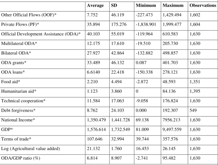
Table 1 presents some descriptive statistics of data used in the empirical analysis. All the data are expressed in real term and per capita. On average in the sample, GDP per capita and NI per capita are respectively about 1,576 USD and 1,350 USD. External financial flows are much smaller. On average, other official flows are 7 USD, private flows 35 USD and net ODA per capita 40 USD. Net ODA is characterized by the importance of the bilateral part for

10

According to the Development Assistance Committee glossary, programmable aid reflects the amount of aid that can be programmed by the donor at partner country level. It is defined through exclusions, by subtracting from total ODA unpredictable aid by nature (humanitarian aid and debt forgiveness and reorganization), no cross-border flows (development research in donor country, promotion of development awareness, imputed student costs, refugees in donor country and administrative costs), aid that is not part of co-operation agreements between governments (food aid and aid extended by local governments in donor countries), aid that is not programmable by the donor (core funding to national NGOs and International NGOs) or that is not susceptible for programming at country level (e.g. contributions to Public Private Partnerships, for some donors aid extended by other agencies than the main aid agency). A long series of programmable aid is unfortunately not available.

(13)

12

27 USD and grants for 33 USD. Debt forgiveness constitutes, on average, a quarter of grants. In addition, official assistance represents a small fraction of GDP (on average 6.8%). This implies that the expected stabilization achieved through aid is necessarily limited. However, a closer look reveals that a significant number of countries are highly dependent on aid. About a quarter of countries, the poorest in the sample, have their Aid/GDP ratio higher than 10%. For instance, in Mozambique, the most aid dependent in our sample, has received on average from 1981 to 2006 32% of GDP. Therefore, stabilization realized by aid might be important in such countries and relevant for donor aid policies.

Table 1: Descriptive statistics

Average SD Minimum Maximum Observations

Other Official Flows (OOF)* 7.752 46.119 -227.473 1,429.494 1,602

Private Flows (PF)* 35.894 175.276 -1,838.901 1,999.477 1,604

Official Development Assistance (ODA)* 40.103 55.019 -119.964 610.583 1,630

Multilateral ODA* 12.175 17.610 -19.510 205.730 1,630 Bilateral ODA* 27.927 42.864 -132.882 498.857 1,630 ODA grants* 33.489 46.132 0.087 401.703 1,630 ODA loans* 6.6140 22.418 -150.338 278.121 1,630 Food aid* 2.210 4.494 -2.872 48.593 1,351 Humanitarian aid* 1.123 3.860 0 84.136 1,395 Technical cooperation* 11.584 17.063 -9.058 176.824 1,630 Debt forgiveness* 8.762 24.103 0.000 192.307 549 National Income* 1,350.479 1,441.728 69.138 7956.213 1,630 GDP* 1,576.614 1,732.549 81.009 9,497.559 1,630 Terms of trade* 107.646 32.994 39.744 357.576 1,630

Log (Agricultural value added) 21.132 1.760 16.453 26.145 1,630

ODA/GDP ratio (%) 6.814 8.907 -2.741 95.482 1,630

*Data are in constant 2000 USD and in per capita terms. SD is the standard deviation.

3.2 Panel analysis

(14)

13

volatile and destabilizing in recipient countries. We find that official flows and mostly official development assistance does cope with a sizeable fraction of GDP shocks, stabilize available resources and thereby could be used as an insurance device in developing countries.

We estimate for the whole sample the contribution of ODA to resource stabilization as presented in equation (6). Both OLS and IV results are reported in Table 2. The IV estimates are generally robust. For instance, in the first stage, the R-squared is reasonable (0.435) and the F-statistic is significant at 1% (Table 2, column [2]). The estimated coefficients indicate that the fraction of GDP shocks smoothed out is 13.2% with the OLS (significant at 10%) and 13% with the IV (significant at 1%).

We do an in-depth analysis on the contribution of net ODA according to donors and the extent of aid concessionality. We compare ODA provided by bilateral donors to the ODA provided by multilateral agencies. Results indicate that, in line with its relative important size, bilateral aid is more stabilizing than the multilateral aid. Estimated coefficients for bilateral and multilateral ODA are robust (Table 3, columns [1]-[4]). Bilateral ODA contributes to ease 9.5% (OLS) and 8% (IV) of shocks, whereas multilateral aid only smoothes out 5% (OLS) and 5.6% (IV) of shocks.

Next, we contrast the contributions of ODA grants and ODA loans. In Table 4, the comparison of columns [1] and [2] to columns [7] and [8] reveals that, as expected, the stabilizing property of foreign assistance is attributed to concessional loans. ODA loans smoothed out 7.5% (OLS) and 11.4% (IV) of GDP shocks. Contrary to concessional loans, the estimated coefficients for grants are positive but not significant. However, when debt forgiveness is excluded, grants are as stabilizing as ODA loans (Table 4, column [4]). As anticipated in columns [5] and [6], debt forgiveness could be destabilizing in the extent that it would really increase available resources.

Furthermore, as previously noted, net ODA covers heterogeneous flows. Some components are imputed but not really transferred to recipient countries. We also separate emergency flows, as they are naturally countercyclical. Therefore we exclude humanitarian aid, food aid and technical cooperation from aid figures. Results in Table 5 indicate that excluding the automatic countercyclical aid components and the no cross-border elements, aid is significantly stabilizing for 15.8% of GDP shocks with the OLS and 9.9% with the IV. When moreover we subtract debt forgiveness, the β-coefficient is even higher (23-24% of GDP

(15)

14

shocks are stabilized), but we must note that according to the Hansen-Sargan test the instrumentation is no more valid.

Placed side by side to other financial flows toward developing countries, foreign aid appears remarkably stabilizing. With the purpose of making a comparison, we conduct a similar analysis for other official flows (OOF) and private flows (PF). We obtain that official flows are usually stabilizing, whereas private flows are destabilizing. Resource stabilization obtained from net OOF is relatively low. They contribute to absorb 2.2% with the OLS and 3% with the IV (Table 6, columns [1] and [2]). Net ODA and net OOF jointly smooth out about 15% of output shocks. Radically different from official flows, net private flows are destabilizing. The estimated coefficient in Table 6, columns [3] and [4] is between -6.3% (OLS) and -7.5% (IV).

Table 2: Official Development Assistance

Official Development Assistance (ODA)

OLS IV [1] [2] Coefficient β 0.132* 0.130*** (0.068) (0.035) First stage R2 0.435 F-statistic Sig. Hansen-Sargan probability 0.59 Observations 1630 1548 Countries 78 78

OLS: Ordinary Least Squares; IV: the first difference of GDP is instrumented by its one period lagged value and by the first difference of terms of trade and agricultural value added. Sig.: The F-statistic is significant at 1%. Estimates are corrected for potential autocorrelation AR (1) and for heteroskedasticity. Robust standard errors in parentheses, * significant at 10%; ** significant at 5%; *** significant at 1%.

(16)

15 Table 3: Bilateral ODA and multilateral ODA

Bilateral ODA Multilateral ODA

OLS IV OLS IV [1] [2] [3] [4] Coefficient β 0.095* 0.080*** 0.050** 0.056** (0.052) (0.018) (0.024) (0.025) First stage R2 0.475 0.472

F-statistic Sig. Sig.

Hansen-Sargan probability 0.04 0.84

Observations 1629 1548 1629 1548

Countries 78 78 78 78

(17)

16 Table 4: ODA Grants and ODA Loans

ODA Grants Debt forgiveness (a) ODA Loans

With debt forgiveness Without debt forgiveness

OLS IV OLS IV OLS IV OLS IV

[1] [2] [3] [4] [5] [6] [7] [8]

Coefficient β 0.074 0.044 0.122 0.125*** -0.096** -0.161*** 0.075*** 0.114***

(0.068) (0.034) (0.076) (0.038) (0.036) (0.061) (0.021) (0.031)

First stage

R2 0.468 0.388 0.512 0.555

F-statistic Sig. Sig. Sig. Sig.

Hansen-Sargan probability 0.61 0.33 0.46 0.05

Observations 1630 1548 1630 1548 557 549 1630 1548

Countries 78 78 78 78 48 48 78 78

(a): Only 48 states in the sample have benefited from debt forgiveness according to the DAC data. Here, we consider countries with missing figures have not benefited debt cancellation, i.e. missing figures are not missing observations. OLS: Ordinary Least Squares; IV: the first difference of GDP is instrumented by its one period lagged value and by the first difference of terms of trade and agricultural value added. Sig.: The F-statistic is significant at 1%. Estimates are corrected for potential autocorrelation AR (1) and for heteroskedasticity. Robust standard errors in parentheses, * significant at 10%; ** significant at 5%; *** significant at 1%.

(18)

17 Table 5: Total ODA corresponding to real transfers

With debt forgiveness Without debt forgiveness

OLS IV OLS IV [1] [2] [1] [2] Coefficient β 0.158** 0.099*** 0.242*** 0.235*** (0.078) (0.025) (0.079) (0.055) First stage R2 0.524 0.532

Observations 981 943 981 943

Real transfers are computed as total ODA excluding humanitarian aid, food aid and technical cooperation. OLS: Ordinary Least Squares; IV: the first difference of GDP is instrumented by its one period lagged value and by the first difference of terms of trade and agricultural value added. Sig.: The F-statistic is significant at 1%. Estimates are corrected for potential autocorrelation AR (1) and for heteroskedasticity. Robust standard errors in parentheses, * significant at 10%; ** significant at 5%; *** significant at 1%.

(19)

18 Table 6: Other Official Flows, Private Flows

Other Official Flows (OOF) Private Flows (PF)

OLS IV OLS IV [1] [2] [3] [4] Coefficient β 0.022** 0.030** -0.063*** -0.075*** (0.009) (0.014) (0.015) (0.023) First stage R2 0.552 0.563

Observations 1593 1516 1604 1523

3.3 Cross-country analysis

In order to provide insights into the stabilization property of official aid, we explore determinants of the contribution of aid to resource stabilization. We first analyze the economic vulnerability of recipient states. Donors may be incited in providing more stabilizing aid flows to countries exposed to frequent exogenous shocks. It is then logical to anticipate that stabilization achieved through official aid would be positively associated with the volatility of output. Second, we examine some features of aid disbursements according to each country. In aid dependent countries, a marginal change in the timing of aid flows may be more effective in addressing exogenous shocks. For that reason, we may postulate that aid dependency is a crucial determinant of the contribution of aid to stabilization. Third, we include the speed of aid disbursements in the list of determinants of stabilizing aid. After an output shock, a rapid disbursement is likely to be suitable to an output shock and then to foster the stabilizing impact of aid inflows; inversely, lags in aid disbursement may prevent rapid and countercyclical disbursement. The speed of disbursements depends on the sector financed by aid. For instance, supports to government budgets are more flexible and rapidly

(20)

19

disbursed than project aid. Finally, the volatility of aid flows is commonly presented as a source of unpredictable revenue and of macroeconomic instability. In fact, the anticipated impact of aid volatility is ambiguous: as previously noticed, countercyclical or procyclical aid flows are stabilizing when their fluctuations are lesser than the fluctuations of recipient output, i.e. aid varies less than output.

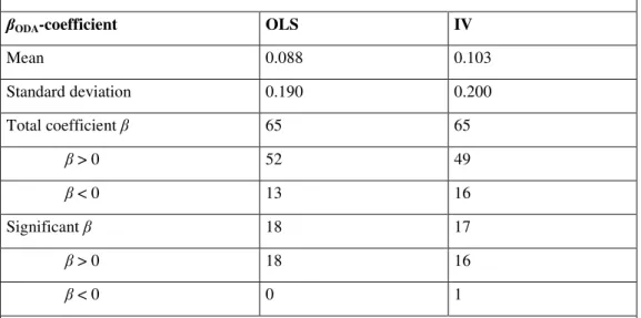
We first estimate equation (6) for each country with more than 10 observations in the sample. We present descriptive statistics on

β

ˆ_i_,_ODA coefficients in Table 7. We are able to estimate 65 β-coefficients from which 18 with the OLS and 17 with the IV are significant at least at 10%. The estimated coefficients are mostly positive indicating that aid is generally stabilizing. On average, on

β

ˆi,ODA is 0.088 with the OLS estimates and 0.103 with the IV.

Table 7: Descriptive statistics on βODA-coefficient by country

βODA-coefficient OLS IV

Mean 0.088 0.103 Standard deviation 0.190 0.200 Total coefficient β 65 65 β > 0 52 49 β < 0 13 16 Significant β 18 17 β > 0 18 16 β < 0 0 1

The significance is defined at the level of 10%.

After then, we analyze possible determinants through the following regression:

i ki k ODA , i X ˆ

_α

_ϕ

_ε

β

= +

∑

+ (7) ODA , i ˆ

β

is the estimated coefficient for the recipient country i from equation (6). The variables

ki

X denote the country determinants of the stabilization property of aid, i.e. output volatility, aid dependency, aid volatility or lags. The volatility of output and aid are respectively

(21)

20

computed as the standard deviation of the growth rate of GDP per capita and the growth rate of net ODA per capita. Aid dependency is calculated as the average of the aid output ratio. The speed of aid disbursements is approximated by the average of the yearly ratio of net ODA disbursements on ODA commitments. We also control for some structural factors such as colonial relationships between donor and recipient countries (British and French colonization dummies), geographical handicaps (Landlocked and Island dummies) and geographical locations (African, American and Asian dummies). We also add a dummy for the significance at least at 10% of the coefficients

β

ˆ_i_,_ODA. The

ϕ

_k are coefficients to be estimated. The

ε

_i

represent the error terms. We estimate equation (7) with the simple OLS.

We report results in Table 8. Whatsoever the estimation, we find that foreign official aid tends to be more stabilizing in countries facing important output fluctuations and particularly dependent on aid. The volatility of GDP and the dependency on aid significantly increase the estimated coefficient

β

ˆ_i_,_ODA. The effects of aid volatility and disbursement speed are insignificant. We also obtain that aid stabilization is not significantly affected by colonial relationships and geographical handicaps. Likewise, geographical location is not a key determinant in the stabilization property of aid, except for Latin American countries with the IV estimates.

(22)

21 Table 8: Determinants of aid stabilization.

βODA-coefficient OLS IV

[1] [2] [3] [4] [5] [6] [7] [8] GDP volatility 3.440** 2.752* 3.492** 2.880* 3.261** 2.634** 3.319** 2.744** (1.550) (1.523) (1.519) (1.498) (1.315) (1.256) (1.288) (1.188) Aid dependency 1.061** 1.144** 1.011** 1.111** 1.398*** 1.529*** 1.353*** 1.510*** (0.502) (0.489) (0.487) (0.485) (0.467) (0.409) (0.468) (0.406) Speed of disbursements -0.053 -0.051 -0.122 -0.117 -0.100 -0.126 -0.169 -0.214 (0.131) (0.121) (0.157) (0.148) (0.153) (0.146) (0.187) (0.187) Aid volatility -0.055 -0.020 -0.066 -0.034 -0.007 0.035 -0.018 0.019 (0.119) (0.116) (0.111) (0.106) (0.099) (0.101) (0.098) (0.099) French or British colonization 0.100 0.119* 0.037 0.100 (0.069) (0.069) (0.067) (0.074) French colonization 0.079 0.095 0.016 0.070 (0.067) (0.067) (0.073) (0.081) British colonization 0.129 0.144* 0.065 0.137* (0.082) (0.082) (0.078) (0.076) Geographical handicap (Landlocked or Island) 0.043 0.025 0.048 0.027 (0.049) (0.050) (0.048) (0.052) Landlocked 0.078 0.051 0.082 0.053 (0.067) (0.071) (0.064) (0.064) Island -0.027 -0.026 -0.018 -0.034 (0.033) (0.033) (0.047) (0.051) Africa -0.011 -0.037 -0.030 -0.046 0.023 -0.031 0.005 -0.041 (0.102) (0.091) (0.079) (0.075) (0.057) (0.064) (0.052) (0.063) America 0.149 0.110 0.130 0.102 0.146** 0.136** 0.129** 0.126** (0.112) (0.099) (0.090) (0.084) (0.070) (0.063) (0.062) (0.057) Asia 0.113 0.047 0.092 0.034 0.115** 0.060 0.095** 0.037 (0.101) (0.100) (0.076) (0.081) (0.055) (0.063) (0.043) (0.053) Significance dummy 0.118*** 0.109** 0.149** 0.152** (0.042) (0.047) (0.063) (0.061) Constant -0.182 -0.178 -0.104 -0.112 -0.148 -0.153 -0.072 -0.069 (0.174) (0.173) (0.145) (0.145) (0.156) (0.162) (0.160) (0.175) Observations 65 65 65 65 65 65 65 65 R2 0.27 0.34 0.31 0.36 0.35 0.43 0.37 0.46

(23)

22

Robust standard errors in parentheses, * significant at 10%; ** significant at 5%; *** significant at 1%.

4 Conclusion

There is growing debate on the consequences of aid volatility. More than a few authors have argued that aid is an important source of macroeconomic instability in developing countries: aid is volatile, unpredictable and frequently procyclical, i.e. it is generally disbursed during an expansion period in recipient countries and postponed or suspended during downturn periods. However, the proposal that volatile aid generates or exacerbates shocks is debatable. Volatile aid is not problematic if it contributes to the coping with exogenous shocks in developing countries. Stabilizing aid is by definition volatile. Procyclical or countercyclical aid could ease output shocks depending on the size of its instability. Analyzing stabilizing aid is then more relevant than analyzing volatile or cyclical aid.

This article studies whether or not aid is stabilizing. We estimate to what extent official assistance copes with exogenous output shocks in recipient countries and stabilizes resources available for the financing of consumption, investment and net trade. Contrary to private flows, net ODA does stabilize available resources against GDP shocks whatever the ODA disaggregation (bilateral ODA vs. multilateral ODA, and ODA grants vs. ODA loans). Total ODA contributes to smooth out 13% of output shocks while ODA flows corresponding to real transfers cope with 24% of shocks. Further, stabilizing aid is more effective in countries subject to frequent output fluctuations and countries that are highly dependent on aid.

If the objective is to stabilize income in developing countries, donor community might enhance this property of aid as an insurance device. Stabilizing aid must be disbursed to vulnerable and aid dependent countries. This last conclusion contrasts with the common idea that aid scaling-up could be a source of growing macroeconomic instability in developing countries (see for instance IMF 2005 or World Bank Global Monitoring Report 2005 and 2006). Most notably, our estimates also indicate that bilateral aid mainly explains stabilizing aid. Therefore, multilateral agencies have to focus on the design of stabilizing official assistance. Actually, multilateral official assistance is mostly driven by good economic and social policies. Indeed, the “Country Policy and Institutional Assessment” (CPIA) computed by multilateral organizations (World Bank and others) is the predominant criterion in the

(24)

23

allocation formula of multilateral development banks. Therefore it would be relevant to introduce in these allocation formulas a measurement representing economic vulnerability of recipient countries (Guillaumont 2008). Taking into consideration the structural vulnerability of countries in the allocation of aid appears urgent as the present global financial and economic crisis has detrimental consequences on developing countries.

References

Afonso, A., and D. Furceri (2008) “EMU Enlargement, Stabilization Costs and Insurance Mechanisms,” Journal of International Money and Finance, 27 (2), pp. 169-187.

Arreaza, A., B. E. Sorensen, and O. Yosha (1998) “Consumption Smoothing through Fiscal Policy in OECD and EU Countries,” Working Paper 6372, National Bureau of Economic Research (NBER).

Asdrubali, P., and S. Kim (2004) “Dynamics Risk sharing in the United States and Europe,”

Journal of Monetary Economics, 51, pp. 809-836.

Asdrubali, P., B. Sorensen and O. Yosha (1996): “Channels of Interstate Risk Sharing: United States 1963-90,” Quarterly Journal of Economics, 111 (4), pp. 1081-1110.

Bayoumi, T. (1999): “Interregional and International Risk Sharing and Lessons for EMU: A Comment,” Carnegie-Rochester Conference Series on Public Policy, 51, pp. 189-193.

Bulir, A. and A. Hamann (2003): “Aid Volatility: An Empirical Assessment” IMF Staff

Papers, 50 (1), pp.64-89.

Bulir, A. and A. Hamann (2008): ‘Volatility of Development Aid: From the Frying Pan into the Fire?,’ World Development, 36(10), pp. 2048-2066.

Burnside, C. and D. Dollar (2000): “Aid, Policies, and Growth,” American Economic Review, 90(4), pp. 847-868.

Clemens M. A., S. Radelet and R. Bhavnani, 2004, “Counting Chickens When They Hatch: The Short Term Effect of Aid on Growth,” Working Paper. 44, Center for Global

Development.

Collier P. and J. Dehn (2001), “Aid, Shocks and Growth” World Bank Policy Research Working Paper, N° 2688. Washington D.C.

(25)

24

Collier, P. and Dollar, D. (2002): “Aid Allocation and Poverty Reduction,” European

Economic Review, 46(8), 45(1), pp. 1475-15001-26.

Da Rocha, J. M. and D. Restuccia (2006): “The Role of Agriculture in Aggregate Business Cycles,” Review of Economic Dynamics, 9(3), pp. 455-482.

Fielding, D. and G. Mavrotas (2008): “Aid Volatility and Donor-Recipient Characteristics in ‘Difficult Partnership Countries’,” Economica, 75(299), pp. 481-494.

Gemmell, N. and M. McGillivray (1998): “Aid and Tax Instability and the Government Budget Constraint in Developing Countries”, CREDIT Research Paper 98/1, University of Nottingham.

Guillaumont, P. (2008): Adapting Aid Allocation Criteria to Development Goal. An essay for the 2008 Development Cooperation Forum, United Nations Economic and Social Council. Guillaumont, P. and L. Chauvet (2001): “Aid and Performance: A Reassessment,” Journal of

Development Studies, 37(6), pp. 66-92.

Guillaumont, P. and L. Chauvet (2009): “Aid, Volatility and Growth Again. When Aid Volatility Matters and When it does not,” Review of Development Economics, 13(3).

Gupta, S., B., Clements and E. R. Tiongson (2004): “Foreign aid and Consumption Smoothing: Evidence from Global food aid,” Review of Development Economics, 8, pp. 379-390.

Hudson, J. and P. Mosley (2008): “Aid Volatility, Policy and Development,” World

Development, 36(10), pp. 2082-2102.

IMF (2005): “The Macroeconomic of Managing Increased Aid Inflows: Experiences of Low-Income Countries and Policy Implications”, prepared by the Policy Development and Review Department, August 8, 2005.

Kose, M. A. (2002): “Explaining Business Cycles in Small Open Economies: How Much Do World Prices Matter?,” Journal of International Economics, 56, pp. 299-327.

Lensink, R. and O. Morrissey, (2000): “Aid Instability as a Measure of Uncertainty and the Positive Impact of Aid on Growth,” Journal of Development Studies, 36(3), pp. 31-49.

Mélitz, J. and F. Zùmer (1999): “Interregional and International Risk Sharing and Lessons for EMU,” Carnegie-Rochester Conference Series on Public Policy, 51, pp. 149-188.

(26)

25

Fluctuations,” International Economic Review, 36, pp. 101-137.

Pallage, S. and M. Robe (2001): “Foreign aid and the Business Cycle,” Review of

International Economics, 9(4), pp. 641-672.

Pallage, S. and M. Robe (2003): “On the Welfare Cost of Economic Fluctuations in Developing Countries,” International Economic Review, 44(2), pp. 677-69.

Pallage, S., A. Robe and C. Bérubé (2006): “On the Potential of Foreign aid as Insurance”,

IMF Staff Papers, 53 (3), pp. 453-475.

Sorensen, B. and O. Yosha (1998): “International Risk Sharing and European Monetary Unification,” Journal of International Economics, 45, pp. 211-238.

(27)

26 Appendix 1: List of countries

78 developing and transition countries from 1981 to 2006 Africa (37) Algeria (1981-2005) Mozambique (1985-2006) Angola (1987-2006) Niger (1981-2003) Benin (1981-2005) Nigeria (1981-2005) Botswana (1981-2006) Rwanda (1981-2006) Burkina Faso (1981-2006) Senegal (1981-2006) Burundi (1981-2005) Seychelles (1986-2006) Cameroon (1981-2006) South Africa (1995-2006) Ca!pe Verde (1988-2006) Sudan (1981-2006) America (22) Argentina (1981-2006) Bolivia (1981-2006) Brazil (1981-2006) Chile (1981-2006) Colombia (1981-2006) Costa Rica (1981-2006) Dominican Republic (1981-2006) Ecuador (1981-2006) El Salvador (1981-2006) Grenada (2001-2005) Guatemala (1981-2006) Guyana (2001-2005) Honduras (1981-2006) Jamaica (2001-2006) Mexico (1981-2006) Nicaragua (1995-2006) Asia (16) Bangladesh (1981-2006) Cambodia (2001-2006) China (1981 (2006) India (1981-2005) Indonesia (1982-2006) Malaysia (1981-2006) Mongolia (2001-2006) Nepal (2001-2006) Pakistan (1981-2006) Philippines (1981-2006) Sri Lanka (1981-2006) Thailand (1981-2006) Jordan (1981-2006) Lebanon (2001-2006) Oman-2001-2004) Turkey (1981-2006)

(28)

27

Congo, Dem. Rep. (1981-2006) Swaziland (1981-2006) Equatorial Guinea (2001-2006) Tanzania (1991-2006) Ethiopia (1994-2006) Togo (1981-2005) Gabon (1981-2006) Tunisia (1981-2006) Ghana (1981-2006) Uganda (1984-2006) Guinea (1988-2006) Zambia (1981-2006) Kenya (1981-2006) Zimbabwe (1981-2005) Lesotho (1981-2006) Madagascar (1981-2006) Malawi (1981-2006) Mali (1981-2006) Mauritania (1981-2006) Mauritius (1982-2006) Morocco (1981-2006) Panama (1982-2006) Paraguay (1991-2006) Peru (1981-2006) St. Lucia (2001-2005) Suriname (2001-2006) Uruguay (1984-2006) Pacific (3) Fiji (1981-2006)

Papua New Guinea (2001-2003) Samoa (2001-2006)

(29)

28 Appendix 2: Data sources

Data Source

Net ODA, net disbursement and current USD OECD DAC website

Net ODA, commitment and current USD Idem

Concessional loans, net disbursement and current USD Idem

Grants, net disbursement and current USD Idem

Multilateral ODA, net disbursement and current USD Idem

Bilateral ODA, net disbursement and current USD Idem

Humanitarian aid, net disbursement and current USD Idem

Food aid, net disbursement and current USD Idem

Technical cooperation, net disbursement and current USD Idem

Debt forgiveness, net disbursement and current USD Idem

Other official flows, current USD Idem

Private flows, current USD Idem

Consumption of fixed capital/GNP (%) World Development Indicators 2008

GDP, constant 2000 Idem

GDP, current USD Idem

GNP, current USD Idem

Population Idem

Terms of trade (net barter terms) basis 100 in 2000 Idem

Agricultural value added, constant 2000 USD Idem

British colonization Authors

French colonization Idem

Island Idem