HAL Id: halshs-00556809
https://halshs.archives-ouvertes.fr/halshs-00556809
Preprint submitted on 17 Jan 2011
HAL is a multi-disciplinary open access archive for the deposit and dissemination of sci-entific research documents, whether they are pub-lished or not. The documents may come from teaching and research institutions in France or abroad, or from public or private research centers.
L’archive ouverte pluridisciplinaire HAL, est destinée au dépôt et à la diffusion de documents scientifiques de niveau recherche, publiés ou non, émanant des établissements d’enseignement et de recherche français ou étrangers, des laboratoires publics ou privés.
countries
Jean-Louis Combes, Samuel Guérineau, Pascale Combes Motel
To cite this version:
Jean-Louis Combes, Samuel Guérineau, Pascale Combes Motel. Deforestation and credit cycles in Latin American countries. 2011. �halshs-00556809�
Document de travail de la série
Etudes et Documents
E 2008.08
Deforestation and credit cycles in Latin American countries
Jean-Louis Combes, Samuel Guérineau, Pascale Combes Motel, CERDI-CNRS, Clermont Université
This version: June, 30 2008 27 p.
Corresponding and presenting author: P.Motel_Combes@u-clermont1.fr
CERDI-CNRS Clermont Université, 65 Bd F. Mitterrand, 63000 Clermont-Ferrand, France
Acknowledgments. The authors thank the organisers and participants of the 2008 AFSE Thematic
Meeting “Frontiers in Environmental economics and natural resources management” held in Toulouse (France), June 9-11, 2008. Comments from participants at the “environmental and resource economics” seminar from the Centre d’Economie de la Sorbonne are also acknowledged. The usual disclaimers apply.
Deforestation and credit cycles in Latin American
countries
Abstract
This paper establishes a link between deforestation and credit cycles in Latin American countries. The latter exhibit rapid deforestation rates as well as macroeconomic instability that is often rooted in credit booms and crunches episodes: data available on the last years show a coincidence between higher macroeconomic instability and deforestation increases. This paper provides a theoretical explanation and econometric investigations of this phenomenon.
A key ingredient of the model is the existence of two sectors: a modern agricultural sector and a subsistence one, which are hypothesised to catch the basic features of Latin American agricultural sectors. Agricultural production relies on three production factors: land, capital and labour. Agents clear forested areas in order to increase agricultural lands. Interest rates movements have an effect on agricultural decisions and thus on deforestation since they induce factor movements between the agricultural sectors. It is shown that deforestation occurs in response to interest rates increases or decreases primarily because of the irreversible character of forest conversion.
Econometric tests are conducted on the 1948-2005 period on an exhaustive sample of Latin American countries. The database on deforestation is a compilation of FAO censuses and several measures of credit cycles are calculated as well. The main output of the paper is to evidence a link between credit cycles and deforestation. The results are robust to the introduction of usual control variables in deforestation equations.
Keywords : Credit cycles, Deforestation, Latin America
1. Introduction
Latin American countries experience a rapid deforestation: annual average deforestation rates in the most recent periods are twice the world’s ones: 0.46% versus 0.22% over the 1990-2000 period and 0.51% versus 0.18% over the 2000-2005 period.1 Since primary forests in these countries account for 56% of the world’s primary forests, the Latin American paces of deforestation raise particular concern and emerge as an international issue related to global warming and loss of biodiversity.2 Forest preservation sustains the objectives of the United Nations Framework Convention on Climate Change Convention and delegates who met in Bali in late 2007 agreed to consider standing forests as a device against global warming. Latin American countries have expressed their interest in participating in a Forest Carbon Partnership Facility. Moreover, forest preservation in Latin American countries meets also the objectives of the Convention on Biological Diversity in as much as at least 10 Latin American countries have more than 1,000 native tree species (FAO, 2007) and a great amount of species extinction occurs in tropical environments (Myers, 1993).
National initiatives remain however important but rely on the understanding of the deforestation process which has been extensively studied. According to Geist and Lambin (2002), “source” or “proximate” causes of deforestation relate mainly to economic activities taking place at the local level such as investments in infrastructure and road networks (Angelsen, 1999; Chomitz & Gray, 1998), expansion of cattle ranching and agricultural activities (Barbier, 2004b) and finally commercial logging (Van Kooten & Folmer, 2004). Geo-ecological factors such as soil quality, rainfall and temperature conditions are considered as “predisposing” factors of deforestation which condition the links between “proximate” and “underlying” causes. The latter operate mainly at the macro level and are related to social processes and economic policies such as the population pressure (Bilsborrow & Carr, 2001; Cropper and Griffiths, 1994), landownership and income distributions, national and regional development strategies (Koop and Tole, 2001), agricultural research and technological change as well (Southgate et al. 1990). The poor quality of institutions tends to accompany deforestation. Weakness of property rights creates incentives to capture rents generated by forest extraction (Deacon, 1999). Inappropriate rules of law may incite forest dwellers to
1
These figures are not strictly comparable to the figures calculated in the paper (see Table 2 in the statistical appendix) since FAO’s deforestation rates are calculated by summing annual variations of forest areas. Moreover Mexico is not included in the figures reported by the FAO.
2
Climate change from forest conversion may also occur locally (Tinker, Ingram & Struwe, 1996) and preserving biodiversity also yields domestic benefits (Chomitz & Kumari, 1998)
become agents of deforestation (Southgate & Runge, 1990). Moreover, bribes and agricultural lobbies generate rural subsidies that both encourage low agricultural productivity and deforestation (Bulte, Damania and López, 2007).
Other studies have highlighted the role played by macroeconomic - fiscal, exchange rate and / or sectoral - policies in the deforestation process (e.g. Anderson, 1990). Exchange rate depreciation promotes exporting sectors and by the way forest conversion. Exchange rate variations may however have an ambiguous impact on deforestation, depending on their permanent or transitory patterns (Arcand et al. 2007). The terms of trade affect deforestation of timber exporting countries. An improvement in the terms of trade may be the result of an increasing demand for timber products. If a country relies on its export earnings, an increase in the terms of trade will reduce the long term forest stock (Barbier & Rauscher 1994). Openness may however dampen the effect of population pressure on forests when giving new opportunities for the economy (Hecht et al. 2006). Debt is also an important issue for deforestation in developing countries. Debt can induce myopic behaviours and foster forest depletion especially when a country must meet its international financial commitments (Culas, 2006). However debt for nature swaps may impede such a process (Kahn & Mac Donald, 1994). The evidence for Latin American countries is not however clear cut. Gullison and Losos (1993) assert that agricultural and timber exports did not increase with growing external debt. It is hard to isolate the peculiar role played by the external debt among other macroeconomic factors in land degradation in the 80’s. Moreover, debt repayments may have been responsible for drastic public spending reductions in infrastructures provision that have a positive effect on deforestation.
This paper provides further investigations into underlying causes related to a peculiar macroeconomic feature of Latin American countries. For many years, the latter are subject to credit cycles defined as successive expansion and slowdown phases in the supply of credit and thus in its opportunity cost. Latin American countries experienced credit stagnation in the late 90s (e.g. Barajas and Steiner, 2002), which coincides with an increase in deforestation rates. One can wonder whether there exists a causal relationship between credit cycles and deforestation. The ambiguous consequences of credit expansion on deforestation are examined in the literature. On the one side, credit allows financing investments in infrastructures that boost deforestation (Pacheco, 2006; Ferraz, 2001; Culas, 2003). On the other side credit facilitates the adoption of intensive agriculture which is less forest consuming (Angelsen, 1999; Caviglia-Harris, 2003). This paper concentrates rather on the
consequences of credit cycles. Credit cycles are deemed to modify relative prices, and thus are expected to influence resources allocation between sectors in accordance with their capital intensities. It is argued that both credit expansions and credit crunches may have positive effects on deforestation i.e. credit cycles foster deforestation. This proposition is formalized with a two sectors model which posits a modern agricultural sector and a subsistence one. This dual economy model is hypothesised to catch the basic features of Latin American economies which exhibit a deforestation path in the long run. Agricultural production relies on three production factors: land, capital and labour. Economic agents clear forested areas in order to increase their land plots. Interest rates movements pour financial instability into agricultural decisions. It is shown that deforestation occurs in response to interest rates increases and decreases as well primarily because of the irreversible character of primary forest conversion.
The remainder of the paper is organized as follows. Section 2 puts forwards stylised facts relating deforestation and credit cycles in Latin America. Section 3 offers a theoretical framework of the engines of deforestation. Section 4 provides some econometric results and Section 5 concludes.
2. Deforestation and credit cycles in Latin American countries
2. 1. Why focusing on credit cycles effects?
Latin American countries have experienced pronounced credit cycles characterised by phases of strong acceleration of credit growth (credit or lending booms) followed by a drastic reduction in credits (credit crunches) from world war II onwards (e.g. Caballero, 2000; Gourinchas, Valdés, & Landerretche, 2000). The first three decades (50s to 70s) are marked by a rapid credit expansion, with several deceleration episodes (see Figure 1 in the statistical appendix). Tight credit policies in the 80s are combined with financial repression in the aftermath of the debt crisis. The financial liberalisation in the late 80s spurred a credit expansion in the early 90s followed by a credit stagnation episode since the late 90s (Barajas & Steiner, 2002). More generally, credit cycles either occur with economic policies reversals (e.g. the brazilian experience of tight credit against inflation in the 60s - Randall, 1997; or the adoption of the Basel Accord in the 90s – Barajas et al. 2004) or international liquidity availability as well (e.g. petrodollars in the 70s – Amado et al., 2006). Braun and Hausmann (2002) show that the frequency of credit crunches is higher in Latin America than in other developing countries; moreover these credit crunches are deeper in magnitude and relatively
long-lived. They also argue that the recent episodes of credit crunches have been more frequent and severe than before. Credit cycles are thus a prominent feature of Latin American countries for many years and are a key ingredient of their macroeconomic instabilities.
Why Latin American countries are particularly prone to these credit crunch and credit boom periods? Three pieces of explanation can be put forward and are related to (i) financial markets characteristics, (ii) exchange rate shocks and currency crises, and (iii) monetary policies.
Poor financial development3 is a salient character of Latin American countries (Caballero, 2000 among others).4 This was the case from the 50s until the late 80s, i.e. from state led to liberalised financial markets. Underdeveloped financial markets are prone to moral hazard. A poor banking supervision leads depositors to withdraw their funds in periods of recession. Moreover, economic agents have a limited access to collaterals due to the poor property rights especially on land. Therefore, moral hazard is exacerbated during economic crises and the collateral valuation has a pro-cyclical behaviour (Bernanke and Gertler, 1989). Latin American countries implemented financial liberalization after financial repression periods, in order to encourage financial deepening. The latter however created disturbances into credit markets and may be the ‘proximate’ cause of financial crises in the late 80s (Mas, 1995). Financial liberalization may thus have failed to eliminate moral hazard problems. The latter are spawned by persistent implicit or explicit bailout guarantees which exacerbate the tendency toward high risk projects (Caballero, 2000). Last, the operating costs of the financial system remain high in Latin American countries (Brock & Rojas Suarez, 2000).
The structure of balance sheets of Latin American firms raises their vulnerability to exchange rate shocks. A currency mismatch occurs when an entity’s net worth or income is sensitive to changes in the exchange rates. The asset is labelled in the local currency but the mortgage in dollars (stock aspect); the incomes generated by the asset are in the local currency but the repayments are due in dollars (flow aspect). The net present value of investments financed by foreign funds is sensitive to exchange rates fluctuations independently of the fundamental parameters of the investment project. Therefore, the banks’ liquidity and then their credit supply are affected by exchange rate fluctuations.
3
It is measured by M3 to GDP or loans to private sector to GDP. 4
One exception is Chile which is however characterised by a thin financial market which leverages interest rates movements (Caballero, 2004)
At last, the size and frequency of credit cycles may be explained by the weakness of countercyclical policies. For instance, Latin American countries have hardly implemented countercyclical monetary policies. Capital controls allow theoretically countercyclical monetary policies under a fixed exchange rate regime. Such a situation was prevalent in Latin American countries from the 50s to the 80s, but populist regimes were very reluctant to rely on that kind of policy. At last, the adoption of floating exchange rates does not allow strong countercyclical monetary policies due to the “Original sin” effect (Eichengreen, Hausmann, and Panizza, 2003). Indeed, when countries borrow in dollars, exchange rates movements may have large wealth effects. In this context Central Banks can hardly prevent liquidity crises since base money issues would lead to a huge increase of the debt service through exchange rate depreciation.
Admittedly, credit cycles are associated with business cycles but one may easily think about sectoral effects as well. It is argued here that credit cycles are of peculiar importance for environmental issues for different reasons. First, credit cycles are considered to be symptoms of financial constraints (e.g. Caballero 2000) i.e. to be closely linked with credit rationing which is still perceived by rural households despite ‘market friendly’ reforms in the agricultural sector (Boucher et al. 2005). In such a situation, credits are allocated mainly to large landowners who can justify substantial collaterals i.e. lands, consume relatively more land and thus are more readily able to clear the forest (Southgate and Whitaker, 1998). Second, credit cycles spur on asset prices and thus land prices variations which may affect deforestation. Third, credit cycles may be the pretext to public interventions aimed at providing peculiar public goods like forested lands or subsidized credits to the agricultural sector. In this paper it is argued that interest rates’ movements also have an effect on deforestation through factor reallocations within the agricultural sector.
2. 2. Patterns of deforestation in Latin America
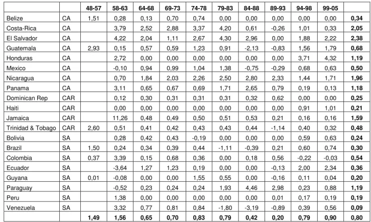
Annual deforestation rates between 1948 and 2005 are reported in Table 3 in the statistical appendix from available FAO censuses.5 Data frequency on forests allows calculating only period averages on the beginning of the time period. At the end of it, although annual data are available, period averages are calculated since annual data are often interpolations. 20 countries are included in the sample within each period, except the first one where forest
5
coverage statistics are only available in 7 countries.6 Among the 20 Latin American countries included in the sample, there are 4 Caribbean, 7 Central American and 9 South American countries. Deforestation rates in Latin American countries differ sharply across space. A simple and preliminary decomposition of the deforestation process show that idiosyncratic factors are at work. This can be shown by estimating a regression equation of average annual deforestation rates on periods and country fixed effects. The magnitude of idiosyncratic factors may be inferred from the calculation of 1-R2 of the regression. The latter is 0.82 which must be interpreted as an upper bound on the variance of independent idiosyncratic factors since the total variability may also be the result of measurement errors.
Deforestation rates are high during the 50s, the 60s and the 70s, then drop in the 80s and increase sharply since the second half of the 90s. High rates of deforestation in the 50s and 60s did not raise particular concern in this post-war period which was characterised by the overwhelming goal of economic growth and great optimism (Edwards, 1995). Large parts of primary forests disappeared with for instance the destruction of the Atlantic rainforest in Brazil due to coffee plantations expansions (Thorp, 1998). Import substitution strategies (ISS) have been conducted in the 50s and the 60s in many Latin American countries. Although they gave a non negligible importance to mining and forest products industries (Randall, 1997), it is considered that they reduced natural resource use by promoting industrial sectors. Nevertheless, despite the ISS’ anti-agricultural bias, it is alleged that ISS gave less incentives to conserve natural resources. For instance, land was under-utilized in large agricultural establishments of which lands may have encroached on forested areas and the management of environmental base in agriculture was more depletive (Barham et al. 1992; Southgate & Whitaker, 1992).
If we compare deforestation figures among countries, the highest deforestation rates are found in Central American countries. Among the seven countries that exhibit an average deforestation rate over the whole period greater than 1%, five are Central American countries.7 Costa Rica experienced for instance the highest rates from the fifties to the beginning of the eighties, illustrating the predominant views of economic development in
6
Among 24 potential Latin American countries, 3 countries are dropped (Chile, Surinam and Uruguay) since they exhibit a forestation profile throughout the period. Argentina is also dropped since deforestation has taken place only on the last 2 periods.
7
These countries are El Salvador, Costa-Rica, Honduras, Nicaragua, and Panama; the remaining countries being Jamaica and Paraguay.
Latin America: agri-business exportation sector, import substitution strategy until the structural adjustment programs which stopped deforestation in the early 80s. Since then, forest preservation initiatives have greatly reduced the pressure on forests (de Camino et al., 2000). The same story is at work in Nicaragua and Honduras which have considerably developed their beef exports. The proximity of the United States has stimulated the demand for agricultural and cattle products. The Latin American Agri-business Development (LAAD) Corporation is deemed to have contributed to the process when pouring large amounts of capital into Central American countries in the 60s.
2. 3. Is there really a link between deforestation and credit cycles
episodes?
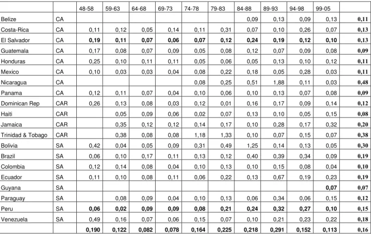
Once we have seen the importance and the main characteristics of credit and deforestation dynamics is there a way to put together these two series of stylized facts? First, there is no obvious correlation between the highest country average deforestation rates and the most pronounced credit cycles episodes. Among the seven countries having high deforestation rates, only one (Nicaragua) is also characterised by a strong credit instability as measured by standard errors of credit growth rates (see Table 4 in the statistical appendix). Second, the coincidence between periods of high deforestation and credit cycles is not clear-cut: it seems that credit booms are associated with an acceleration of deforestation, but this correlation is contradicted in the last period that is characterised by a tightening of credit and an increase in deforestation. This result is not surprising since many idiosyncratic factors affected credit cycles during the last decades. Among these factors it can be mentioned that financial reforms were implemented at different times (Edwards, 1995),8 but political factors played of course a prominent role.9 If we look at country-period data, the link between deforestation and credit cycles remains unclear: there is only 22% of coincidence between the highest deforestation figures and the highest credit growth rate instabilities.
Moreover, any simple correlation between deforestation speeds and credit growth rate instabilities must be cautiously interpreted. Indeed (i) simple correlations do not allow drawing causal links between deforestation and credit cycles, (ii) measuring credit cycles implies defining a long term or potential credit, and (iii) it is hard to disentangle the effects of the different stages within credit cycles (i.e. credit booms and credit crunches). These
8
Chile and Mexico were among the first reformers in the mid-80’s while Dominican Republic and Ecuador liberalised only in the mid-90’s.
9
difficulties elicit three constraints to test relevantly the existence of a causal relationship between deforestation and credit cycles: (i) the need to use multivariate regressions (ii) the need to define credit cycles as the gap between its current value and a trend, and (iii) the need to distinguish the impact of credit booms from credit crunches’ ones.
3. Deforestation model
Let us consider an agricultural economy made of two sectors.10 The first one is a “subsistence” sector and the second one is a “modern” sector. The subsistence sector has a production function G which uses land HG and labour LG only. Formal land property rights barely exist and impedes access to credit markets: capital accumulation cannot occur. Despite all these constraints, economic agents are deemed to maximise their profits according to the “poor but efficient” hypothesis (Schultz, 1964). It is hypothesised that the subsistence sector is representative of shifting or “slash and burn” agriculture. It consists in periodic clearing of forested areas for short periods of cultivation interrupted by long fallow periods which are essential for fertility restoration, weeds control and forest regeneration (secondary or degraded forest) purposes. Population pressure reduces fallow periods and generates deep advances in forested areas (Metzger, 2003). The modern sector has a production function F depending on three production factors: land HF, labour LF that equals L-LG, and capital K. Property rights are well defined and secured and capital can be accumulated since economic agents can use land as collateral. The modern sector pictures agricultural and or livestock-keeping activities that may have an access to formal and or international agricultural markets. The modern sector output is sold at price p; the numéraire is the output price of the subsistence sector.
Both production functions have positive and decreasing marginal productivities, and non increasing returns to scale. They satisfy Inada conditions and allow factors substitutions. In addition, cross second derivatives are non negative. Labour moves freely from one sector to another one with a constant total supply L. Both sectors share a common wage w that induces labour allocation in the economy. Capital use is determined by its opportunity cost r which includes a rental rate and an agency cost. Land is a specific factor of which prices are hG and hF in the subsistence and modern sectors respectively. It is assumed that land markets are poorly developed. Hence hG and hF represents clearing marginal costs, opportunity costs
10
Many researchers emphasised the dual character of Latin American agriculture (e.g. Dorner & Quiros, 1973; Horowitz, 1996)
generated by forest depletion and conflict costs within local populations. The land factor specificity is determined by localization, soil quality, and legal statute differences. For example, people concerned by subsistence (or traditional) agriculture, are located in the forest whereas modern agricultural activities take place rather in pioneer fronts. This specificity implies that land input variations in one sector are not compensated by opposite variations in the other.
Tropical rainforest is mainly considered as a non renewable resource. Hence, deforestation is an irreversible process which is mainly the result of agricultural land encroachments (FAO, 2007) from the subsistence and modern sectors. Increases in HF or HG are defined as deforestation (e.g. Barbier and Burgess, 2001) whereas decreases in HF or HG are increases of fallow lands or degraded forests. Fallow lands provide several products and services and allow raising cattle which increases the value of land (Fujisaka et al. 1996). It may be thus profitable even in the modern sector, not to reduce them under increasing demand for agricultural land.
Two models are presented. The first one allows land input adjustments in the modern sector. This hypothesis is relaxed in the second one. Land fixity in the modern sector can be justified in three ways. Modern agriculture is not land extensive: agricultural output increases can be the result of capital and / or labour increases. Legal constraints may also prevent land extensions in this formal sector. Moreover, land encroachments in tropical rainforest may be prohibitive: lack of infrastructures, clearing costs, costly land improvements in cleared areas. In the second model, the subsistence sector is the only cause of deforestation. For instance, in Central America capital intensive agricultural establishments had few impacts on forest resources. Forest clearance was mainly the result of increased pressure generated by subsistence farmers in areas endowed with a rich biodiversity and forests (Carr et al. 2006).
3. 1. Two engines of deforestation: modern and subsistence
sectors’ expansions
In a context where land is a choice variable in both sectors, the profit maximization is made upon HF, HG, LG and K:
(
G G)
(
G F)
G G F F H H K L H h H h rK wL K H L L pF H L G F G G,max, , π≡ , + − , , − − − −Subscripts indicate first derivatives and stars the optimum values in the first order necessary conditions: 0 * = ∂ π ∂ G L ⇔
(
,)
(
, ,)
0 * * * * * − − = K H L L pF H L G G F L G G L (1) 0 * = ∂ π ∂ K ⇔(
, ,)
0 * * * − = −L H K r L pFK G F (2) 0 * = ∂ π ∂ G H ⇔(
,)
0 * * G − G = G T L H h G (3) 0 * = ∂ π ∂ F H ⇔(
, ,)
0 * * * − = − G F F T L L H K h F (4)Provided the sufficient order condition holds, the optimal choice functions are implicit functions of the parameters and especially of r. The comparative static exercise is interpreted as the simulation of a credit crunch (boom) when dr is positive (negative).11 Taking into account the sufficient second order condition and the properties of production functions, the results are the following:
0 > dr dL sign G ; >0 dr dH sign G ; dr dK sign ambiguous; dr dH sign F ambiguous
An increase in r unambiguously increases the output in the subsistence sector. The latter is obtained by labour and land inputs increases. According to (3) HG and LG move the same way. Indeed, an increase in labour input LG induces an increase of the marginal productivity of land (GHL* >0): the optimum is restored by an increase in HG (GHH* <0).
The opportunity cost r has an ambiguous effect on land inputs and capital in the modern sector. Additional hypotheses can be put forward to solve this ambiguous effect. Indeed if
* *
LL LL pF
G + is strongly negative then labour reallocation towards the subsistence sector induces a sharp decrease in the marginal profitability of labour. The optimum can be restored in three ways: an increase in HG, a decrease in HF or a decrease in K. The first two ones are insufficient if cross derivatives GLH* and FLH* are negligible. Then, a decrease in K restores the optimum (equation 1).
11
See in the mathematical appendix the derivation of the second order conditions and the comparative static exercise.
According to equation (4), a decrease in K induces a decrease in the marginal productivity of land in the modern sector (FHK* >0). This effect is magnified by a decrease in labour inputs in the modern sector (− * <0
HL
F ). The optimum will be restored by a decrease in HF (FHH* <0). Since labour, capital, and land inputs decrease in the modern sector, the output is negatively affected by a credit crunch.
According to equation (2), the increase in the marginal productivity of capital induced by r is obtained by a decrease in K since LF and HF decrease.12
The total effect of the credit crunch on deforestation is positive in as much as waste lands in the modern sector cannot compensate forest clearing in the subsistence sector.
A credit boom represented by a decrease in r induces deforestation as well. Indeed, it generates an increase in the output in the modern sector which is forest consuming. Although land inputs decrease in the subsistence sector, they cannot be compensated for.
Deforestation is generated whatever the change in r. This result relies heavily on the non-substitutable character of land inputs in subsistence and modern sectors. Deforestation is driven by small (subsistence) agriculture in credit crunch episodes whereas it is driven by large-scale (modern) agriculture in credit boom episodes.
3. 2. One engine of deforestation: subsistence sector’s expansion
In a context of land fixity for the modern sector, the profit maximization is made only upon LG, K and HG:
(
G G)
(
G F)
G G F F H K L H h H h rK wL K H L L pF H L G G Gmax π≡ , + − , , − − − − , ,Subscripts indicate first derivatives and tildes the optimum values in the first order necessary conditions: 0 ~ = ∂ π ∂ G L ⇔
(
)
(
)
0 ~ , , ~ ~ , ~ = −pF L H K H L G G F L G G L (5) 0 ~ = ∂ π ∂ G H ⇔(
)
0 ~ , ~ = − G G G H L H h G (6) 12There theoretically exists another story which looks however paradoxical. Indeed according to (2), an increase in r can induce an increase in HF. According to (4), HF and K move accordingly. In that situation, a credit crunch generates a counterintuitive increase in K.
0 ~ = ∂ π ∂ K ⇔
(
)
0 ~ , , ~ = − r K H L pFK G F (7)Provided the second order condition holds with a strict equality, the implicit function theorem applies. The profit and the optimal choice functions depend on the parameters. The same comparative static exercise is done (i.e. a credit crunch (boom) occurs when dr is positive (negative) of which results are not ambiguous:13
0 ~ > dr L d sign G ; 0 ~ > dr H d sign G ; 0 ~ < dr K d sign
An increase in r unambiguously increases the output in the subsistence sector. The latter is obtained by labour increases and deforestation. The output in the modern sector decreases. When r decreases, land use decreases i.e. waste lands increase. In this model capital increases compensate for decreases in land and / or labour inputs. Credit crunches fuel deforestation. On the contrary, credit booms do not induce deforestation. But credit cycles and more generally macroeconomic instability characterised by successive credit booms and crunches fuel deforestation.
4. Application to Latin American countries
4. 1. Data and econometric specification
The dependant variable is the rate of deforestation from FAO censuses and databases. It is computed over five years periods to mitigate annual and random measurement errors in deforestation data.14 All explanatory variables are also five years averages which allow taking into account delays in adjustment processes.
As in other emerging countries, credit crunch may be mainly supply driven. Admittedly credit crunches can theoretically be triggered by reductions in loan demand. This is the case when investments returns fall sharply, and one expects that loan demand reductions imply declining interest rates. This scenario is not in the context of developing and emerging countries. Why? An explanation can be put forward when considering moral hazard and adverse selection on credit markets (Stiglitz and Weiss, 1981). Asymmetric information between lenders and borrowers generates credit rationing: there is structurally an excess demand for loanable funds since borrowers cannot raise their interest rates in order not to
13
The calculations are reported in the mathematical appendix 14
affect the riskiness of borrowers and / or project financed by borrowed funds. In that context, the equilibrium quantity of credit is determined by supply shifts. Information asymmetries and hence credit rationing are arguably stronger in developing and emerging countries than in industrialized ones. Moreover interest rates were largely managed in Latin American countries until the eighties (e.g. Barajas and Steiner, 2002).
In this context, the opportunity cost of borrowing is better captured by variations of credit flows than by interest rates. This motivates the calculation of a credit gap based on the real total domestic credit series (i.e. nominal value of credit deflated by the CPI index). This credit gap is calculated yearly as the difference between actual and potential real credit, expressed in terms of potential real credit and then averaged over the period. Positive (negative) values are interpreted as credit booms (crunches). Since credit booms and credit crunches may have a different impact, a dummy variable is introduced which is set to 0 for a credit boom and 1 for a credit crunch. This dummy variable is then multiplied by the credit gap.
Potential real credit is calculated with the Hodrick Prescott filter (HP) which minimizes the deviation from a trend under a constraint that penalizes the variability of the trend. The smoothing parameter (Lagrange multiplier) is set to 100 as suggested by Hodrick and Prescott and used by Barajas and Steiner (2002) to identify credit cycles in Latin America. As a robustness test, alternative credit gaps are computed using a different smoothing parameter (150) which strengthens the linear trend.15 Moreover, an alternative way of computing the credit gap is tested, by comparing the actual real credit growth rate to the potential annual growth rate of the GDP in Latin American countries.16 This potential credit growth rate is assumed to be homogeneous among countries and equal to 3% or 5%.
As detailed above, deforestation is also determined by some structural factors and by others aspects of macroeconomic policy, which allow taking into account two groups of explanatory variables. The first group includes GDP per capita and squared GDP per capita (both expressed in logarithms) in order to test the Environmental Kuznets Curve assumption. Numerous studies provide ambiguous results: Bhattarai and Hammig (2001) or Culas (2007)
15
Gourinchas et al. 2001 use a parameter set at 1,000 but with a rolling trend which use only information available at time t.
16
The use of the difference between the credit growth rate and the current GDP growth rate as a proxy of an “excess supply of credit” (instead of the potential growth rate) would not be relevant since current GDP growth is itself determined by current credit growth.
do not reject the hypothesis whereas Meyer, Van Kooten and Wang (2003) do. Barbier’s results (2004a) on a Latin American sample depend on the set of control variables. Initial forest area (in logarithms) and population density allow testing the impact of relative scarcity of forest resources. A measure of economic openness (ratio trade over GDP) is also introduced. The effect of crop prices and wood prices (sawnwood) is tested as well insofar as deforestation may be driven by an increase in the agricultural and forestry profitability. These variables are taken as export unit values deflated by the American consumer price index.
The second group aims at capturing the effects of macroeconomic policy through relative price variations, i.e. CPI inflation rate and the bilateral real exchange rate with the United States.17 This choice of a bilateral real exchange rate is justified by the concentration of Latin American countries international trade with the USA. Moreover, most prices of primary commodities exported by these countries are denominated in US dollars.
The estimation of deforestation determinants is made using country-specific and time-specific fixed-effects.18 These fixed-effects allow capturing the effects of omitted variables that are constant over time (constant measurement errors, country characteristics, i.e. geographical factors such as landlockness, cultural factors) and of omitted variables common to the different countries of the sample (agricultural commodities and forest products prices, energy prices, world interest rates…). It may be noticed that the credit gap is a generated
19
variable, which may cause an invalid inference. Nevertheless, when the generated regressor is a residual, the estimated variance of the coefficient remains correct and hence bootstrapping is not needed (Pagan, 1984).
17
The real exchange rate is calculated as follows : 1990 , 1990 , 1990 , / $ 1990 ,t it. USAt / it i INER P P RER = where 1990 , / $it INER is an index of the value of one US dollar expressed in national currency units using 1990 as a base year, and 1990
,t USA P and 1990 ,t i P are consumer price indexes, respectively in the United States and in country (i). A rise in the real exchange rate index thus corresponds to a real depreciation.
18
The Hausman test run on the baseline regression rejects at the 1% level the random effect model. Period and country fixed effects are respectively significant at 5% and 1% levels.
19
Most explanatory variables are extracted from the IMF data base. Crop and wood prices are from the FAO data base (FAOSTAT Archives Trade Indices, 2006).
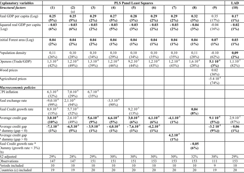
Table 1. Determinants of deforestation in Latin America (1948-2005)
Explanatory variables PLS Panel Least Squares LAD
Structural factors (1) (2) (a)
(3) (4) (5) (6) (7) (8) (9) (10) Real GDP per capita (Log) 0.25
(5%) 0.25 (5%) 0.29 (2%) 0.27 (5%) 0.28 (3%) 0.29 (2%) 0.29 (2%) 0.32 (3%) 0.35 (17%) 0.17 (1%) Squared real GDP per capita
(Log) - 0.03 (6%) - 0.03 (6%) - 0.03 (2%) - 0.03 (5%) - 0.03 (3%) - 0.03 (2%) - 0.03 (2%) - 0.04 (3%) -0.04 (16%) - 0.02 (1%) Initial Forest area (Log) 0.04
(2%) 0.04 (2%) 0.04 (2%) 0.04 (1%) 0.04 (1%) 0.04 (1%) 0.04 (1%) 0.04 (1%) 0.07 (1%) 0.03 (1%) Population density 0,11 (26%) 0,10 (28%) 0,10 (34%) 0,10 (29%) 0,10 (34%) 0,10 (35%) 0,10 (35%) 0,11 (28%) -0.10 (62%) 0,09 (2%) Openess (Trade/GDP) 1,3.10-4 (42%) 1,2.10-4 (49%) 1,3.10-4 (39%) 1,2.10-4 (46%) 9,2.10-3 (44%) 1,2.10-4 (43%) 1,2.10-4 (43%) 1,6.10-4 (28%) 5.1 10-4 (3%) 1,1.10-5 (82%) Wood prices 0.02 (36%) Agricultural prices -5.4 10-4 (74%) Macroeconomic policies CPI inflation 6,3.10-4 (32%) 7,0.10-4 (29%) 6,7.10-4 (35%) Real exchange rate
-9,0.10-8 (99%) 2,1.10-6 (94%) -3,5.10-6 (90%) Real Credit growth rate 8,9.10-3
(15%) 5,7.10-3 (52%) 9,2.10-3 (13%) 0,04 (8%) Average credit gap 3,0.10-4
(10%) 2,6.10-3 (49%) 5,6.10-5 (9%) 6,6.10-5 (5%) 3,0.10-4 (6%) 6,1.10-5 (6%) -4,1.10-3 (1%) 9.1 10-5 (5%)) 2,9.10-5 (87%) Average credit gap
* dummy (gap < 0) -7,1.10-3 (1%) -6,5.10-3 (5%) - 3,9.10-3 (1%) - 4,0.10-3 (1%) - 7,6.10-3 (1%) -4,2.10-3 (1%) -3.2 10-3 (9%)) - 0,06 (1%) Average credit gap
* dummy (gap > 0)
4,2.10-3 (1%) Real Credit growth rate *
Dummy (growth rate < 3%) (b) - 0,05 (6%) R2 adjusted 29% 28% 29% 30% 30% 30% 30% 32% 38% 29% Observations 147 147 151 151 151 153 153 153 111 153 Periods included 10 10 10 10 10 10 10 10 9 10 Countries (c) included 19 19 20 20 20 20 20 20 19 20
p-values in parenthesis, Coefficients significant at the 10% level in bold. t are robust to autocorrelation and heteroskedasticity. (a) Credit cycles are computed using a smoothing parameter equal to 150 instead of 100; (b) the use of a 5% threshold gives similar results; (c) when the real exchange rate is introduced, Guyana is dropped from estimations since the real exchange rate is not available.
4. 2. Structural variables
Regardless of the set of macroeconomic policies variables included, similar results are found on structural variables (table 1). First, the results suggest the existence of an Environmental Kuznets Curve: deforestation increases with the level of development when GDP per capita is smaller than 4160$, then decreases beyond this threshold. Second, the coefficient associated with the initial forest area is positive and statistically significant, thus showing a convergence phenomenon in the deforestation process. The estimated convergence parameter allows calculating that half the difference between actual and steady states values of forested area is squeezed in 17 years, other variables held constant. Third, population density and openness variables are both insignificant. As regards density, one could have expected a positive impact on deforestation in our sample since Central America countries exhibit both higher rates of deforestation and population growth (Bilsborrow and Carr, 2001). Given the strong inertia of demographic factors, the impact of density variations may be captured by country fixed-effects. Besides, Arcand et al. (2007) found similar results and suggest that the impact of these variables could operate through relative prices. Agricultural and forest products’ prices are only available from 1961 onwards, dropping about 40 observations from the sample. The variables are not significant (column 9 in table 1) since their effects may be caught by temporal fixed effects which allow controlling for common trends in international crop and forest products’ prices. Whether these structural variables are kept or not does not alter the results.20
4. 3. Macroeconomic policy
As regards the impact of macroeconomic policies, inflation, and the real exchange rate are both insignificant (column 1 in table 1). This result persists when macroeconomic policy variables are tested separately to reveal multicolinearity problems (columns 3 and 4). The lack of impact of real exchange rate variations is unexpected. It suggests that the driving force of deforestation is not the production of tradable goods in the sample. These variables are therefore dropped from the subsequent regressions (column 5 and following).
More interestingly, the coefficient associated with the credit gap is positive but weakly significant. When it is however multiplied with a dummy variable corresponding to a credit
20
Institutional quality is also taken into account since the Economic Freedom index from the Fraser Institute may be considered as a potential control variable. The time coverage only begins in 1970 and thus drops 3 of the 10 periods included in the sample. The non significant effect of this variable must be cautiously interpreted.
crunch, the estimated coefficient is negative and strongly significant. The marginal impact of negative credit gaps is given by the sum of the coefficients, and is negative (around – 0.005). By introducing a dummy corresponding to positive gap instead of a negative one, it is checked that this marginal impact is significant (column 7). This confirms the theoretical prediction of the second model, i.e. that credit crunches accelerate deforestation while credit booms do not. In others words, deforestation is driven by credit crunches episodes, but credit booms do not protect forests. This result is robust to the introduction of the real credit growth rate (columns 1, 2 and 5). The occurrence of a 14% credit crunch (1st quartile value) contributes to an additional 0.06% annual deforestation, which corresponds to 8% of total deforestation (column 6).21 This result enlightens that macroeconomic policies may have a significant short-term impact on deforestation dynamics.
The asymmetric impact of credit growth is unchanged if credit cycles are defined using a 3 or a 5 percent threshold (corresponding to the long run potential GDP growth) instead of the HP filter residual (column 8, and note (c)).
The Least Absolute Deviation (LAD) estimator (column 10) gives the median regression and hence provides results weakly sensitive to potential outliers. The standard errors are calculated with a non-parametric bootstrap method. Results are qualitatively similar to the Panel least Squares estimations: only credit crunches affect significantly deforestation.22
5. Conclusion
Economists have not been tempted to link deforestation and credit cycles in Latin American countries. This can be explained by the weak simple correlation between these two phenomenons. Peculiar characteristics of Latin American countries may however motivate further investigations since many Latin American countries are land abundant, exhibit rapid deforestation rates often experience macro instability that is often rooted in credit boom and crunches episodes. Recent available data show a coincidence between higher financial instability and deforestation increases. This paper provides a theoretical explanation and empirical investigations of this phenomenon. Econometric tests are conducted on the 1948-2005 period on an exhaustive sample of Latin American countries. The deforestation database is derived from a compilation of censuses carried out by the FAO. Moreover, various
21
Computed as the product of the marginal impact of credit crunches (0.005) multiplied by the mean value of credit crunches (0.08).
22
variables measuring credit cycles are calculated. The main output of the paper is to evidence the impact of credit cycles on deforestation. Precisely, it is shown that the deeper the credit cycles, the higher the deforestation rates. The results are robust to the introduction of usual control variables.
This paper confirms the role of short-term macroeconomic policies on deforestation and thus shows that the macroeconomic instability may have broader negative effects than that is usually acknowledged. It is not only detrimental to growth and welfare, but has also a negative effect on the environment through an increase in deforestation. Therefore the efficiency of usual instruments of environmental policies (taxation, norms and property rights) may be enhanced by macroeconomic policies aiming at downsizing credit cycles.
Statistical appendix
Table 2: Forest data sources (1948 -2005)
Survey Survey Year References Data
FOREST RESOURCES OF THE WORLD
1948 Unasylva, Revue internationale des forêts et des produits forestiers, Vol. 2(4), juillet-août, 1948
1948
WORLD FOREST INVENTORY
1958
FAO. 1960. World forest inventory 1958 - the third in the quinquennial series compiled by the Forestry and Forest Products Division of FAO. Rome.
1958
WORLD FOREST INVENTORY
1963 FAO. 1966. World forest inventory 1963, Rome
1963
FAO stat Various issues
FAO stat. CD-rom version 1998 (available between 1989 and 1994 on the FAO website
http://faostat.fao.org/site/418/DesktopDefault.aspx?PageID=418) 1968, 1973, 1978, 1983, 1988, 1993 FOREST RESOURCES ASSESSMENT – Interim report
1990 FAO 1993. Forest Resources Assessment 1990 - Tropical countries. FAO Forestry Paper No. 112. Rome.
1998 FOREST RESOURCES
ASSESSMENT – Interim report
1995 FAO. 1997, State of the World's Forests, Rome 1998
FOREST RESOURCES ASSESSMENT
2005
FAO. 2005, Global Forest Resources Assessment 2005: Progress towards sustainable forest management, FAO Forestry Paper 147, Rome
(or www.fao.org/forestry/site/fra2005/fr)
2005
Note: In order to keep a five-year frequency until the last period, 1998 is calculated by interpolating the forest cover between 1995 (or 1990, depending on availability and consistency of data) and 2000
Table 3. Average annual rates of deforestation in Latin American countries 1948 – 2005, percentages
48-57 58-63 64-68 69-73 74-78 79-83 84-88 89-93 94-98 99-05 Belize CA 1,51 0,28 0,13 0,70 0,74 0,00 0,00 0,00 0,00 0,00 0,34 Costa-Rica CA 3,79 2,52 2,88 3,37 4,20 0,61 -0,26 1,01 0,33 2,05 El Salvador CA 4,22 2,04 1,11 2,67 4,30 2,96 0,00 1,88 2,22 2,38 Guatemala CA 2,93 0,15 0,57 0,59 1,23 0,91 -2,13 -0,83 1,56 1,79 0,68 Honduras CA 2,72 0,00 0,00 0,00 0,00 0,00 0,00 3,71 4,32 1,19 Mexico CA -0,10 0,94 0,99 1,04 1,38 -0,75 -0,29 0,68 0,63 0,50 Nicaragua CA 0,70 1,84 2,03 2,26 2,50 2,80 2,33 1,44 1,71 1,96 Panama CA 3,11 0,65 0,67 0,69 1,71 2,65 0,79 0,19 0,13 1,18
Dominican Rep CAR 0,12 0,30 0,31 0,31 0,31 0,32 0,62 0,00 0,00 0,25
Haiti CAR 0,00 0,00 0,00 0,00 0,00 0,00 0,00 0,91 1,01 0,21
Jamaica CAR 11,26 0,48 0,49 0,50 0,51 0,53 0,21 0,16 0,16 1,59
Trinidad & Tobago CAR 2,60 0,51 0,41 0,42 0,43 0,43 0,44 -1,14 0,40 0,32 0,48
Bolivia SA 0,28 0,42 0,43 -0,19 0,00 0,00 0,00 0,59 0,63 0,24 Brazil SA 1,50 0,24 0,34 0,39 0,44 -1,11 -0,39 0,21 0,60 0,74 0,30 Colombia SA 0,37 3,39 0,15 0,68 0,36 0,00 0,18 0,56 -0,22 -0,03 0,54 Ecuador SA -3,64 1,27 1,23 0,19 0,00 0,00 -0,13 2,00 2,34 0,36 Guyana SA 0,01 -0,08 0,00 0,00 1,55 0,55 0,00 -0,16 0,11 0,04 0,20 Paraguay SA -0,52 0,23 0,24 0,24 1,93 4,46 2,98 0,23 0,88 1,19 Peru SA 1,38 0,00 0,00 0,00 0,00 0,00 0,01 0,17 0,19 0,19 Venezuela SA 3,32 0,77 0,81 0,84 -1,80 -3,19 -0,89 0,39 0,56 0,09 1,49 1,56 0,65 0,70 0,83 0,79 0,42 0,20 0,79 0,90 0,80
Source: Authors’ calculations from several issues of FAO censuses CA: Central American country, CAR: Carribean country, SA: South American Country
Table 4. Credit growth rate standard errors in Latin American countries 1948 – 2005 48-58 59-63 64-68 69-73 74-78 79-83 84-88 89-93 94-98 99-05 Belize CA 0,09 0,13 0,09 0,13 0,11 Costa-Rica CA 0,11 0,12 0,05 0,14 0,11 0,31 0,07 0,10 0,26 0,07 0,13 El Salvador CA 0,19 0,11 0,07 0,06 0,07 0,12 0,24 0,19 0,12 0,10 0,13 Guatemala CA 0,17 0,08 0,07 0,09 0,05 0,08 0,12 0,07 0,09 0,08 0,09 Honduras CA 0,25 0,10 0,11 0,11 0,05 0,06 0,05 0,13 0,10 0,12 0,11 Mexico CA 0,10 0,03 0,03 0,04 0,08 0,22 0,18 0,05 0,28 0,03 0,11 Nicaragua CA 0,08 0,25 0,51 1,88 0,11 0,03 0,48 Panama CA 0,12 0,11 0,07 0,04 0,10 0,06 0,10 0,13 0,07 0,08 0,09
Dominican Rep CAR 0,26 0,13 0,08 0,03 0,12 0,01 0,16 0,17 0,09 0,14 0,12
Haiti CAR 0,05 0,09 0,06 0,02 0,07 0,13 0,10 0,05 0,15 0,08
Jamaica CAR 0,35 0,12 0,12 0,14 0,17 0,10 0,28 0,17 0,32 0,20
Trinidad & Tobago CAR 0,38 0,08 0,08 1,18 1,33 0,10 0,07 0,15 0,07 0,38
Bolivia SA 0,42 0,04 0,05 0,09 0,31 0,49 1,25 0,14 0,13 0,05 0,30 Brazil SA 0,06 0,10 0,17 0,11 0,13 0,12 0,40 0,39 0,34 0,09 0,19 Colombia SA 0,12 0,14 0,08 0,04 0,10 0,13 0,10 0,15 0,08 0,04 0,10 Ecuador SA 0,11 0,10 0,08 0,11 0,06 0,22 0,13 0,67 0,19 0,23 0,19 Guyana SA 0,07 0,07 Paraguay SA 0,08 0,09 0,04 0,10 0,13 0,06 0,34 0,06 0,15 0,12 Peru SA 0,06 0,02 0,09 0,09 0,08 0,21 0,24 0,32 0,27 0,10 0,15 Venezuela SA 0,49 0,16 0,07 0,06 0,15 0,07 0,10 0,21 0,23 0,22 0,18 0,190 0,122 0,082 0,078 0,164 0,225 0,218 0,291 0,152 0,113 0,16
Source: Authors’ calculations from IFS.
Figure 1. Annual growth rates country averages of real credit (five-year moving average in bold)
-0,15 -0,1 -0,05 0 0,05 0,1 0,15 0,2 0,25 0,3 0,35 1 9 4 9 1 9 5 2 1 9 5 5 1 9 5 8 1 9 6 1 1 9 6 4 1 9 6 7 1 9 7 0 1 9 7 3 1 9 7 6 1 9 7 9 1 9 8 2 1 9 8 5 1 9 8 8 1 9 9 1 1 9 9 4 1 9 9 7 2 0 0 0 2 0 0 3
Mathematical appendix
* The Hessian matrix evaluated at the maximum in the first model (modern and subsistence sectors’ expansions) is the following:
− − − − + ≡ π * * * * * * * * * * * * * * 2 0 0 0 0 HH HK HL HH HL KH KK KL LH LH LK LL LL pF pF pF G G pF pF pF pF G pF pF G D
The sufficient second order condition for a maximum implies that the Hessian must be negative definite. That means in particular that D2π* >0. The optimal choice functions are implicit functions of the parameters and especially of r. The comparative static exercise on r allows simulating credit crunch (boom) when dr is positive (negative). When totally differentiating the first order conditions, the system of equations of four unknowns is the following: = − − − − + 0 0 1 0 0 0 0 0 * * * * * * * * * * * * * dr dH dr dH dr dK dr dL pF pF pF G G pF pF pF pF G pF pF G F G G HH HK HL HH HL KH KK KL LH LH LK LL LL
The Cramer’s rule allows deriving the optimal responses to changes dr (stars omitted) taking into account the sign of the Hessian and the hypotheses on the production functions:
(
TT HH LK HH TK LH)
G F F G p F F G p sign dr dLsign =− − 2 + 2 which is positive
(
HL HK LH HL LK HH)
G F F G p F F G p sign dr dHsign =− − 2 + 2 which is positive
(
)
(
)
(
)
(
2 2 2)
HL HH HH HL HH HH LL LL pF G pF G pF p G F G sign dr dKsign = + − − which is ambiguous
(
)
(
)
(
HL HK HL LK HH LL LL HK HH)
F G pF pF G G F F p F G p sign dr dH sign = 2 + 2 − + which is ambiguous* The Hessian matrix evaluated at the maximum in the second model (subsistence sector’s expansion) is the following: − − + = π KK KL HH HL LK LH LL LL F p F p G G F p G F p G D ~ 0 ~ 0 ~ ~ ~ ~ ~ ~ ~ 2
The sufficient second order condition for a maximum implies that the Hessian must be negative definite. That means in particular that:
0 ~
2π <
D and
(
G~LL+ pF~LL)
G~HH −( )
G~LH 2 >0 which is the determinant of the second principal minor. Next differentiating totally the first order conditions delivers the following system of equations of three unknowns: = − − + 1 0 0 ~ ~ ~ ~ 0 ~ 0 ~ ~ ~ ~ ~ ~ dr K d dr H d dr L d F p F p G G F p G F p G G KK KL HH HL LK LH LL LLThe Cramer’s rule allows deriving the optimal responses to changes dr:
(
HH LK)
G F G p sign dr L d sign ~ ~ ~ − − = which is positive(
HL LK)
G F G p sign dr H d sign ~ ~ ~ − − = which is positive(
)
( )
(
~ ~ ~ ~ 2)
~ LH HH LL LL pF G G G sign dr K dReferences
Amado, AM., MF. Da Cuhna Resende & FG. Jayme Jr, 2006 “Economic Growth Cycles in Latin America and Developing Countries” Text para discussão #297, December. Available on line:
http://www.cedeplar.ufmg.br/pesquisas/td/TD%20297.pdf
Anderson, A. 1990 “Smokestacks in the Rainforest: Industrial Development and Deforestation in the Amazon Basin” World Development, vol. 18, n° 9, pp. 1191-1205.
Angelsen, A. 1999 “Agricultural Expansion and Deforestation: modelling the Impact of Population, Market Forces and Property Rights” Journal of Development Economics, vol. 58, n° 1, pp. 185-218.
Arcand, JL., P. Guillaumont & S. Guillaumont Jeanneney, 2007 “Deforestation and the real exchange rate” The Journal of Development Economics, forthcoming
Barajas, A. & R. Steiner, 2002 “Credit Stagnation in Latin America” IMF Working Paper, March, 02/53. Mimeo, available on line: http://www.imf.org/External/Pubs/FT/staffp/2001/00-00/pdf/abrs.pdf
Barajas, A., R. Chami & T. Cosimano, 2004 “Did the Basel Accord cause a Credit Slowdown in Latin America?” Economia, Fall, pp. 135-182.
Barbier, EB. & JC. Burgess, 2001 “The Economics of Tropical Deforestation.” Journal of Economic Surveys vol. 15, n° 3, pp. 413-432.
Barbier, EB. & M. Rauscher, 1994 “Trade, Tropical Deforestation and Policy Interventions” Environment and Resource Economics, vol. 4, n° 1, February, pp. 75-90.
Barbier, EB. 2004a “Agricultural Expansion, Resource Booms and Growth in Latin America: Implications for Long-run Economic Development” World Development, vol. 32, n° 1, pp. 137-157.
Barbier, EB. 2004b “Explaining Agricultural Land Expansion and Deforestation in Developing Countries” American Journal of Agricultural Economics, vol. 86, n° 5, pp. 1347-1353.
Bernanke, B. and M. Gertler, 1989 “Agency Costs, Net Worth, and Business Fluctuations” The American Economic Review, vol. 79, n° 1, March, pp. 14-31.
Bilsborrow, RE. & DL. Carr, DL. 2001 “Population and land use/cover change: A regional comparison between Central America and South America” Journal of Geography Education, vol. 43, pp. 7–16.
Boucher, S., BL. Barham & MR. Carter 2005 “The Impact of Market-Friendly Reforms on Credit and Land Markets in Honduras and Nicaragua” World Development, vol. 33, n° 1, pp. 107–128.
Braun, M. & R. Haussmann, 2002 “Financial Development and Credit Crunches: Latin America and the World” In Latin American Competitiveness Report 2001-2002, J. Vial and P. K. Cornelius (editors), Oxford University Press.
Bulte, EH., R. Damania & R. López, 2007 “On the gains of committing to inefficiency: Corruption, deforestation and low land productivity in Latin America” Journal of Environmental Economics and Management, vol. 54, Issue 3, pp. 277-295.
Caballero, RJ. 2000 “Macroeconomic volatility in Latin America: A Conceptual Framework and Three Case Studies” Economia, Fall, pp. 31-107
Carr, DL., A. Barbieri, WK. Pan & H. Iranavi 2006 “Agricultural change and limits to deforestation in Central America” In Brouwer, F. & B. A. McCarl (Eds.) Agriculture and climate beyond 2015: A new perspective on future land use patterns, pp. 91–108. Springer.
Caviglia-Harris, J. 2003 “Sustainable Agricultural Practices in Rondônia, Brazil: Do Local Farmer Organizations Affect Adoption Rates?” Economic Development and Cultural Change, vol. 52, n° 1, pp. 23-50.
Chomitz, KM. & DA. Gray, 1998 “Roads, Land Use, and Deforestation: A Spatial Model Applied to Belize” The World Bank Economic Review, vol. 10, n° 3, pp. 487-512.
Chomitz, KM. & K. Kumari, 1998 “The Domestic Benefits of Tropical Forests: A Critical Review” The World Bank Economic Review, vol. 13, n° 1, pp. 13-35.
Cropper, M. & C. Griffiths, 1994, “The Interaction of Population Growth and Environmental Quality” The American Economic Review, vol. 84, n° 2, Papers and Proceedings of the Hundred and Sixth Annual Meeting of the American Economic Association, May, pp. 250-254.
Culas, RJ. 2003 “Impact of Credit Policy on Agricultural Expansion and Deforestation” Tropical Agricultural Research, vol. 15, pp. 276–287.
Culas, RJ. 2006 “Debt and deforestation” Journal of Developing Societies, vol. 22, n° 4, pp. 347-358.
de Camino, R., O. Segura, LG. Arias & I. Pérez 2000 Costa Rica Forest Strategy and Evolution of Land Use, World Bank Publications
Deacon, RT. 1999 “Deforestation and Ownership: Evidence from Historical Accounts and Contemporary Data” Land Economics, vol. 75, n° 3, pp. 341-359.
Dorner, P. & R. Quiros, 1973, “Institutional Dualism in Central America’s Agricultural Development” Journal of Latin American Studies, vol. 5, n° 2, November, pp. 217-232.
Edwards, S. 1995 Crisis and Reform in Latin America. From Despair to Hope, Oxford University Press
Eichengreen, B., R. Hausman & U. Panizza, 2003 Chapter in Other People’s Money: Debt Denomination and Financial Instability in Emerging Market Economies, B. Eichengreen and R. Hausmann (editors), University of Chicago Press. Traduction française: 2003, “Le péché original, le calvaire et le chemin de la rédemption” L’Actualité économique, Revue d’analyse économique, vol. 79, n°4, décembre, pp. 419-455
Eichengreen, B., R. Hausmann and U. Panizza, 2003 “The Pain of Original Sin” Mimeo. Available on line:
http://www.econ.berkeley.edu/~eichengr/research/ospainaug21-03.pdf
FAO, 2007 State of the World’s Forests. Available on line:
http://www.fao.org/docrep/009/a0773e/a0773e00.htm
FAO, 2006 FAOSTAT Archives Trade indices. Available on line: http://faostat.fao.org/site/416/default.aspx
Ferraz, C. 2001 “Explaining Agriculture Expansion and Deforestation: Evidence from the Brazilian Amazon – 1980/98” IPEA working paper #828, October. Available on line:
http://www.ipea.gov.br/pub/td/td_2001/td_0828.pdf
Fujisaka, Sam, W. Bell, N. Thomas, L. Hurtado, & E. Crawford 1995 “Slash-and-burn agriculture, conversion to pasture, and deforestation in two Brazilian Amazon colonies” Agriculture, Ecosystems and Environment, vol. 59, Issues 1-2, pp. 115-130.
Geist, HJ. & EF. Lambin, 2002 “Proximate Causes and Underlying Driving Forces of Tropical Deforestation” BioScience, vol. 52, n° 2, February, pp. 153-150
Gourinchas, PO., R. Valdés & O. Landerretche, 2001 “Lending Booms: Latin America and the World” Economia, Spring, pp. 47-99.
Gullison, RE. & EC. Losos, 1993 “The Role of Foreign Debt in Deforestation in Latin America” Conservation Biology, vol. 7, n° 1, march, pp. 140-147
Hecht, SB., S. Kandel, I. Gomes, N. Cuellar & H. Rosa, 2006 “Globalization, Forest Resurgence, and Environmental Politics in El Salvador” World Development, vol. 34, n° 2, February, pp. 308-323.
Horowitz, AW. 1996, “Wage-Homestead Tenancies: Technological Dualism and Tenant Household Size” Land Economics, vol. 72, n° 3, August, pp. 370-380
http://www.petersoninstitute.org/publications/chapters_preview/373/1iie3608.pdf
Kahn, JR. & JA. McDonald, 1994 “Third-world debt and tropical deforestation” Ecological Economics, vol. 12, n° 2, February, pp. 107-123
Kaimowitz, D. & A. Angelsen, 1998 Economic Models of Tropical Deforestation, CIFOR
Koop, G. & Tole, L., 2001 “Deforestation, Distribution and Development” Global Environmental Change, vol. 11, n°3, pp. 193-202
Mas, I. 1995 “Policy-Induced Disincentives to Financial Sector Development: Selected Examples from Latin America in the 1980s” Journal of Latin American Studies, vol. 27, n° 3, October, pp. 683-706.
Metzger, JP. 2003 “Effects of slash-and-burn fallow periods on landscape structure” Environmental Conservation, vol. 30, n° 4, pp. 325-333
Meyer, AL., GC. van Kooten & S. Wang, 2003 “Institutional, Social and Economic Roots of Deforestation: Further Evidence of an Environmental Kuznets Relation?” International Forestry Review, vol. 5, n° 1, March, pp. 29-37.
Myers, N. 1993 “Tropical forests: The main deforestation fronts” Environmental Conservation, vol. 20, n° 1, pp. 9-16.
Pacheco, P. 2006 “Agricultural expansion and deforestation in lowland Bolivia: the import substitution versus the structural adjustment model” Land Use Policy, Vol. 23, Issue 3, July 2006, pp. 205-225.
Randall, L. 1997 The Political Economy of Latin America in the Postwar Period, University of Texas Press Schultz, TW. 1964 Transforming Traditional Agriculture, Yale University Press.
Southgate, D., & CF. Runge, 1990 “The institutional origins of deforestation in Latin America” University of Minnesota, Department of Agriculture and Applied Economcis, Staff Paper n° P90-5.
Southgate, D., Sanders, J., & Ehui, S., 1990 “Resource Degradation in Africa and Latin America: Population Pressure, Policies and Property Arrangements” American Journal of Agricultural Economics, vol. 72, n°5, Proceedings Issue, pp. 1259-1263
Stiglitz, JE. & A. Weiss, 1981 “Credit Rationing in Markets with Imperfect Information” The American Economic Review, vol. 71, n° 3, June, pp. 393-410.
Thorp, R. 1998 Progress, Poverty and Exclusion. An Economic History of Latin America in the 20th century, Inter American Development Bank.
Tinker, PB., J. Ingram & S. Struwe, 1996 “Effects of slash-and-burn agriculture and deforestation on climate change” Agriculture, Ecosystems & Environment, vol. 58, June, pp. 13-22.