Flexibility of dynamic blending with alternative routings combined with safety stocks: case study in a mining supply chain

lamsade

LAMSADE

Laboratoire d’Analyse et Modélisation de Systèmes pour

l’Aide à la Décision

UMR 7243

Février 2020

Flexibility of dynamic blending with alternative

routings combined with safety stocks:

A.Azzamouri, M.Bamoumen, H.Hilali, V.Hovelaque

CAHIER DU

392

case study in a mining supply chain

Flexibility of dynamic blending with alternative routings

combined with safety stocks: case study in a mining supply chain

Ahlam Azzamouri

a

_{, Mouna Bamoumen}

a,b

_{, Hajar Hilali}

a,b

_{, Vincent Hovelaque}

a,b

_,

Vincent Giard

a,c1

a _{EMINES - School of Industrial Management, Mohammed VI Polytechnic University, Ben Guerir, Morocco} b _{Univ Rennes, CNRS, CREM - UMR 6211, F-35000 Rennes, France}

c _{Paris-Dauphine, PSL Research University, 75016, Paris, France}

{Ahlam.Azzamouri, Mouna.Bamoumen, Hajar.Hilali, Vincent.Hovelaque, Vincent.Giard}@emines.um6p.ma [email protected], [email protected]

Abstract - The blending problem has been dealt with in the literature since 1945 in

different industrial fields with the general aim of defining the optimal mixture to satisfy the demand under very specific constraints. Our paper proposes an extended version of the traditional LP formulation of the blending problem within the phosphate mining industry. This new “dynamic blending” method takes into account the slight instability of the chemical composition of source ores (SO), the availability of SOs in the mine and in secondary stocks (near the blending plants), storage constraints, the availability of blending processors and the orders to be met. The risk related to an unforeseen order of end-customers is mitigated by proper sizing of safety stocks for some critical SOs combined with the flexibility provided by dynamic blending. This model makes it possible to define the optimal quantities to be withdrawn from each source layer as well as the feeding transfers from the primary stock (mine) to the secondary stock. Dynamic blending allows an upgrade from a fixed-BOM rationale to a dynamic-BOM rationale in relation to SO availability and orders to be met.

Keywords:Dynamic blending, mine, alternative routings, safety stock, risk management

1_{ORCID: Ahlam Azzamouri: 0000-0001-6360-2162 ; Mouna Bamoumen: 0000-0002-9289-9476; Hajar Hilali:}

1. Introduction

The blending problem was the first Linear Programming problem solved by Dantzig, in 1947, involving use of his new simplex method, to address the problem of determination of an adequate diet at the lowest cost (Dantzig, 1982). During the last seventy years, many industrial problems involving blending have cropped up, some of them in mining industries (see section 2). The one we address is broader: it links blending with other upstream and downstream problems in a phosphoric Supply Chain (SC).

The OCP Group is the largest Moroccan company and a key player in the international phosphate market. Its integrated SC links the different processes of ore extraction, ore blending, phosphoric acid and fertilizer production and export. It comprises three independent axes: the north, center and southern axes. This paper focuses on the Ben Guerir subset of the Center axis, that includes a mine, from which 14 ores with different chemical characteristics are extracted and used as inputs (called source ores, SOs) in a blending plant to produce 5 different blended ores (outputs called merchantable ores, MOs), whose chemical composition is constrained (as illustrated in Table 2). The extraction process can be viewed as a push system because SO accessibility geological constraints disconnect extraction planning from short-term MO demand.

After blending, some MOs are directly exported while others are processed in one of two washing plants, before being either transferred for exportation, or turned into acids and/or fertilizers for subsequent export. Due to limited stocks, MOs are mainly produced to order and the blending process may be considered as a pull system. Process operations in the washing plants involve changes in product chemical and physical aspects to improve their quality.

Figure 1. Center axis of the OCP Phosphate Supply Chain

The dynamic blending (DB) problem has ten original features, whose combination makes it unique among the listed blending problems. SOs are not purchased in the international market but extracted from open pit mines, which are characterized by stacks of different homogenous layers, that may contain enough phosphate ores (SOs) or not (waste). A given SO at a given location remains inaccessible until the upper layers are cleared. The mining extraction program, therefore, entails a more or less delayed access to layers located in different parts of the deposit. Thus, SO feeding is characterized by eight (a to h) specific features. As several blending routings may be used, features i and j must be taken into account. Lastly, in this SC, demand characteristics cause a particular risk management problem under uncertainty (feature

k).

• Feature a) Extraction planning, defined at a tactical level, leads to scheduling SO supply corresponding to pushed flows that may not be removed immediately (primary stocks, in Figure 1).

• Feature b) The blending area has a limited capacity for each secondary SO stocks and a global limited capacity for all secondary SO stocks (that may be lower than the sum of each limited capacity).

• Feature c) Two conveyors feed the secondary stocks from primary stocks located at a number of deposit locations.

• Feature d) Extraction planning, enforces the withdrawal of SOs located at particular deposit locations to allow access to lower layers, by a particular deadline.

• Feature e) Features a, b and d may lead to temporary storage of SOs in a dumping area of the mine, before eventual retrieval; these operations are costly and add no value. The possible creation of stocks in the dumping area is therefore penalized in the model (proposed in section 3) with a high conventional cost allocated to it, in order to avoid exploring solutions that lead to such creation.

• Feature f) Estimation of the chemical composition of a SO located at a particular zone in the deposit, is used to define extraction planning. Additional samples refine this information when extraction is about to start. The difference between the expected initial composition and that actually found is sometimes substantial enough to treat that ore as a new SO, which should be stored separately in the secondary stocks of the blending area, so as to ensure that blending is based on reliable information on SO composition.

• Feature g) All the blended MOs comply with the quality charter, two of them – named internal MOs – are used downstream to produce two different phosphoric acids. Two successive batches of an internal MO will comply with the quality charter although their composition may differ. This composition instability creates phosphoric acid production issues that call for possible significant adjustments that are costly. Steering of blending operations mainly aims to ensure the stability of internal MO batches composition. This involves obtaining component target values for those internal MOs, as specified by phosphoric plant managers. Blending cost does not depend on the MOs to be produced as SO production costs refer to previously made tactical decisions.

• Feature h). Since features f (increase SO variety in primary stocks) and g (minimize the composition deviance of internal MOs) naturally lead to increasing the variety and volume of secondary stocks, this must be contained.

• Feature i) Some MO can be produced on the basis of two different routings: (1) Routing 1. dry blending where MO is shipped and sold as it is; (2) Routing 2. dry blending followed by a washing treatment including one to three additional processes: scrubbing, scrubbing + flotation and scrubbing + flotation + grinding. SO blending and processing time varies according to the selected routing.

• Feature j) Scheduling and routing choices for MO orders are assumed to be already defined on parallel blending plants and to match comply both with availability and operating time requirements.

The solution that was used up until just a few months ago was to select a blend of a required MO from some predetermined list of alternative Bills of Materials (BOMs), all of them being alternative blends. This solution has led to a preferential use of some SOs. According to the extraction schedule of an open pit, only a subset of SOs is accessible and none of the predefined blends may be used to process a MO order due to the lack of one of the SOs required by that BOM. This involves costly adjustments to ore extraction schedules in order to obtain the missing ores; in addition, this may increase dumping storage volume (feature e).

• Feature k) The schedule results from a pull process, triggered by the MO shipment program and derived, for internal MOs, by the acid production planning, itself pulled by a shipment program. On average, 30 to 50 ships each transporting 16.000 tons to 24.000 tons of acid are exported annually. This volume corresponds to 5 to 9 days of MO production in the blending area. The other MO orders are also pulled by an ore shipment program in 20.000 tons or 50.000 tons ships, corresponding to 3 to 8 days of MO production. Sometimes, a

programmed shipment is advanced by one week or a decision is taken to satisfy an order for acid or ore on a spot market, which corresponds to an amount of dry blended MO that departs from the currently selected routing (see §4.2). These changes are not known until the very last moment; they cannot be defined in terms of probabilities and thus must be managed in uncertain environment. In this paper, the risk focused on needs to be addressed not only through dynamic blending but also by creating specific stocks. These stocks concern SOs in secondary stock and are referred to as “security stocks”, to establish the distinction with those safety stocks that are used in stochastic universe.

In order to address this complex problem defined by features a to k, we propose in this paper: i) a dynamic optimization model that defines jointly SO feedings from the mine and optimal blends of MO orders to meet, avoiding the issues created by fixed BOMs; ii) a mitigation of the risk of change in demand order downstream, by setting aside specific security stocks defined in uncertain universe.

In section 2, we present our analysis of the literature. Our proposed blending model and risk management approach are described in Section 3. Section 4 illustrates the flexibility delivered by the blending model and the improvement of risk control achieved by combining dynamic blending and security stocks. After a short description of the implementation of the DB model (Section 5), we end with a conclusion (Section 6).

2 Literature review

In this section, a concise review of the literature on blending problems is provided along with a summary of the relevant research on sizing security stocks under uncertainty.

2.1 Blending literature

recipe respecting some composition constraints, with the main aim of minimizing cost. The first study addressing the blending problem was Stigler’s (1939) work on the adequacy of diets at various income levels (Dantzig 1982). In 1947, Dantzig found a numerical solution to the problem using linear programming. In the 70’s and 80’s, many authors used linear programming (LP) models to approach blending problems in different industries including agrifood, chemical oil, cement, flour milling and mining. An analysis of existing literature shows that blending problems as specified by the 11 features described in our introduction, has yet to be studied (see Table 1). We believe that all main analysis criteria refer to these features, which fall into three themes:

Table 1. Article analysis grid

Q ua ntity Qu al ity Q ua ntity Qu al ity Q ua ntity Qu al ity Q ua ntity Qu al ity 1 Mustafa Kumral 2003 X X X IL X X X Chance-Constrained Programming, Multi-objective simulated annealing X X

2 Ralph Steuer 1984 X X X IR L X X O X Multiple objective linear _programming X

3 Chanda and _Dagdelen 1995 X X X IL R P X X R S M X

Goal programming and interactive graphics

systems X X

4 Ashayeri et al. 1994 X X X IR P X X O X Mixed-integer _programming X X X

5 Karmarkar and _Rajaram 2001 X X X IR S L X X IR S L O X Mixed integer nonlinear _programming X X 6 Bilgen and _Ozkarahan 2007 X X X IR S L X X IR S L O X Mixed integer linear _programming X X 7 Williams and _Haley 1959 X X X R P P X X O Linear programming X

8 Oddsdottir et al. 2013 X X X IR P L P X X IR O M Mixed integer nonlinear _programming X X

9 Bengtsson et al. 2013 X X X L IR P L P X X IR O S X Robust solution approach _(Heuristic) X X

10 Yoon et al. 1997 X X X L S X S X X Linear programming X X

11Jonuzaj and _Adjiman 2017 X IL S X X R M X Generalized Disjunctive _Programming X X X

12Kural and _Özsoy 2004 X X IL S S X S S S X Linear multivariable _{stochastic model} X X

13 Montante et al. 2016 X X X IR P X X IR X X

Numerical calculation of chemical equations and Computational Fluid Dynamics (CFD) simulations

X X X

14 Stokes and Tozer 2006 X X X IR X X IR O Non linear programming X X X

15 Goldsmith 1966 X X X R S L S X R S M X Statistical approach X X

16 Cain and Price 1986 X X X IL IR S X X IR S X Probabilistic programming X X

Us Azzamouri et al. 2019 X X X L IR S L P X X IR S L O S X Mixed integer linear _programming X X X X Legend:

* Availibility: L: Limited. IL: Illimited. * Stocks capacity: L: Limited. IL: Illimited * Blending plants: P: Parallel. S:Single

* Inputs/outputs supply type: R: Regular. IR: Irregular. P: Parallel. S: Sequential * Blending context: S: to Stock. O: to Order. S: Single-stage. M: Multi-stage. Blending area supply O ut put s st oc ks ca paci ty S/ O A rtic le N um be r A ut hor s Y ear

Industry type Input

B le ndi ng pl ant s In pu ts s to ck s cap aci ty C as e st udy M ini ng Food indus tr y C he m ic al indus tr y O il indus tr y C em ent indus tr y M ill indus tr y characteristics Inputs over time A va ilib ility Supply type

Output Blending _context Approach _type

Resolution method Resolution criterion Ot he r Fix Variable R/ IR _P/S Fix Variable R/ IR _P/S S/ M Ot he r D et erm in is tic St oc ha st ic Co st Q ua lity Outputs characteritics over time

• Input supply. There are two types of supply processes : i) Blending units are supplied by simple conveyors, which requires a sequential (successive) supply of inputs; this is illustrated by the case of bulk grain mixture (Bilgen and Ozkarahan 2007), the semi-continuous mixture of materials (Goldsmith 1966), and the raw material mixture to produce cement flour (Kural and Özsoy 2004); ii) the parallel supply of inputs is used in the mixture of fertilizers (Ashayeri et al. 1994), of crude oils (Bengtsson et al. 2013; Oddsdottir et al. 2013), of sausages (Steuer 1984), of coking coal (Williams and Haley 1959) and of ores (Zhang et al. 2011).

• Productive context. This defines whether the blending is carried out under a rationale of:

i) pull flow, which means that mixing is done to meet a specific need expressed by an

internal or external customer (make-to-order). This case is illustrated by Bengtsson et al. (2013), Bilgen and Ozkarahan (2007), Chanda and Dagdelen (1995), Karmarkar and Rajaram (2001), Oddsdottir et al. (2013), Steuer (1984), Stokes and Tozer (2006), Williams and Haley (1959) and Zhang et al. (2011); ii) a push flow of make-to-stock pending potential demand, as is the case with Ashayeri et al. (1994) and Kural and Özsoy (2004). • Optimization criterion. Most articles refer to an economic optimization criterion, such as

i) the minimization of costs, whether it be production costs as illustrated by Ashayeri et al.

(1994), Cain and Price (1986), Kumral (2003), Yoon et al. (1997) and Zhang et al. (2011) or transportation costs (Bilgen and Ozkarahan 2007); ii) the maximization of profit as in the case of Bengtsson et al. (2013) and Oddsdottir et al. (2013); iii) other articles focus on mixture quality (Montante et al. 2016; Jonuzaj and Adjiman 2017). While others combine multiple criteria, a) of cost and quality (Karmarkar and Rajaram 2001; Stokes and Tozer 2006) or b) of cost, quality and profit (Steuer 1984). Moreover, the minimization of the penalties generated by deviations from the target values is also a criterion of resolution

addressed in some articles (Chanda and Dagdelen 1995; Goldsmith 1966; Kural and Özsoy 2004).

Based on our analysis, we were able to confirm that our work addresses a specific blending problem combining several characteristics not previously taken into account in research work: i) inputs extracted upstream of the integrated supply chain have variable characteristics over time (feature f); ii) variation in the availability of inputs due to layer accessibility over time (features a and d); iii) the sequential supply of input stocks with limited storage and transport capacity (features b and c); iv) outputs may be manufactured according to different routings which potentially modify chemical composition of inputs (feature i). These constraints must be taken into account to meet demand in terms of quality and quantity. In addition, our work tackles the problem of stabilizing the chemical composition of the batches sent to the phosphoric acid plants in the interests of global SC performance improvement. In that respect, the variation and uncertainty of the system’s characteristics determine the specific nature of the problem at hand.

2.2 Mitigation of uncertainty in literature

Modern history of uncertainty was built in the early 20’s by Economics Philosophy introduced by Knight (1921) and Keynes (1936). Several research communities (economists, decision-makers, risk analysts, behavioral scientists) proposed different taxonomies of uncertainty (Naji 2016), which overlap to a great extent (Smithson 1989; Klir and Wierman 1999; Oberkampf et

al. 2004; Ayyub and Klir 2006; and Wierman 2010). There emerges three axes of analysis:

• Stochastic uncertainty, defined as an inherent variation associated with the physical system or the environment (Oberkampf et al. 2004), some of whose parameters can be described by probability distribution (Walker et al. 2003). In this context, operational research proposed several stochastic models for some sub-system operations (supply for example),

which provide analytical solutions, while optimizing a criterion defined by some mathematical expectations. In some complex cases, this approach is not workable and the modelling is performed on a spreadsheet where parameter values are replaced by the occurrence of a random variable. The use of the Monte Carlo approach provides empirical probability distributions for some indicators, which channels the determination of order variables acting on relevant system operations.

• Ambiguity, which relates to the multiplicity of alternatives without preference to any alternative (Wierman 2010) or the possibility to describe their probability distribution (Walker et al. 2003). Rockafellar and Wets (1991) considered the scenario model as a common approach to model uncertainty in practice. Kouvelis and Yu (1997) claimed that the scenario model is one of the important tools in structuring data uncertainty when multiple future alternatives are potentially realizable without any attached probabilities. • Vagueness, which refers to poorly defined or indistinct information (Oberkampf et al. 2004)

and describes the inability to develop scenario representation (Walker et al. 2003). Interval representation is widely used in practice to represent this type of uncertainty (Ben-Tal and Nemirovski 2000; Lin et al. 2004). This model is useful when only the upper and lower bounds can be determined with certainty and the decision-maker is not able to choose specific scenarios. The polyhedral sets-based representations also represent a useful tool to model uncertainty. The geometry of the convex set leads to different uncertainty sets such as box sets, ellipsoidal sets, polyhedral sets, etc. (Ben-Tal et al. 2009).

The uncertainty addressed in this article concerns the possible occurrence of an unexpected order (change in demand). The description of a few plausible scenarios is possible, without it being possible to define the probability of their occurrence, owing to the great variety of contexts in which such events occurred in the past. This uncertainty clearly belongs to the ambiguity type.

Lastly, we note that three complementary approaches dealing with uncertainty (Bamoumen et al. 2018): i) improve the quality of factual and procedural information used in decision-making; ii) oversize productive resources to increase system reactivity and flexibility;

iii) create stocks of finished or intermediate products along the supply chain. Our proposed

approach combines two of these risk management measures, namely adoption of the dynamic blending model, which is of the procedure improvement type, and building security stocks of intermediate products rather than finished ones, for reasons of efficiency. These security levels are to be defined in uncertain universe. Yet the uncertainty, as defined in our case, prevents designing security stocks analytically (a traditional solution in the context of stochastic uncertainty), but in a very specific manner.

3 Dynamic Blending Problem Formulation

In section 3.1, to facilitate understanding of our model, we simplify the blending problem by assuming that all the outputs (MOs) are produced using routing 1 (dry blending), and we go on to generalizing our model by introducing the possibility of alternative routings (section 3.2). As these models are implemented with an optimization software based on Algebraic Modelling Language (AML) (Kuip 1993), some relations (e.g. relation 4) use predicates to restrain the used domain of some indexes.

3.1. Dynamic Blending Problem Formulation using the dry blending routing for all output orders

Indexes

j Output index(j1,...,J). Output is merchantable ore obtained by blending. The subset E of the set of outputs concerns outputs directly used downstream to produce acid phosphoric (feature g).

i Input index ( 1,...,I)i . Input is extracted ore (in primary or secondary stock).

c Component index (c1,...,C).

t Period index ( 1,...,T)t , in day in this paper.

k Order index (k1...K). Order k relates to a single output.

λ_k Index of output =λj _kto be produced for the kth _{order (that relates to a single output).}

Parameters

α_ci Percentage of the weight of component c in the total weight of input i. D_k Quantity (in ton) of output λ_kto be produced for order k.

Min

β_cj Minimal percentage of the weight of component c in the total weight of output j.

Max

β_cj Maximal percentage of the weight of component c in the total weight of output j. δ_kt Boolean parameter meaning order k is processed during periods t if δ_kt  (otherwise 1

δ_kt  ) 0

ν_k Production time of order k (ν_k



_tδ )_kt .

ρ Transfer rate of a conveyor. A given input i cannot be transported, during period t, by more than one conveyor, all conveyors having the same transfer rate.

0

S_i Initial stock (in ton) of input i in the blending zone secondary stock; used in the recurrent relation (3).

R_t Number of conveyors available during period t, (feature c).

B_it Free cumulative availability (in ton) of input i at the end of period t in the primary stock, regardless of withdrawals of input i, from initial stockB_i0, (feature a).

c

B_it Constrained cumulative availability (in ton) of input i at the end of period t in the primary stock (feature d). See illustration in Figure 3.

Min

S_i Desired security stock (in ton) of input i at the end of any period t.

Max

S_i Maximal stock (in ton) of input i at the end of any period t in the secondary stock (feature

b).

Max

S Maximal used storage (in ton) at the end of any period t in the secondary stock (feature

b).

θ_i Penalty cost for a unit of input i at the end of period t in the secondary stock, when its level is under the desired security stock.

Max

K Limit number of the different inputs stored in the secondary stock at the end of the planning horizon T (feature h).

κ Penalty cost for a unit of input i sent in the dumping area, when the part of the secondary stock devoted to input i is full (feature e).

M High value; one can choose M=SMax.

τ_cj Target percentage of the weight of component c in the total weight of output j.

Variables

ik

x Quantity (in ton) of input i used in the production of order k that relates to output =λj _k. 

It is assumed that the consumption of all inputs used to produce a given order k is linear over its production time. Thus, input i consumption by order k during period t is equal to

/ ν

ik k

x , if δ_kt  , and 0 otherwise. 1

it

y Binary decision variable y_it  if feeding of input i in the secondary stock of the blending 1 zone, from the primary stock, occurs during period t (and 0, otherwise).

Existence of the decision variable y is subject to free cumulative availability_it B_it. As a given input i cannot be transported, during period t, by more than one conveyor, the quantity of input i to be conveyed to the blending zone is ρy_it.

it

S Stock (in ton) of input i in the secondary stock at the end of period t. It is a linear combination of decision variables.

it

w Missing quantity (in ton) of input i in the secondary stock at the end of period t when its level is under the desired security stock.

it

z Quantity (in ton) of input i sent to the dumping storage at the end of period t, because it cannot be stored in the secondary stock due to the lack of space (feature e).

i

u Binary variable which is equal to 1 if input i is still present in the secondary stock S_iT 0 at the end of the planning horizon T, and null otherwise (feature f)

  Absolute gap between the required weight of component c in the quantity of _ck output λ_kto be produced for order k, and the obtained weight obtained by the optimal blend of inputs.

To illustrate the predicate notations, the expression _|

k

k



_E refers to the sum for all

1,...,K k , subject to _kE . Problem definition | Min( θ κ σ . ) k i it it c ck i w   t iz  k c 



 



E



(1) Subject to D , ik k ix  k



₍₂₎ Min Max β_ck 



_iα_ci(x_ik / D ) β_k  _ck ,  c k, (3) , , 1 ρ _{| kt 1} / ν , , 1 i t i t it _k ik k S S _  y 



_{ } x   i t (4)

0, , it S   i t ₍₅₎ | Bit 0 it R ,t i  y  t



₍₆₎ B_it  ρ



_{t t} y_it, , i t ₍₇₎ c B_it  ρ



_{t t} y_itB , ,_it  i t ₍₈₎ Max S , it iS  t



₍₉₎ Min 0, , , , it it i it w i t w S S i t      (10) Max 0, , S , , it it it i z i t z S i t      (11) T Max M , K , i i i i S u i u i     



(12) α τ D τ D α k k ck _i ci ik c k ck c k _i ci ik x x            





c,k|kE (13) Comments

• The scheduling of production orders is assumed to be already established and consistent with blending processors availability (→ processors are ignored in our formulation) (feature

j). In our case study, every week, the plant manager receives a 4-weeks order book, that

constitutes a set of K sequenced orders to satisfy; only the first order is frozen in this rolling planning.

• Relation (2). Flow conservation constraint that links inputs used to produce the required quantity of an output. In a dry blending environment, there is no loss during dry blending. • Relation (3) represents the quality charter constraint (feature g), which adapts the classic

blending composition constraint (β_cjMin



_iα_ci(x_ij/ D ) β_j  _cjMax), considering that order k relates to output j_k.

• Relation (4) is a flow conservation constraint of the stock of input i in the blending zone secondary stock at the end of period t, where S depends on its previous level _it S_{i t, 1} , increased by supplies ρy_it during periods t t and decreased by the consumption of this input during periods t t.

• Relation (5) ensures that the stock of input i in the blending zone secondary stock is never depleted at the end of any period t.

• Relation (6) constraints input withdrawal process from primary stocks to secondary stocks by the number of conveyors available during period t.

• Relation (7) constraints input withdrawal process from primary stocks to secondary stocks by a sufficient available build-up (feature a).

• Relation (8) constraints input withdrawal process from primary stocks to secondary stocks by a sufficient withdrawal not to excess the constrained cumulative availability (feature d) • Relation (9) constraints overall storage to keep it below SMax (feature h).

• Relations (10) replace the hard constraint S_itSMin_i which may prevent from finding a

feasible solution of the problem at hand; they calculate the missing quantity w of input i _it

in the secondary stock at the end of period t, when its level is under the desired security stock.

• Relations (11) calculate the quantity of input i sent to the dumping storage at the end of period t due to the lack of space in the secondary stock (feature e).

• Relations (12) calculate and constraint the diversity of inputs at the end of the planning horizon T (feature h)

• Relation (1) is the objective function made of the sum of three costs: a cost of non-respect of security stock (



_iθ_iw_it), a dumping storage cost (κ

 

_{t i}z_it) and a deviance cost of outputs immediately used downstream to produce phosphoric acid ( _| σ . )

k c ck

k c 



E



. The used unit costs θ_i, κ and σ_c are fictitious and defined to drive the solution toward what may be considered as preferable (to avoid dumping, to privilege the composition stability of output used to produce acid and to keep a minimal protection against risk) • Figure 2 completes Figure 1 by mentioning the decision variables.

Figure 2. Blending Process (dry blending, before processing at the washing plant)

• Figure 3 provides a fictitious example of cumulative free and constrained availabilities of a given input and illustrates their possible impact on removal of this input from the primary stock.

Figure 3. Example of cumulative free and constrained availabilities. 3.2. Dynamic Blending Problem Formulation with Alternative Routings

According to feature i, the production of outputs may be obtained on the basis of one among several possible alternative routings. This leads to an extension of the model described in §3.2, where: i) no change occurs in variables, as the decision variables are independent of routing used; ii) demand D_k is still defined after the last process of the routing used; iii) the model concern still the dry blending process but with some parameter changes, when followed by an additional process in the washing plant; iv) only 3 relations of the previous model must be adapted.

Additional index

h Routing index (h1,...,H). Routing h1, is the dry blending routing, used for some merchantable ores to be directly exported. The others routing are performed in a washing plant and may (or not), be performed immediately after the first dry routing, depending

on plant configuration. Routings h1 (dry blending) and h2 (dry blending + scrubbing in a washing plant) are used in the Center axis.

Additional parameters

η_ih Reduction weight rate of input i (η_ih , when using routing 1) h1. To retain a general formulation, one defines η_i1 (dry blending process). 1

γ_cih Distortion rate the initial proportion α_ciof component c in input i , when using routing

1

h ; γ_cihcan be greater or lower than 1. To keep a general formulation, one defines

1

γ_ci   (dry blending process). 1, ,i c

μ_k Pre-defined routing number used by order k (feature j).

Adapted problem definition and constraints

_λ .η_μ D , k k i i k ix  k



(2’) βMin (α η_μ γ _μ ) / D βMax, , k k k k c 



_i ci i  ci xik k c  c k (3’) μ μ cλ cλ μ μ (α η γ ) τ D τ D (α η γ ) k k k k k k ck _i ci i ci ik k ck k _i ci i ci ik x x              





c ,k|kE (13’) Comments

• The decision variable x concerns the quantity of input i (in ton) used to produce order k _ik and is independent of routing μ_k.

• Relation (2’) replaces relation (2) which is a flow conservation constraints. When μ_k 1 (dry blending routing), η_i1 and relation (2’) becomes relation (2). One can remark that i) 1

when μ_k  , the quantity 1 _λ .(1 η_μ )

k k

i i

ix 



of inputs used to produce output _k is eliminated during the washing process; ii) The total quantity of inputs used to produce output j is not only greater than D_jh if h1, but also depends on the structure of inputs used, that is to say on the chosen blend.

• Relation (3’) replaces relation (3), considering the reduction weight rate of input i (η )_ih and the distortion rate (γ_cih) of the initial proportion α_ciof component c in input I, when using routing h. One must note that, if routing h1 is used, it is not possible to derive, from

Min Max

β_cj ;β_cj

 

 , the component ranges constraints of an output j before its entry into the

washing plant (and after the dry blending), because such bounds must be independent from the blending solution, which is impossible since the composition and the total weight of inputs used by routing h arise from the selected blending solution.

• Relations (13’) replace relations (13). The target of % value for component c in output j does not depend on the chosen routing but relations (13) must be adapted to consider the reduction weight rate of input i (η )_ih and the distortion rate (γ_cih) of the initial proportion

α_ci of component c in input i, when using routing h.

• With routing h1, the total quantity of inputs to be processed in the dry blending plant  and thus the production time ν_k depends on the blending recipe (see comment ii for relation (2’)). In the dry blending model, we have assumed that order k is processed during periods t such that δ_kt  , which leads to the production time 1 ν_k 



_tδ_kt and, implicitly, to the production rate D / ν_{k k}. If ν_k is not a parameter, relation (4) cannot be linear. Our formulation allows to address that issue, because the production rate may differ significantly from its nominal value. Thus, it suffices to define ν_k as “average” production time and to derive order schedule from it, the value of δ_kt, then serving as a problem parameter. Note

that if adjustment through production rate variations does not produce the expected result, then one will need to adjust the order schedule to avoid any overlapping or stoppage of production.

• Relations (1), (2’), (3’), (4) to (12) and (13’) define the generalized blending model. • A last important point concerns the washing routing which is a continuous process

performed in a large special tank which is not emptied between two successive production orders (POs). As a result, the optimal blend is not unrelated to the PO schedule, though the distortion may be insignificant. Taking data from Table 6, with a production rate of 800 T/H in the washing unit, a PO of 35,000 tons for a given MO that uses 45,000 tons of SOs, will be processed in 56 hours. Given, in addition, that the capacity of the tank is around 5,000 tons and contains about 10% of blended SOs at any moment, one must build into the definition of the optimal blend the use of an inevitable input of 500 tons corresponding to the material left by the preceding PO, whose composition is, of course, perfectly known. These considerations are ignored by the numerical examples presented in this article.

4. Illustration of the Dynamic Blending Approach

The data used are those of the Ben Guerir blending plant (Center axis of OCP’ SC). The blending process takes into account 5 components to characterize 14 inputs (SOs) and 5 outputs (MOs), among which the first two are internal MOs. For our purposes we only use 3 outputs to limit the size of the tables. We noted above that the characteristics of these inputs may vary slightly depending on the location of the extraction, and therefore over time; those selected for this case study are listed in Table 2 (which lists only the components that one pay attention to). It also shows the reduction rate η_i2 of input i after scrubbing in the washing plant (routing

2

h ) and, directly, the coefficient ω_ci2, to be used with that routing. The distortion rate γ_ci2

Table 2. Composition _ciof inputs, reduction factor η_i2and coefficient ω_ci2

Table 3. Quality charter

We study2 the flexibility of blending, first in a static mono-period context (§4.1) and then in a

dynamic context (§4.2), before illustrating the impact of the risk based on the principles of flexi-security stocks (§4.3).

2 _{All the examples referred to in §4.1, §4.2 and §4.3 have been solved using the software developed for OCP and used by the}

Center axis. The software encapsulates the parameterized generic model (described in section 3) formulated with FICO's Xpress-IVE AML (Algebraic Modeling Language), coupled with a data entry interface for problem feeding from a relational database, allowing the instantiation of an optimization problem to be solved.

i =1 C3 sup i =2 SA2 i =3 C3G i =4 C1 i =5 C0 i =6 C4 i =7 C5 i =8 C2 sup i =9 SB i =10 SX i =11 C3 inf i =12 C1 Exp i =13 C2 Exp i =14 C6 c =1 BPL 50.01 55.87 56.95 59.5 59.50 61.00 59.00 60.00 61.50 63.00 64.00 65.50 65.50 65.72 c =2 CO2 3.70 7.74 5.36 4.50 5.20 4.83 7.72 5.08 5.24 5.50 4.95 5.90 4.61 4.95 c =3 MgO 0.99 0.65 0.94 1.15 1.20 1.49 1.70 0.91 0.80 0.80 1.12 0.80 0.65 1.23 c =4 SiO2 24.00 8.00 17.19 9.50 8.50 11.74 9.79 11.50 8.00 11.00 10.00 7.50 8.00 6.00 c =5 Cd/B 7.00 16.00 6.00 11.00 8.00 10.00 14.00 12.00 10.00 10.00 5.00 12.00 13.00 9.00 0.88 0.84 0.85 0.87 0.9 0.81 0.74 0.87 0.83 0.77 0.92 0.95 0.9 0.89 c =1 47.83 51.90 52.23 57.25 59.22 54.54 48.46 53.76 56.50 53.70 64.82 72.80 65.55 65.33 c =2 2.80 5.85 4.60 3.56 4.35 3.63 3.37 4.37 3.17 3.09 4.73 5.15 4.10 4.22 c =3 0.64 0.45 0.56 0.81 0.88 0.69 0.61 0.60 0.49 0.46 0.87 0.47 0.48 0.70 c =4 18.48 5.62 11.25 8.17 7.56 8.91 5.49 8.68 5.98 7.63 8.05 6.00 6.06 4.22 c =5 5.77 8.70 4.11 6.82 5.13 4.50 4.56 9.00 7.66 7.11 4.31 9.76 10.08 6.67

Coefficient ic 2 of component c in input i with routing h =2

Composant

c

Share ci (%) of component c(<5) in the weight of input i

c=5 unit: ppm Input (SO) i

Component

c

Reduction factor i 2 from dry blending and washing plant

j =1 (h =2) Tess j =2 (h =2) Stand j =3 (h =1) MT c =1    c =2    c =3    c =4    c =5   

Constraints on the share cjh (%) of component c in the weight of output j Output (MO) j

Compo

n

ent

4.1 Blending Flexibility in a Static Context

In this context, the previous model formulation of section 3.1 must be adapted as the blending problem is set for a single period during which either a single order, that uses routing 1 or routing 2, is to be produced in a single blending plant (section 4.1.1) or 3 orders of 3 different outputs are to be produced in 3 parallel blending plants (section 4.1.2). Thus, x can be _ik

replaced by x_ij and _k disappears. Relation (2’) becomes



_ix_ij.η_ijD ,_j j and relation (3’) becomes β_cjMin



_i(α_ciη γ )_ij _cij x_ij/ D_jβ_cjMax,  c k, . Reference to time disappears, which leads to removing variables y , _it w et _it z and relations (4) to (13). The secondary stock is no _it

longer fed from the primary stock and blending is done using the initial secondary stock. Accordingly, constraint (5) becomes S_i0



_ix_ij,i. For our case study, we simplify the objective-function, as its definition does not change the performance in terms of flexibility, and choose to minimize consumption of component c1 in the production of D_j

1

(Min(



_ix_ijc ))_i . Other objective-functions could, as well, be chosen to illustrate blending flexibility, and to reach the same conclusions.

We will first look at the production of each of the 3 outputs separately (§4.1.1), and under (§4.1.2) will turn to simultaneous production of these outputs by as many blending units operating simultaneously.

4.1.1 Separate productions occurring simultaneously

Our aim is to determine successively and independently the optimal blend for output j, to meet demand D_j100 tons, defined after the washing plant for j1 and j2 produced with routing h2, and defined after the dry blending unit, for j3, produced with routing h1. To prevent any input shortage, initial stocks are oversized(S_0i100). The data in Table 2, Table 3 and Table 4 serve to confirm that for j2 (MO “standard”) after reduction achieved

by the processing of inputs (η )_i2 , the washing plant uses 131.18 tons of SOs to deliver

2

D 100 tons of MO “standard” ( 25.40 84% 92.98 74% 12.8 77%)      in compliance with the quality charter limits. Output composition that matches the quality charter depends on the inputs consumed and the selected blend



_iη_i2(x_ij/ D )_j .

Table 4. Unconstrained optimal solution for outputs 1 to 3 (in tons)

In order to be able to illustrate the huge variety of possible solutions, not generally perceived by scheduling managers, and facilitate the adoption of the dynamic blending approach, we forced the problem to use a number N of inputs (this parameter N taking successively all possible values), and also imposed a minimum quantity of the inputs used in the blend ( >ε D )x_ij  _j . The blends found for different values of N and ε 5% are reported in Table 4. It is obvious that if the optimal blend for output j uses N*_j inputs, with x_ij  ε D_j, we

find the optimal solution (Table 4) that becomes less performant once it moves away fromN*_j

.We can then note that when N>N*_j, N-N*_jinputs take valuex_ij=ε D _j, in order to limit

objective function degradation . Parameter ε , which must be ε 1/N , can prevent the use of all the inputs if it is relatively large but, if it is relatively small, for exampleε 1% , it enables finding a solution using all the inputs (e.g. for ε 1% and j1 we can produce it with N 13

inputs, with 6, 35, 41, 2 and 30 respectively for, i = 2, 3, 7, 11, and 14 and 1 for the other 8 inputs). The two studied MOs are internal MOs that use routing 2 (dry blending + washing),

i = 1 i = 2 i = 3 i = 7 i = 10 i = 12 i = 13 i = 14 j=1 (h =2) - 8.84 27.62 76.86 - 6.31 - 7.00 126.62 j = 1 65.43 5.00 0.75 8.50 6.50 j=2 (h =2) - 25.40 - 92.98 12.80 - - - 131.18 j = 2 65.12 5.02 0.75 7.51 7.37 j=3 (h =1) 7.02 5.52 - - - 7.47 25.69 54.30 100.00 j = 3 64.00 5.00 1.00 8.00 10.50 7.02 39.76 27.62 169.84 12.80 13.78 25.69 61.30 357.81 - 6.98 21.81 60.70 - 4.98 - 5.53 100% - 19.36 - 70.88 9.76 - - - 100% Components j=1 (h =2) j=2 (h =2) c =3 MgO c =4 SiO2 c =5 Cd/B Ou tp ut j  % xij i xij cjh _BPLc =1 _COc =2₂ Input (SO) i / ij _i ij x



x

with ε 5% ; one can note in Table 5, that, depending on the chosen routing, the total quantity of all SOs used to get the same quantity of MO varies; results of Table 4 (where

/ D 5%,

ij j

x  i) are shown in Table5 (bold digits).

Table 5. Possible blends (in tons) of certain outputs, according to a predetermined number N of inputs to be used, with  = 5%.

We go on to looking, for each output independently, the minimum and maximum weights of the different available inputs, in the absence of any restriction on the availability of these inputs. We have used successively for each couple ( , )i j the objective functionMin(x_ij/ D )_j

thenMax(x_ij/ D )_j , while respecting the outputs composition constraints. The results of this analysis are shown in Table 6 (the lower part of this table will be used in section 4.3.1).

Output j (MO) Input i (SO) 2 3 5 7 9 11 12 14 i xij 1 2 3 4 5 6 7 8 9 10 11 12 13 14 i xij 2 - 69 - - - 45 - - - 115 3 - 25 - - - - 93 - - 13 - - - - 131 4 14 31 - 65 - - - 16 126 - 25 - - - - 91 - 5 10 - - - - 131 5 9 28 - 77 - - 6 7 127 - 26 - - - 5 87 - 5 7 - - - - 130 6 6 27 - 69 - 5 10 8 125 - 24 5 - - 5 79 - 5 11 - - - - 130 7 7 29 - 53 5 8 5 15 123 - 23 5 - - 5 81 - 5 5 - - 5 - 129 8 5 33 5 38 5 5 5 24 120 - 21 5 - - 5 77 5 5 5 - - - 5 128 9 - 23 5 5 - 5 69 5 5 5 - - - 5 127 10 5 22 5 - - 5 64 5 5 5 - 5 - 5 126 11 5 23 5 5 - 5 57 5 5 5 - 5 - 5 125 12 5 23 5 5 5 5 51 5 5 5 - 5 - 5 124 1 2 C om p ul so ry num be r N o f input s to be us ed Impossible Impossible

Table 6. Minimum β_ijMin and maximum βMax_ij as % of inputs i for each output j

In the absence of constraints on the availability of inputs, these extrema remain valid regardless of the selected objective-function. A positive minimum implies that the input involved is indispensable to the production of the output under consideration; for example, the production of output j1 is impossible in the absence of inputs i2,3,7,14 in quantities respectively of 3%, 27%, 10%, 7% of the weight of this output to be produced. This observation will be used in risk management. Moreover, since the extraction process strongly constrains input supply, the maxima in this table gives an indication of the possible use of superabundant SOs, which are discarded in solutions without constraints.

Let us end with an observation concerning the ore extraction method. In Table 2, SOs are extracted using the so-called “selective method”, which separately extracts ores of different qualities from their respective layers. Another extraction method, called the “global method” is sometimes used. It consists in extracting simultaneously from two (or three) contiguous layers containing two different ores qualities (the possible third one containing waste). This method, which decreases the number of inputs, saves some extracting cost but generates other costs related to SO volumes discarded in producing the MO. This merger of inputs does not prevent

i = 1 i = 2 i = 3 i = 4 i = 5 i = 6 i = 7 i = 8 i = 9 i = 10 i = 11 i = 12 i = 13 i = 14 j = 1 0-3 3-17 27-44 0-6 0-13 0-12 10-77 0-6 0-11 0-7 0-17 0-13 0-7 7-44 j = 2 0-22 0-69 0-48 0-44 0-54 0-62 0-98 0-47 0-54 0-48 0-54 0-31 0-39 0-62 j = 3 0-7 0-17 0-12 0-26 0-26 0-18 0-20 0-27 0-40 0-34 0-33 0-100 0-68 0-60 j = 4 0-17 8-88 0-29 0-54 0-63 0-41 0-33 0-60 0-69 0-59 0-54 0-51 0-47 0-48 j = 5 0-47 0-100 0-60 0-63 0-63 0-41 0-66 0-49 0-47 0-32 0-30 0-28 0-27 0-29 i = 1 i = 2 i = 3 i = 4 i = 5 i = 6 i = 7 i = 8 i = 9 i = 10 i = 11 i = 12 i = 13 i = 14 j = 1 0 1350 12150 0 0 0 4500 0 0 0 0 0 0 3150 35000 45000 j = 2 0 0 0 0 0 0 0 0 0 0 0 0 0 0 35000 45000 j = 3 0 0 0 0 0 0 0 0 0 0 0 0 0 0 43000 43000 j = 4 0 3440 0 0 0 0 0 0 0 0 0 0 0 0 43000 43000 j = 5 0 0 0 0 0 0 0 0 0 0 0 0 0 0 43000 43000 0 3440 12150 0 0 0 4500 0 0 0 0 0 0 3150 0 3440 12150 0 0 0 4500 0 0 0 0 0 0 3150 Input (SO) i O utp ut (MO ) j Input (SO) i Dj Out put (M O) j Security Stock Max Min β_ij β_ij i 2 M n β_ij D / η_{j j} D /j ηj₂ Min Max (β_ij D_j/ γ )_j

from obtaining a solution if blending can use enough different inputs but, depending on the retained objective-function, it may be less efficient. For instance, if one tries to minimize the total deviation from component targets of output 2 (Min(



_cσ ._c_c2), with _c   ), used 1, c

directly for producing phosphoric acid, the optimal solution, for D₂100, (consuming 49.38 ;

30.57 ; 4.57; 4.60 ; 26.91; for respectively i2,3,11,12,14) yields a nil deviation. Now, if we merge the inputs into groups ({1,2}; {3,4,5,7}; {6,8,9} and {10,11,12,13,14}) such that each group contains inputs having the same weight, the new optimal solution gives a deviance of 1.18724.

4.1.2 Multiple simultaneous productions

Lastly, we have dealt with simultaneous production of the three outputs (D_j 100, )j by 3 blending units operating simultaneously and withdrawing inputs from shared stocks (S_0i100)

. Here, we ignore the fact that production time for the first two orders (routing h2)is longer than that for the third routing (h1). The consolidation of the independent solutions described in Table 3 shows input 7 requires 178, as opposed to the 100 available. The input availability constraint leads to new optimal solutions (Table 7); the third line (OS) copies the fourth line of Table 4 and the fourth one of Table 7 presents the results considering the availability constraint (AC).

Table 7. Factors influencing blends ( D_kandS_i0) in the "Mono-period / Multi-product" problem

To conclude, in case of simultaneous production, the MO blends depend on the availability of inputs and the MO orders, all competing for SO consumption, over the planning horizon. This observation still holds in a dynamic context.

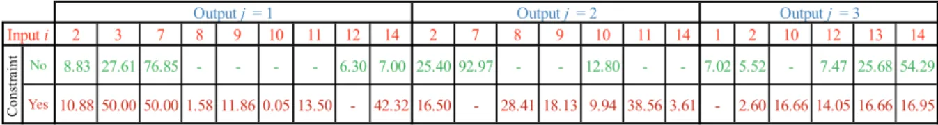
2 3 7 8 9 10 11 12 14 2 7 8 9 10 11 14 1 2 10 12 13 14

No 8.83 27.61 76.85 - - - - 6.30 7.00 25.40 92.97 - - 12.80 - - 7.02 5.52 - 7.47 25.68 54.29 Yes 10.88 50.00 50.00 1.58 11.86 0.05 13.50 - 42.32 16.50 - 28.41 18.13 9.94 38.56 3.61 - 2.60 16.66 14.05 16.66 16.95

Output j = 1 Output j = 2 Output j = 3

C

on

str

aint

4.2 Blending Flexibility in a Dynamic Context

We now turn to a dynamic blending example with alternative routings, inspired from real data (the temporal division used here is the day), in which we determine input feedings to the secondary stock and the optimal blends of inputs to meet 4 output orders performed successively at the same blending unit (the Ben Guerir blending plant has a single blending unit) during a 28-day period( T 28). The secondary stocks of inputs are supplied from primary stocks (see Figure 2) by two conveyors with a flow rate of 4000 T/day, knowing that the same input cannot be conveyed by more than one conveyor, to avoid technical problems when feeding the concerned input stock. We set to 8 the limit KMax of different inputs available

in the secondary stock during the relevant time horizon (relation 12) and the global stock quantity SMax to 150,000 tons. In this problem, constraints on cumulative availability Bc_it

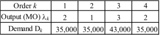
(relation 7) and on minimal stocks are discarded (relation 9). With a daily mixing unit production rate of about 6,200 T, production time for 43,000T of SO to be processed is about 7 days in the dry blending plant. Table 8 describes the production program.

Table 8. Problem data: Order specification

The chosen objective-function only aims to minimize the deviance in outputs 1 and 2 composition to be used subsequently for phosphoric acid production by OCP, using arbitrarily

σ_c   . In this example, one ignores the constraint on minimal stocks by setting θ 0,1, c _i  i

and an arbitrary high cost κ=200,000 is used to avoid dumping storage. The resolution of this

Order k 1 2 3 4

Output (MO) k 2 1 3 2

dynamic blending problem leads to the optimal MO compositions set forth in Table 9 and the optimal secondary stock feeding program from the primary stock shown in Table 10. In this optimal solution, the total internal deviance of internal orders is 921 tons. One notes that the production of OFs 1 and 4, corresponding to the production of 35,000 tons of MO 2 and using routing 2 (washing routing), does not use up the same global quantity of SOs.

Table 9. Optimal Blends

i = 1 i = 2 i = 3 i = 4 i = 5 i = 6 i = 7 i = 8 i = 9 i = 10 i = 11 i = 12 i = 13 i = 14 k= 1j= 1=2 0 2783 0 0 5024 6088 12086 10009 0 0 0 5851 0 0 41840 k= 2j= 2=1 0 2840 12158 0 2150 0 14000 0 2026 0 0 0 0 9330 42504 k= 3j= 3=3 0 0 0 0 1445 0 1286 0 2211 11087 0 1105 8000 17866 43000 k= 4j= 4=2 0 14942 10667 0 0 0 714 0 3574 913 0 0 0 10319 41129  0 20565 22824 0 8620 6088 28086 10009 7811 12000 0 6956 8000 37514 168473 k=1j=1=2 0% 7% 0% 0% 12% 15% 29% 24% 0% 0% 0% 14% 0% 0% 100% k=2j=2=1 0% 7% 29% 0% 5% 0% 33% 0% 5% 0% 0% 0% 0% 22% 100% k=3j=3=3 0% 0% 0% 0% 3% 0% 3% 0% 5% 26% 0% 3% 19% 42% 100% k=4j=4=2 0% 36% 26% 0% 0% 0% 2% 0% 9% 2% 0% 0% 0% 25% 100% xik Input (SO) i i xij / (%) ik i ik x x

Table 10. Optimal feeding program of secondary stock (ρy_it)

Table 9 highlights the differentiation of blend composition of orders 2 and 4 for the same output j1, which illustrates the impact of dynamic blending. Since the transportation capacity of the conveyors is higher than the blending unit’s production capacity, some 6 days without feeding and 9 days requiring use of a single conveyor are reported in (Table 10). These results clearly illustrate that the model avoids transferring from the primary stock any inputs that will not be consumed by the blending, but this does not preclude the building of a sufficient variety in the secondary stock.

4.3 Dynamic Blending Flexibility where alternative routings are combined with Security Stocks

In this section, we illustrate dynamic blending flexibility where alternative routings are

i Si 0 t =1 t =2 t =3 t =4 t =5 t =6 t =7 t =8 t =9 t =10 t =11 t =12 t =13 t =14 t =15 t =16 t =17 1 0 0 0 0 0 0 0 0 0 0 0 0 0 0 0 0 0 0 2 4000 0 0 0 0 0 0 0 0 0 0 4000 0 0 0 0 0 0 3 0 0 0 0 0 0 0 0 4000 0 4000 4000 0 0 4000 0 0 0 4 0 0 0 0 0 0 0 0 0 0 0 0 0 0 0 0 0 0 5 4620 0 0 0 0 0 0 4000 0 0 0 0 0 0 0 0 0 0 6 5032 0 0 0 0 4000 0 0 0 0 0 0 0 0 0 0 0 0 7 4086 0 0 4000 0 4000 0 0 4000 0 4000 0 4000 0 4000 0 0 0 8 15823 0 0 0 0 0 0 0 0 0 0 0 0 0 0 0 0 0 9 7811 0 0 0 0 0 0 0 0 0 0 0 0 0 0 0 0 0 10 0 0 0 0 0 0 0 0 0 0 0 0 0 0 0 4000 4000 0 11 0 0 0 0 0 0 0 0 0 0 0 0 0 0 0 0 0 0 12 6956 0 0 0 0 0 0 0 0 0 0 0 0 0 0 0 0 0 13 0 0 0 0 0 0 0 0 0 0 0 0 4000 0 0 0 4000 0 14 7576 0 0 0 0 0 0 0 0 0 0 0 0 4000 0 4000 0 4000 i Si 0 t =18 t =19 t =20 t =21 t =22 t =23 t =24 t =25 t =26 t =27 t =28 1 0 0 0 0 0 0 0 0 0 0 0 0 2 4000 0 0 0 0 0 4000 4000 4000 4000 4000 0 3 0 0 0 0 0 0 4000 4000 0 0 0 0 4 0 0 0 0 0 0 0 0 0 0 0 0 5 4620 0 0 0 0 0 0 0 0 0 0 0 6 5032 0 0 0 0 0 0 0 0 0 0 0 7 4086 0 0 0 0 0 0 0 0 0 0 0 8 15823 0 0 0 0 0 0 0 0 0 0 0 9 7811 0 0 0 0 0 0 0 0 0 0 0 10 0 0 4000 0 0 0 0 0 0 0 0 0 11 0 0 0 0 0 0 0 0 0 0 0 0 12 6956 0 0 0 0 0 0 0 0 0 0 0 13 0 0 0 0 0 0 0 0 0 0 0 0 14 7576 4000 4000 0 4000 4000 0 0 0 4000 0 4000 36000 37514 6062 0 6956 0 8000 8000 0 12000 12000 0 0 0 0 0 10009 5814 0 7811 0 4000 6088 2944 24000 28086 0 0 0 0 4000 8620 0 24000 20565 7435 24000 22824 1176 0 0 0 Feeding .yit Feeding .yit t yit _WithdrawalsCumulative Si 29

combined with security stocks. 4.3.1 Designing Security stocks

The risk is that of not being able to cope with unexpected demand for merchantable ore where volume corresponds to a week of dry blending production following advanced arrival by one week of a scheduled ship or an unexpected order being placed on the spot market for a small 43,000 tons ore bulk carrier, setting aside such a stock for each merchantable ore is not efficient to say the least. With the flexibility offered by dynamic blending, we can hope to meet such unexpected demand provided we have the minimum source ore stocks described in Table 6, corresponding to flexi-security stocks available to meet any unforeseen orders. This, of course, implies pooling these stocks. We noted that for routings h1, the total amount of source ore and, therefore, the yield (D /_j



_jx_ij ), used for blending, depends on the blend retained in the optimization. Taking into account that the variation of this yield is not large, that dry blending production flow can be momentarily increased versus its nominal value (from 40,000 to 48,000 tons / week) and, finally, that integration into the production schedule of an urgent order may be addressed by shifting the following orders according to production time, one can reasonably simplify the problem through an average yield rate η_j2



_ix_ij* .η /D_{i2 j}, for routing

2

h ,by using the optimal solution x of blending problem without any constraint; here, we _ij*

use η_j20.77 Since we consider a short-term horizon (lower than 6 weeks), the constraint on cumulative availability (relation 7) is eliminated.

Let us turn to the analysis of Table 6 showing minimum merchantable ore production volume. That table shows that SO 2 is necessary to produce MO 1 (minimum 3%) and 4 (minimum 8%). Therefore, in order to respond to an urgent contingency order for any MO, we must have a 3,340-tons SO 2 security stock (Max 45,000 3%;43,000 8%



 



3,440). In the absence of such a security stock for SO 2 it is impossible to produce both MO 1 and MO 4. The

ceiling level for minimum required quantities of each input (SO), shown in Table 6, can be analysed as a security stock in an uncertain environment.

This risk mitigation strategy designed to address an urgent and unexpected order, involves: i) security stocks for indispensable SOs to manufacture certain MOs and ii) the flexibility provided by dynamic blending to adjust output composition according to demand characteristics, combined with immediately available input stocks and availability of feeding stocks from SO ready to be removed from the mine over the next few weeks (formulation in §3.1). For all these reasons, security stocks presented here address both types of risk coverage in uncertain environment. Nevertheless, note that there remains a risk that one will not be able to fulfil an order where other, optional, SO are not available in sufficient quantity to produce one of the possible alternative blends.

4.3.2 Illustration of the flexibility delivered where dynamic blending with alternative routings is combined with security stocks

We rely on the same problem reference data as that introduced in part §4.2. In order to highlight dynamic blending flexibility of where alternative routings are combined with security stocks, two cases have been considered; the first without constraint on safety stocks and the other, where there are constraints on safety stocks.

We proceeded in the same way as in Case I to define the optimal solutions for Case II. The deviance observed for internal MO orders for both cases before introduction of unexpected orders is reported in Table 11.

Table 11. Total Deviance of Internal MOs

Table 11 clearly shows that total internal deviance for Case II is better than that for Case I.

We have supposed that, during Period 14, we received an urgent order after completion of the first two scheduled orders. We examined the feasibility of meeting orders at the beginning of Period 15 (Scenarios A and B). Since production time for urgent orders is quite constant (about 7 days), two scenarios for these unexpected situations, the most probable ones, have been reviewed in this study:

• Scenario A: replace an external order by an internal one (here we replaced order k=3 for external MO j=3 with another concerning internal MO j=1);

• Scenario B: add an exceptional order for an internal MO (here orders k=3 and k=4 are postponed by about a week to satisfy order k=5 for internal MO j=1).

Whatever the scenario, we ignore all new information beyond the horizon adopted, even if shifting orders implies exceeding it. In fact, we do not extend site availability accumulation B_it

. Our initial stock for both scenarios was therefore equal to that at the end of the period 14

, 14

(S_{i t} ). For scenario B, the accumulation of the prepared SOs in primary stocks for periods beyond period t28was equal to the accumulation of prepared SOs for period 28, that is

, 28 , 28 B_{i t} B_{i t} c = 1 c = 2 c = 3 c = 4 c =5 Deviance of internal MO Deviance of internal MO Deviance of internal MO Deviance of internal MO Deviance of internal MO k = 1 314 0 35 163.39 0 512.39 k = 2 197.95 0 35 175 0 407.95 k = 4 0 0 0 0 0 0 k = 1 250.12 0 35 175 0 460.12 k = 2 0 0 35 166.83 0 201.83 k = 4 0 0 0 0 0 0 Components Internal MO T otal Deviance Internal orders Constraint on Security Stock Case I No II Yes