Dynamic blending as a source of flexibility and efficiency in controlling phosphate supply chain

lamsade

LAMSADE

Laboratoire d’Analyse et Modélisation de Systèmes pour

l’Aide à la Décision

UMR 7243

Avril 2017

A. Azzamouri, V.Giard

CAHIER DU

381

Dynamic blending as a source of flexibility and efficiency in controlling phosphate supply chain

Dynamic blending as a source of flexibility and efficiency in

controlling phosphate supply chain

Vincent Giard1&2_{, Ahlam Azzamouri}3,

1. Emeritus Professor at Paris-Dauphine, PSL Research University – LAMSADE 2. Affiliated Professor at l'EMINES School of Industrial Management, OCP

Industrial Optimization chair

3. PhD student at EMINES School of Industrial Management

Abstract. The phosphate extraction process of at the Ben Guerir deposit feeds 14 ore stocks of

different chemical characteristics. The production decisions impact the replenishment of these stocks, which can be strongly delayed in time. The ore demand to be met for the export or production of phosphoric acids does not concern these primary ores but blended ore grades matching certain chemical characteristics. The cost of this transformation is not very sensitive to required grade and many possible blending “recipes” lead to the same end product (blended ore grade). The structure of this grade demand fluctuates over time and orders are known only a few weeks in advance. The stock replenishments of extracted ores are strongly irregular. This paper shows that degrees of freedom in blend structure, unfortunately often ignored, are available: 1) to meet demand while limiting recourse to emergency procedures to offset ore shortages; 2) to limit temporary storage of quantities of certain produced ores due to insufficient storage space in the blending zone. Mathematical programming can be used to define tailored blends based on available ores to meet grade demands within a few weeks, and so avoiding or limiting costs induced by use of a standard blend of extracted ores. This is illustrated by a number of examples1_{. The parameterization used in the formulation of the} problem enables instantaneous adjustment to any change in the characteristics of the extracted ores and required grades.

1 _{This part and the references study were written in collaboration with the student of the PhD program of EMINES: Meryem}

Bamoumen, Mouna Bamoumen, Najat Bara, Latifa Benhamou, Lamiaa Dahite, Hajar Hilali and Asma Rakiz

Keywords. Blending; Supply chain; Make-To-Order; sequential inputs supply.

I. Introduction

The Ben Guerir open pit phosphate mine produces N 14= different ores ( 1..N)i =

that are extracted from as many homogeneous layers. Each layer i is characterized by specific values α_ci of geological components c ( 1..6)c = (see table 1). The extracted ores are inputs used to produce blended ores (outputs j,

1..J)

j = whose component composition β_cj must comply with a quality chart (see a sample of such a chart in table 2). Those blended ores, whose variety is increasing, are used downstream in the phosphoric supply chain (SC) of OCP, which owns the largest phosphate ore deposits in the world.

Table. 1. Input composition (extracted ores) in % of their weights (α_ci) c =1 BPL MGOc =2 SIOc =32 c =4 H2O c =5 CO2 c =6 Cd/B (ppm) i =1 C3 sup 50.01% 0.99% 26.61% 0.00% 3.70% 8.00 i =2 SA2 57.87% 0.65% 8.00% 0.00% 7.74% 15.00 i =3 C3G 58.95% 0.94% 17.19% 0.00% 5.36% 9.00 i =4 C1 59.50% 1.15% 9.50% 0.00% 4.50% 15.00 i =5 C0 59.50% 1.20% 8.61% 0.00% 5.20% 13.00 i =6 C4 59.50% 1.49% 11.74% 0.00% 4.83% 10.00 i =7 C5 59.60% 1.70% 9.79% 0.00% 7.72% 16.00 i =8 C2 sup 60.00% 0.91% 11.50% 0.00% 5.08% 12.00 i =9 SB 61.50% 0.80% 8.00% 0.00% 5.24% 10.00 i =10 SX 63.00% 0.80% 11.00% 0.00% 5.50% 10.00 i =11 C3 inf 64.00% 1.12% 10.00% 0.00% 4.95% 8.00 i =12 C1 Exp 65.50% 1.13% 7.50% 0.00% 4.25% 12.00 i =13 C2 Exp 65.50% 0.65% 8.00% 0.00% 4.61% 13.00 i =14 C6 65.72% 1.23% 6.00% 0.00% 4.95% 9.00 Component c Inpu ti

Table. 2. Sample of specifications of outputs composition (β_cj) c =1 BPL MGOc =2 c =3 SIO2 c =4 H2O c =5 CO2 c =6 Cd/B (ppm) j=1 TBT 54.00- 56.00 <=2.00 <=15.00 - - -j=2 YCC > 64.00 <= 1.00 <= 8.00 < 12.00 5.00 - 6.00 12.00 - 18.00 j=3 BG 57.90 < 1.40 <=13.50 - - < 11.50 Component c O ut pu tj

In the OCP integrated supply chain, the blending problem is more complex than that faced by companies sourcing inputs from the market for the following two reasons:

a. Phosphate market development trends are characterized by an increased diversity of the technical specifications of the required grades, in a highly competitive market. This leads to production to order, wherever the associated production lead time is commercially acceptable (which is the case for OCP’s SC).

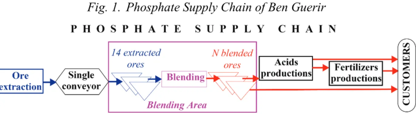
b. The ores extracted from the different layers are transported to a single stripping station before conveyor transport to the blending area to be stored in one of the 14 stocks dedicated to the different qualities of extracted ores (Fig. 1). Since this process of separation and transport does not allow any mixing, this leads to sequential feeding of these stocks. The allocation of storage space to the 14 extracted ores varies over time but can be considered as known during a period of a few weeks. In case of insufficient storage for a given quality, the extracted ore concerned is temporarily stored in a remote dumping

stock, in the vicinity of the stone screening plant, before being retrieved when the space becomes available. These steps are costly and add no value.

Fig. 1. Phosphate Supply Chain of Ben Guerir

The definition of the optimal composition of blended products, which minimizes the product costs, was one of the very first problems to be addressed by linear programming in the 1950’s and this remains the single focus of the industrial management and operation research text books .

The stability of product composition obtained by blending is rational in a steady state where the needs to be satisfied and conditions of acquisition of the inputs are stable and unrestricted (although this “steady state” needs to be re-assessed once or twice a year). OCP, however, is not in this situation and the fixed composition of output blends causes loss of efficiency and effectiveness. We will show how to take advantage of the multiple opportunities for flexible product blending to enhance system performance.

In section II, we present our analysis of the literature. Our proposed blending models are described in Section III. Section IV illustrates the importance of blending flexibility and discusses some of the factors explaining why, for optimization reasons, blended ore composition cannot be stable. We end with a short conclusion (Section V).

II. Literature review of blending problems

The articles we analyzed deal with blending issues in various sectors, namely mining [5] [9] [15], agri-foods [13] [14] [16], milling [3][8], chemistry[1][7][6][11], tanker [2] [4] [12], cementitious [10]. All the articles reviewed were evaluated mainly with reference to the following three criteria: • The type of input feeding: there are two types of feeding: 1. Blending units

fed through single conveyors, which defines a sequential (successive) arrival of inputs. This is illustrated by the case of bulk grain Blending [3], semi-continuous blending of materials [6] and blending of raw materials to produce raw cement meal [10]. A parallel feeding of the inputs is illustrated by the case of fertilizer blending [1], crude oil [2] [12], sausages [13], coking coal [15].

rationale of: 1). Pull flow which means that blending is performed in order to meet a specific need expressed by an internal or external client

(Make-to-order); this case is illustrated by articles [2] [3] [5] [8] [12] [13] [14] [15]. 2).

Push flow which means to produce for stock or make to stock, which is the

case in articles [1] [10].

• The optimization criterion: differs from article to article, depending on the type of blending. Some articles adopt the optimization criterion for either production or running costs as illustrated by articles [1] [4] [9 [16]. Others seek to minimize the cost of transport [3], or maximize profit as illustrated by articles [2] [12]. Other papers dealing with blending focus on quality [11] [7], while others combine cost and quality criteria [9] [8] [14] or the three criteria cost, quality and profit [13]. Moreover, the minimization of penalties incurred due to any deviation from target values is also a resolution criterion addressed in certain articles [5] [6] [10].

Based on our analysis of the articles we were able to confirm that our paper addresses a blending issue that combines several features: inputs with characteristics that differ over time, irregular availability and sequential feeding of input stocks with limited capacity. These constraints must be taken into account in order to make to order with a sequential feeding of output stocks. Moreover, our paper differs from the literature reviewed on grounds of the resolution criteria we adopted which, in addition to cost, addresses the issue of scarcity, which roughly consists in the conservation of the BPL-rich layers.

III. Formulation of the Blending Problem

In its classic formulation, blending aims at defining the optimal mixture of selected inputs in a set of N possible inputs( 1..N),i = taken in quantities x_i to

obtain quantity D=

∑

_ix_i of a unique output that complies with the

composition’s specifications. The weight of component c in the output obtained by blending, β_c =

∑

_cα_{ci i}⋅x may have to belong to a range of values. In this static modeling, input i has an acquisition cost γ_i and the problem here is to find the blend that minimizes the cost of acquisition

∑ ∑

_iγ_{i j}x_ij . Since the problem variables are continuous, there is an infinite number of possible solutions or none, if the problem is unfeasible.

The particular context of the supply chain in which the blending problem occurs (sequential feeding of inputs, make-to-order) leads to a dynamic reformulation of this problem based on splitting time into periods( 1..T)t = . The scheduling of a set of K production orders fulfilled in parallel blending processors is assumed to be already established and compliant with processor availability; this leads to ignoring the processors in our formulation. The order variable x_ik

corresponds to the weight of input i included in the weight D_kof order k, for output λ_k, which leads to constraint (1).

D

ik k ix =

∑

(1)

Since the output portfolio changes rapidly, the constraints on the structure of the components are described generically in 3 tables of parameters for each component c of output j: βEq_cj , βMin_cj et βMax_cj . These parameters take a positive value if component c constrains the composition of output j, the first in the case of equality and the other two in the case of inequality. All these composition constraints are given by relation (2), which is easily used in a problem formulation using an AML (Algebraic Modeling Language) which allows to use predicates in the generation of variables and constraints.

Eq Eq Min Min Max Max α β D , |β 0 α β D , |β 0 α β D , |β 0 k k k k k k ci ik _c k _c i ci ik c k c i ci ik c k c i x k x k x k λ λ λ λ λ λ ⋅ = ⋅ ∀ ≠ ⋅ > ⋅ ∀ ≠ ⋅ < ⋅ ∀ ≠

∑

∑

∑

(2) The fulfillment of order k leads to the withdrawal of inputs during periods t such as δ_kt =1 (otherwise, this Boolean equals 0); the duration of withdrawal is notedν_k (

∑

_tδ_kt =ν )_k . Changes in stock S ≥_it 0 of input i at the end of period t depends on the initial stockS_i0, the supplies A_it′ available at the beginning of the period t t′ ≤ and the withdrawals of this input during periodt t′ ≤ . It will be assumed here that withdrawal is constant over the ν_k withdrawal periods (otherwise it is necessary to introduce dated coefficients, which does not change the size of the problem). Relations (3) reflect this flow conservation constraint.

, , 1 _{| 1} / ν , , 0, , kt i t i t it _k ik k it S S A x i t S i t δ − ₌ = + − ∀ ≥ ∀

∑

₍₃₎

We will examine two formulations of the dynamic blending problem; the second formulation complements the first one in an attempt to avoid, through flexible blending, any unnecessary costs due to temporary storage (cf. § III.2).

III.1 General formulation ignoring blending area storage constraints

In the productive system under review, direct blending costs are not very sensitive to the solution, which lead us to look for the best solution while sparing future resources. This approach amounts to preserving the scarcest ores at the end of period T. In our numerical examples, we use arbitrarily the weighting system

1

i i

γ α= , where the index c=1 corresponds to the BPL content, which leads to objective-function (4).

T

( _{i i i} )

Max

∑

γ ⋅S (4)

In order to assess the different blending options available, some variants of this general model are used. They include as many orders as available processors and they leave time considerations aside, which implies input feeding as stocks S_i0 is deemed sufficient. The result is a static problem with five variants. Variants A to

D concern the blending problem for a single order j , without any input ₀

availability issue; variant E relates to multiple orders where there are availability constraints.

- Variant A: Is a basic static model with a single order, using objective-function (4).

- Variant B: replaces objective-function (4) by the minimization

0 0

(Min x( _kj / D ))_j or by the maximization (Max x( _kj0 / D ))_j0 of input % i k= ( 1..N)k = in the weight of j₀, which leads, in our example, to 28 optimizations per output studied.

- Variant C: forcing the blending process to use a predetermined number H of inputs; in this context; the binary variable z =_ij0 1 if input i is used, which is obtained with relation (6); the additional constraint (7) forces the number of inputs used in the blending to be H. In variants B and C, objective- function (4) is replaced by objective-function (5) 0 ( _{i i ij} ) Min

∑

γ ⋅x (5) 0 0 0 D_j ⋅z_ij <x_ij ,∀i (6) 0 H ij iz =

∑

(7)

- Variant D: setting to 0 the stock for the most requested input in the current solution, and identification of an alternative new blend; this process, which complies with the minima of variant B, starts from the solution corresponding to the lowest value of H found in variant C and goes on until it is no longer possible to find a solution.

- Variant E: also static, covers several orders fulfilled simultaneously and assesses the impact of insufficient availability of inputs to achieve optimal solutions for variant A.

III.2 General formulation taking into account the storage constraints in the blending area

Dumping storage of input i takes place as soon as the stock exceeds threshold Max

Max 0, , it it it i y i t y S S > ∀ > − (8)

The benefit of avoiding such dumping storage prevails on that of preserving stocks of the ores deemed most valuable. The system used to calculate the cost of dumping storage is irrelevant so long as dumping can be avoided (as the corresponding partial cost in the objective function is null). We shall use storage cost η, proportional to both the duration of the dumping storage and to stored quantities. This leads to replace relation (4) by relation (9).

T

(η _{t i it i i i} )

Min ⋅

∑ ∑

_′ y _′+

∑

γ ⋅S (9)

IV. Illustration of blending flexibility

We illustrate below blending flexibility first in a static context (production during a single period), then in a dynamic context.

IV.1 Blending flexibility in a static context

We illustrate the importance of blending flexibility first in the case of a single output (§a), then in the case of multiple outputs (§b). We use the data from tables I and II.

a) Blending flexibility within the framework of a single output

In variants A to C, we use D 100,_j = ∀j andS_0i =100,∀i, which prevents the risk of stockout and allows considering x_ij as percentages.

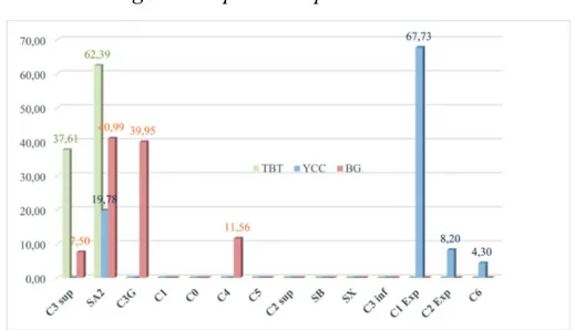
Variant A. the optimal blending solutions (Fig.2) were obtained successively

and independently, using objective function (4), for each one of the products.

Variant B. The minimal and maximal shares of the different inputs in

manufacturing each output, where all inputs are deemed available, are given in table 3. This in fact undermines the scarcity criterion based on BPL content, since one observes that TBT cannot be produced without C3sup and SA2, and that BG requires C3sup, while both inputs have the lowest BPL content. Furthermore, YCC must include C2sup, a substance that has the median BPL content of all inputs.

Table. 3. Minimal and maximal quantities of inputs for each output i =1

C3sup SA2i =2 C3Gi =3 i =4C1 i =5C0 i =6C4 i =7C5 C2supi =8 i =9SB i =10SX C3infi =11 C1Expi =12 C2Expi =13 i =14C6

Quantity Min 23.79 6.71 - - - -Quantity Max 39.28 76.21 21.91 48.00 57.56 33.86 43.70 30.11 29.93 16.98 15.58 14.64 14.24 15.51 Quantity Min _{- - - - - - - - - - - - 3.24} -Quantity Max 3.05 20.68 5.85 16.36 20.73 11.67 22.31 14.92 29.36 14.56 14.92 67.73 87.54 39.57 Quantity Min _{7.50 - - - - - - - - - - - -} -Quantity Max 33.16 50.00 42.24 42.89 70.00 73.32 34.30 55.07 64.82 36.64 33.74 25.74 21.27 33.59 Inputs i O ut pu ts j TBT j=1 YCC j=2 BG j=3

Variant C. This represents successively for each output the range of the

number of inputs that are adequate to produce a given output. The results are shown in Table 4. The minimum number of inputs required to produce an output may be less than that found in the optimal solution for variant A, at the cost of undermining performance. (Case of YCC which can be manufactured with just 2 inputs and of BG which can be made with just 3 inputs.) For TBT, this minimum number corresponds to that of the optimal solution. For each output, the maximum number of inputs indicated in this table cannot be exceeded without violating the composition specifications for the relevant output. In conclusion, the

number of inputs used to produce an output can be much higher than the number of inputs used without constraint (variant A).

Table. 4. Possible blends depending on a compulsory number of inputs to be

used i =1

C3sup SA2i =2 C3Gi =3 i =4C1 i =5C0 i =6C4 i =7C5 C2supi =8 i =9SB i =10SX C3infi =11 C1Expi =12 C2Expi =13 i =14C6 2 inputs 37.61 62.39 - - - -3 inputs -35.15 59.85 5.00 - - - -4 inputs 3-4.7-4 55.26 5.00 5.00 - - - -5 inputs 34.-58 -50.42 -5.00 -5.00 -5.00 - - - -6 inputs 33.57 4-6.43 5.00 5.00 5.00 5.00 - - - -7 inputs 33.09 41.91 5.00 5.00 5.00 5.00 5.00 - - - -8 inputs 32.15 37.-85 5.00 5.00 5.00 5.00 5.00 5.00 - - - -2 inputs - 19.65 - - - 80.34 -3 inputs - 19.65 - - - 62.59 17.74 -4 inputs - 19.78 - - - 67.72 8.19 4.29 5 inputs - 19.45 - - - 1.00 - 67.38 7.84 4.32 6 inputs - 19.25 - - - 1.00 1.00 66.51 7.99 4.23 7 inputs - 18.43 - - - - 1.00 - - 1.00 1.00 66.38 9.65 2.52 8 inputs - 17.63 1.00 - - - 1.00 - - 1.00 1.00 63.37 10.46 4.52 9 inputs - 17.13 1.00 - - - 1.00 - 1.00 1.00 1.00 61.81 10.49 5.56 10 inputs - 16.40 1.00 - 1.00 - 1.00 - 1.00 1.00 1.00 58.67 11.72 7.24 3 inputs 15.43 - 24.62 - 59.95 - - - -4 inputs 7.50 40.99 39.95 - - 11.56 - - - -5 inputs 8.04 38.09 39.38 - 5.00 9.49 - - - -6 inputs 9.17 38.20 37.63 - 5.00 5.00 - - 5.00 - - - - -7 inputs 10.13 33.21 35.-79 5.00 5.00 5.86 - - 5.00 - - - - -8 inputs 11.04 30.79 31.-8-8 5.00 5.00 6.29 - 5.00 5.00 - - - - -9 inputs 13.26 30.54 26.20 5.00 5.00 5.00 - 5.00 5.00 5.00 - - - -10 inputs 16.11 28.51 20.34 5.00 5.00 5.05 5.00 - 5.00 5.00 5.00 - - -11 inputs 17.01 26.09 16.42 5.00 5.00 5.47 5.00 5.00 5.00 5.00 5.00 - - -12 inputs 21.03 24.00 7.93 5.00 5.00 7.05 5.00 5.00 5.00 5.00 5.00 5.00 - -Inputs i O ut pu ts j j= 1 TB T j= 2 Y C C j= 3 B G

Variant D. This represents successively the impact of zero stocks for some

inputs for each output (the positive minima of variant C being retained). This places us before a highly combinatorial problem (C problems). Therefore, we ₁₄k have opted for a scenario where i) we start from the optimal solution found with stocks set to minimum in table III, the others being at 100; ii) we set to zero initial stock for the most requested input in the previous optimal solution; iii) we look for the new optimal solution, and if one is found, we return to ii), if not we stop.

Table. 5. Possible blends depending on input availability i =1 C3sup i =2 SA2 i =3 C3G i =4 C1 i =5 C0 i =6 C4 i =7 C5 i =8 C2sup i =9 SB i =10 SX i =11 C3inf i =12 C1Exp i =13 C2Exp i =14 C6 Initial stock 100 100 100 100 100 100 100 100 100 100 100 100 100 100 Blending 37.61 62.39 - - - -Initial stock 23.79 100 100 100 100 100 100 100 100 100 100 100 100 100 Blending 23.79 76.21 - - - -Initial stock 100 6.72 100 100 100 100 100 100 100 100 100 100 100 100 Blending 35.73 6.72 _- 0.02 57.53 _{- - - - - - - -} -Initial stock 100 6.72 100 100 - 100 100 100 100 100 100 100 100 100 Blending Initial stock 100 100 100 100 100 100 100 100 100 100 100 100 100 100 Blending - 19.78 - - - 67.73 8.19 4.29 Initial stock 100 100 100 100 100 100 100 100 100 100 100 100 3.24 100 Blending 0 14.71 0 0 0 0 0 0 0.99 14.02 0 61.35 3.24 5.69 Initial stock 100 100 100 100 100 100 100 100 100 100 100 - 3.24 100 Blending Initial stock 100 100 100 100 100 100 100 100 100 100 100 100 100 100 Blending 7.50 40.99 39.95 - - 11.56 - - - -Initial stock 7.50 _- 100 100 100 100 100 100 100 100 100 100 100 100 Blending Initial stock 7.50 100 _- 100 100 100 100 100 100 100 100 100 100 100 Blending Inputs O ut pu ts j= 1 TB T No possible blend j= 2 Y C C No possible blend j= 3 B G No possible blend No possible blend

Following the approach explained in variant D, we reach the following

conclusions:

C3sup and SA2 to their minima, we don’t obtain a feasible solution. Therefore, we address these stocks successively. As a matter of fact, when first setting the stock of input C3sup at its minimum, we still come out with a possible blend using the quantities of both two inputs C3sup and SA2. The second step, when setting stock of input SA2 to a minimum, again we obtain a feasible solution that involves consumption of input C0. Lastly, while keeping SA2 stock to a minimum and setting stock of input C0 to zero, we don’t find any solution enabling production of output TBT.

As for product YCC, this can be obtained when setting initial stock of input C2Exp to its minimum. In this case, the solution found uses an important quantity of input C1Exp. As a second step, while maintaining stock of C2Exp to its minimum and putting stock of C1Exp to zero, we don’t find any possible blend to produce output YCC.

For product BG, we note that when setting stock of input C3sup to its minimum, a solution that involves consumption of inputs SA2 and C3G is still possible. However, while maintaining stock of C3sup to a minimum and successively setting SA2 and C3G stocks to zero, we don’t come up with a feasible solutions in either case.

To conclude, output production is still possible where some inputs are not

available (within the minima shown in Table III).

b) Blending flexibility within the framework of a several outputs

Variant E. This deals with three orders fulfilled simultaneously, for equal

quantities of 100, with each input availability remaining set at 100. The aggregation of input consumptions for the solutions found in variant A leads to stock-out of SA2 (table 6). Considering that constraint (6) leads to new blends for which the selected optimization criteria involve input SA2 shortage for output BG.If we completely change input allocations (table 7), we obtain blends that are very different from those of Table 6. To conclude, the blends of outputs produced

Table. 6. Mono-period/multi-product model with distinctD_k and S_i0

TBT YCC BG Sum TBT YCC BG Sum C3 sup 100 37.61 3.04 33.16 73.81 37.61 3.03 32.26 72.90 SA2 100 62.39 14.11 33.25 109.75 62.39 14.11 23.51 100 C3G 100 - - - -C1 100 - - - -C0 100 - - - 14.57 14.57 C4 100 - - - -C5 100 - - - -C2 sup 100 - - - -SB 100 - - - -SX 100 - - - -C3 inf 100 - - - -C1 Exp 100 - 27.01 - 27.01 - 27.01 - 27.01 C2 Exp 100 - 34.33 - 34.33 - 34.33 - 34.33 C6 100 - 21.51 33.59 55.10 - 21.52 29.66 51.18 100 100 100 300.00 100 100 100 300.00 Free optima of variante A Orders (outputs) I n p u t s i Sum Optima of variante F Orders (outputs) 0 i S

Table. 7. Mono-period/multi-product model with distinct D_k and S_i0

TBT YCC BG Sum TBT YCC BG Sum TBT YCC BG C3 sup 50 36.52 3.84 16.58 56.93 36.25 1.25 12.50 50.00 36.2% 0.8% 25.0% SA2 30 30.00 11.60 16.62 58.23 21.96 8.04 - 30.00 22.0% 5.4% -C3G 20 - - - 4.27 - 4.27 - 2.8% -C1 50 - 6.86 - 6.86 - 12.62 16.32 28.94 - 8.4% 32.6% C0 50 33.48 - - 33.48 41.79 - 8.21 50.00 41.8% - 16.4% C4 20 - - - 6.76 6.76 - - 13.5% C5 20 - 7.58 - 7.58 - 8.47 - 8.47 - 5.6% -C2 sup 0 - - - -SB 0 - - - -SX 0 - - - -C3 inf 0 - - - -C1 Exp 30 - 30.00 - 30.00 - 22.68 - 22.68 - 15.1% -C2 Exp 50 - 50.00 - 50.00 - 50.00 - 50.00 - 33.3% -C6 50 - 40.12 16.79 56.92 - 42.67 6.21 48.88 - 28.4% 12.4% 100 150 50 300.00 100 150 50 300.00 100.0% 100.0% 100.0% I n p u t s i Sum Free optima of variante A Orders (outputs) Optima xij of variante F Orders (outputs) Optima (% blend) of variante F Orders (outputs) 0 i S

IV.2 Dynamic Blending Flexibility

Let us arbitrarily consider the blending of 6 orders fulfilled by 2 blending units running simultaneously. The time split selected is 16 half-days. The processor speed is 10 units / half day. We consider that during the last scheduled period of an order there is no input supply as this final period is dedicated to the completion of the final mixture. Table 8 presents the data for the production sequence problem: initial stocks of inputs, (sequential) feeding of input stocks.

Table. 8. Problem Data

i =1

C3sup SA2i =2 C3Gi =3 i =4C1 i =5C0 i =6C4 i =7C5 C2supi =8 i =9SB i =10SX C3infi =11 C1Expi =12 C2Expi =13 i =14C6 40 50 50 50 50 50 30 50 50 50 50 50 50 50

Initial inventory of inputs i

0 S_i 0 S_i Period t 1 2 3 4 5 6 7 8 9 10 11 12 13 14 15 16 i =1 C3sup - - - 10 10 - - - -i =2 SA2 - - - 10 10 - - - -i =3 C3G - 10 10 - - - -i =12 C1Exp - - - 10 10 10 - - 10 10 - - - -i =8 C2sup 10 - - - -i =13 C2Exp - - - 10 10 i =14 C6 - - - 10 10 -

-Sequential feeding Aitof input stocks i

Begin End j=1 1 TBT 40 1 5 j=2 1 YCC 30 6 9 j=3 1 TBT 50 10 15 j=4 2 TBT 60 1 7 j=5 2 BG 40 8 12 j=6 2 YCC 30 13 16 Orders specifications Quantity Output

Orders j Processor Production period

a) Example ignoring blending area storage constraints.

The use of objective-function (4) leads to the solution described in Table IX. We note that the blends of the three TBT orders are different, which has to do with the structure of the problem data since blending now depends on input

availability and on the fact that outputs are competing for consumption of the same inputs.

Table. 9. Solution without attempt to avoid dumping storage 1

(TBT) (YCC)2 (TBT)3 (TBT)4 (BG)5 (YCC)6 (TBT)1 (YCC)2 (TBT)3 (TBT)4 (BG)5 (YCC)6

C3 sup 13.51 - 16.96 21.41 4.73 0.00 56.61 33.77% - 33.91% 35.69% 11.83% -SA2 9.48 5.90 13.28 16.85 17.46 4.39 67.34 23.70% 19.66% 26.56% 28.08% 43.64% 14.62% C3G - - - - 14.98 - 14.98 - - - - 37.46% -C1 - - - -C0 - - 18.50 - - - 18.50 - - 37.00% - - -C4 - - - -C5 16.00 - - 12.00 - 1.50 29.50 40.00% - - 20.00% - 5.00% C2 sup - - - -SB 1.01 - - 9.74 - - 10.75 2.54% - - 16.23% - -SX - - - -C3 inf - - - -C1 Exp - 18.78 - - - 18.59 37.37 - 62.59% - - - 61.98% C2 Exp - 5.32 1.26 - - 5.52 12.11 - 17.75% 2.52% - - 18.40% C6 - - - - 2.83 - 2.83 - - - - 7.08% -40.00 30.00 50.00 60.00 40.00 30.00 250.00 100.00% 100.00% 100.00% 100.00% 100.00% 100.00% Sum

Inputs consumptions Blend structure of outputs

Orders (outputs) Sum Orders (outputs) I n p u t s

b) Example taking into account blending area storage constraints.

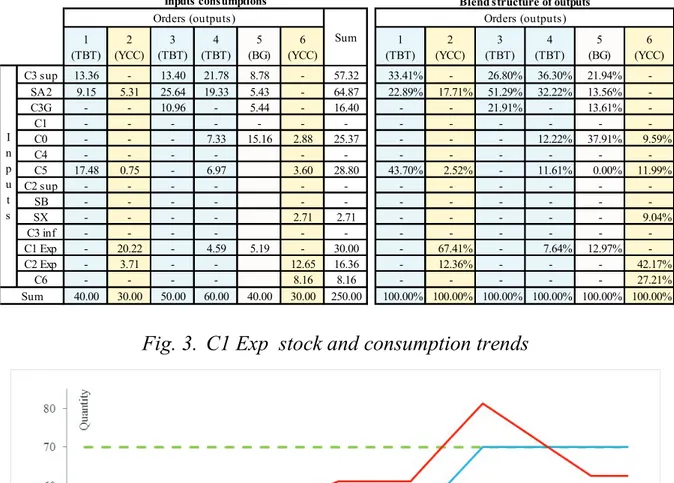
Using objective-function (9) with η 10= and capacity constraint only relevant for the 12th _{input C1 Exp} Max

12

(S =70) leads to the solution described in table 10. Without taking into account the costs incurred by C1 Exp dumping storage (green dotted line of Fig. 3), an overrun at period 12 (red continuous line, solution of §a) is observed. Taking these costs into account in objective function (9) changes total consumption for this input and smoothes consumption in order to meet the availability constraint. All blends are accordingly changed. Taking storage constraints into account to avoid non value-added operations is an additional source of blending change.

Table. 10. Optimal solution to avoid dumping storage 1

(TBT) (YCC)2 (TBT)3 (TBT)4 (BG)5 (YCC)6 (TBT)1 (YCC)2 (TBT)3 (TBT)4 (BG)5 (YCC)6

C3 sup 13.36 - 13.40 21.78 8.78 - 57.32 33.41% - 26.80% 36.30% 21.94% -SA2 9.15 5.31 25.64 19.33 5.43 - 64.87 22.89% 17.71% 51.29% 32.22% 13.56% -C3G - - 10.96 - 5.44 - 16.40 - - 21.91% - 13.61% -C1 - - - -C0 - - - 7.33 15.16 2.88 25.37 - - - 12.22% 37.91% 9.59% C4 - - - -C5 17.48 0.75 - 6.97 3.60 28.80 43.70% 2.52% - 11.61% 0.00% 11.99% C2 sup - - - -SB - - - -SX - - - - 2.71 2.71 - - - 9.04% C3 inf - - - -C1 Exp - 20.22 - 4.59 5.19 - 30.00 - 67.41% - 7.64% 12.97% -C2 Exp - 3.71 - - 12.65 16.36 - 12.36% - - - 42.17% C6 - - - - 8.16 8.16 - - - 27.21% 40.00 30.00 50.00 60.00 40.00 30.00 250.00 100.00% 100.00% 100.00% 100.00% 100.00% 100.00% I n p u t s Sum Sum Orders (outputs) Blend structure of outputs Inputs consumptions

Orders (outputs)

V. Conclusion

The multiple blending options enabled by dynamic blending management, based on orders and input stocks and feeding changes improve effectiveness (more opportunities to meet demand) and efficiency (avoid costly operations without added value), compared with monitoring based on standard blend structures. This flexibility can also be used in extraction control, as the coupling of customer demand (downstream of blending) and phosphate extraction (upstream of blending) should not be deemed rigid. We also note that our proposed modeling can easily be tailored to include both granularity (important in the later stage of chemical transformation) and order scheduling (considered as known in this paper).

VI. References

[1] J. Ashayeri, A. G. M. van Eijs, et P. Nederstigt, “Blending modelling in a process manufacturing: A case study”, European Journal of Operational Research, vol. 72, no 3, p. 460-468, févr. 1994.

[2] J. Bengtsson, D. Bredström, P. Flisberg, et M. Rönnqvist, “Robust planning of blending activities at refineries”, The Journal of the Operational Research Society, vol. 64, no 6, p. 848-863, 2013.

[3] B. Bilgen et I. Ozkarahan, “A mixed-integer linear programming model for bulk grain blending and shipping”, International Journal of Production Economics, vol. 107, no 2, p. 555-571, juin 2007.

[4] M. Cain et M. L. R. Price, “Optimal Mixture Choice”, Journal of the Royal Statistical Society. Series C (Applied Statistics), vol. 35, no 1, p. 1-7, 1986.

[5] E. K. C. Chanda et K. Dagdelen, “Optimal blending of mine production using goal programming and interactive graphics systems”, International Journal of Surface Mining, Reclamation and Environment, vol. 9, no 4, p. 203-208, janv. 1995.

[6] P. L. Goldsmith, “The theoretical performance of a semi-continuous blending system”, Journal of the Royal Statistical Society. Series D (The Statistician), vol. 16, no 3, p. 227– 251, 1966.

[7] S. Jonuzaj et C. S. Adjiman, “Designing optimal mixtures using generalized disjunctive programming: Hull relaxations”, Chemical Engineering Science, vol. 159, p. 106-130, février 2017.

[8] U. S. Karmarkar et K. Rajaram, “Grade Selection and Blending to Optimize Cost and Quality”, Operations Research, vol. 49, no 2, p. 271-280, 2001.

[9] M. Kumral, “Application of chance-constrained programming based on multi-objective simulated annealing to solve a mineral blending problem”, Engineering Optimization, vol. 35, no 6, p. 661–673, 2003.

[10] A. Kural et C. Özsoy, “Identification and control of the raw material blending process in cement industry”, International Journal of Adaptive Control and Signal Processing, vol. 18, no 5, p. 427–442, 2004.

[11] G. Montante, M. Coroneo, et A. Paglianti, “Blending of miscible liquids with different densities and viscosities in static mixers”, Chemical Engineering Science, vol. 141, p. 250-260, févr. 2016.

[12] T. A. Oddsdottir, M. Grunow, et R. Akkerman, “Procurement planning in oil refining industries considering blending operations”, Computers & Chemical Engineering, vol. 58, p. 1–13, 2013.

[13] R. E. Steuer, “Sausage Blending Using Multiple Objective Linear Programming”, Management Science, vol. 30, no 11, p. 1376‑1384, 1984.

[14] J. R. Stokes et P. R. Tozer, “Optimal Feed Mill Blending”, Review of Agricultural Economics, vol. 28, no 4, p. 543-552, 2006.

[15] K. B. Williams et K. B. Haley, “A Practical Application of Linear Programming in the Mining Industry”, OR, vol. 10, no 3, p. 131-137, 1959.

[16] W. B. Yoon, J. W. Park, et B. Y. Kim, “ Linear Programming in Blending Various Components of Surimi Seafood”, Journal of Food Science, vol. 62, no 3, p. 561-564, mai 1997.

[17] FICO Xpress Optimization Suite: http://www.fico.com/en/products/fico-xpress-optimization-suite

VII. Table of notations of the multi-products / multi-periods

problem

Indexes i Subscript of input ( 1..N)i = j Subscript of output ( 1..J)j = c Subscript of component ( 1..C)c =

t Subscript of time period ( 1..T)t = k Subscript of command ( 1..K)k =

Parameters

α_ci % of weight of component c in the weight of input i Eq

β_cj Required percentage of weight of component c in the weight of output

j

Min

β_cj Minimal required percentage of weight of component c in the weight of output j

Max

β_cj Maximal required percentage of weight of component c in the weight of output j

D_k Quantity required by order k λ_k Output index of order k

0

S_i Initial stock of output i

i

γ Weight factor of stock S_iT of input i at the end of period T in the objective-function

η _{Weight factor of}

δ_kt Boolean = 1 if order k collect inputs during period t

ν_k Number of periods during which inputs are collected for producing order k (→

∑

_tδ_kt =ν )_k

it

A Supply of input i at the beginning of period t Max

i

S Maximal stock availability for input i in the blending area

Variables

ik

x Quantity of input i used to produce output λ_k of order k Order variable

it

S Stock of input i at the end of period t. Intermediate variable.

it

y Quantity of input i, excessing the storage capacity allocated to that input blending area. Intermediate variable.