HAL Id: hal-00239484
https://hal.archives-ouvertes.fr/hal-00239484
Preprint submitted on 6 Feb 2008
HAL is a multi-disciplinary open access
archive for the deposit and dissemination of
sci-entific research documents, whether they are
pub-lished or not. The documents may come from
teaching and research institutions in France or
abroad, or from public or private research centers.
L’archive ouverte pluridisciplinaire HAL, est
destinée au dépôt et à la diffusion de documents
scientifiques de niveau recherche, publiés ou non,
émanant des établissements d’enseignement et de
recherche français ou étrangers, des laboratoires
publics ou privés.
Dissipative structures of diffuse molecular gas III –
Small-scale intermittency of intense velocity-shears
Pierre Hily-Blant, Edith Falgarone, Jerome Pety
To cite this version:
Pierre Hily-Blant, Edith Falgarone, Jerome Pety. Dissipative structures of diffuse molecular gas III –
Small-scale intermittency of intense velocity-shears. 2008. �hal-00239484�
hal-00239484, version 1 - 6 Feb 2008
February 6, 2008
Dissipative structures of diffuse molecular gas
III – Small-scale intermittency of intense velocity-shears
⋆P. Hily-Blant
1,2, E. Falgarone
3, and J. Pety
1,31 IRAM, Domaine Universitaire, 300 rue de la Piscine, F-38406 Saint-Martin-d’H`eres 2 Laboratoire d’Astrophysique, Observatoire de Grenoble, BP 53, F-38041 Grenoble Cedex 9
3 LRA/LERMA, UMR 8112, CNRS, Observatoire de Paris and ´Ecole normale sup´erieure, 24 rue Lhomond, F-75231 Paris Cedex 05
Received / Accepted
ABSTRACT
Aims.We further characterize the structures tentatively identified on thermal and chemical grounds as the sites of dissipation of
tur-bulence in molecular clouds (Papers I and II).
Methods.Our study is based on two-point statistics of line centroid velocities (CV), computed from three large12CO maps of two
fields. We build the probability density functions (PDF) of the CO line centroid velocity increments (CVI) over lags varying by an order of magnitude. Structure functions of the line CV are computed up to the 6thorder. We compare these statistical properties in two translucent parsec-scale fields embedded in different large-scale environments, one far from virial balance and the other virialized. We also address their scale dependence in the former, more turbulent, field.
Results.The statistical properties of the line CV bear the three signatures of intermittency in a turbulent velocity field: (1) the
non-Gaussian tails in the CVI PDF grow as the lag decreases, (2) the departure from Kolmogorov scaling of the high-order structure functions is more pronounced in the more turbulent field, (3) the positions contributing to the CVI PDF tails delineate narrow fila-mentary structures (thickness ∼ 0.02 pc), uncorrelated to dense gas structures and spatially coherent with thicker ones (∼ 0.18 pc) observed on larger scales. We show that the largest CVI trace sharp variations of the extreme CO linewings and that they actually cap-ture properties of the underlying velocity field, uncontaminated by density fluctuations. The confrontation with theoretical predictions leads us to identify these small-scale filamentary structures with extrema of velocity-shears. We estimate that viscous dissipation at the 0.02 pc-scale in these structures is up to 10 times higher than average, consistent with their being associated with gas warmer than the bulk. Last, their average direction is parallel (or close) to that of the local magnetic field projection.
Conclusions.Turbulence in these translucent fields exhibits the statistical and structural signatures of small-scale and inertial-range
intermittency. The more turbulent field on the 30 pc-scale is also the more intermittent on small scales. The small-scale intermittent structures coincide with those formerly identified as sites of enhanced dissipation. They are organized into parsec-scale coherent structures, coupling a broad range of scales.
Key words.ISM: clouds, ISM: magnetic fields, ISM: kinematics and dynamics, turbulence
1. Introduction
Star formation proceeds via gravitational instability in dense gas, but the respective roles of turbulence and magnetic fields in that process are still debated issues (Ciolek & Basu 2006; Tassis & Mouschovias 2004; Mac Low & Klessen 2004; Padoan et al. 2001; Klessen 2001; Bate et al. 2002) in spite of dedicated observational studies of magnetic fields in molecular clouds (Matthews & Wilson 2000; Crutcher 1999) and extensive theo-retical and numerical works devoted to characterizing the prop-erties of the turbulence (Boldyrev et al. 2002; Padoan et al. 2003). A hybrid paradigm is taking shape, where turbulence dominates the diffuse ISM dynamics and magnetic fields gain importance as the scale decreases (Crutcher 2005). Turbulence and magnetic fields are recognized as powerful stabilizing agents in molecular clouds, and a critical issue remains, turbulence dis-sipation: where, when, and at which rate and scale does it occur ? A generic property of turbulent flows is the space-time inter-mittency of the velocity field. Interinter-mittency is observed in
lab-Send offprint requests to: e-mail: philybla@obs.ujf-grenoble.fr
⋆ Based on observations carried out with the IRAM-30m telescope.
IRAM is supported by INSU-CNRS/MPG/IGN.
oratory experiments of incompressible turbulence, in the atmo-sphere, and in the solar wind (see recent reviews by Anselmet et al. 2001; Bruno & Carbone 2005). It manifests itself i) as non-Gaussian tails in the probability distribution of all quanti-ties involving velocity differences (e.g. gradient, shear, vortic-ity, rates of strain, and energy dissipation rate), ii) anomalous scaling of the high-order structure functions of the velocity in-crements (Anselmet et al. 1984), and iii) the existence of coher-ent structures of intense vorticity (Vinccoher-ent & Meneguzzi 1991; Moisy & Jim´enez 2004, hereafter MJ04). It has long been un-clear whether these three manifestations, which refer either to the statistical properties of the flow or to its coherent structures, were related.
Statistical models make theoretical predictions in terms of the two-point statistics of the velocity field, with no link to any physical structures in the turbulent flow. In particular, the struc-ture functions Sp(l) = h[v(r + l) − v(r)]pi of the velocity field
are expected to be power laws Sp(l) ∝ lζ(p). As p increases, the
structure functions give more weight to intense and rare events. In principle then, a detailed description of the velocity field could be achieved with the knowledge of all Spfor p → ∞, however,
Fig. 1. Reprocessed IRAS map of the Polaris Flare (Miville-Deschˆenes
& Lagache 2005). The map size is about 10◦× 10◦or 27 × 27 pc. The
parsec-scale field analyzed in this paper is shown as a white rectangle. The 100µm, 60µm and 12µm emissions are red, green and blue respec-tively.
and an educated guess is Np ∼ 10p/2. Fortunately, theoretical
models show that, with a limited number of orders (p > 3), some properties of the turbulence can still be tested. The Kolmogorov theory of non-intermittent turbulence (hereafter K41, see e.g. Frisch 1995) predicts ζ(p) = p/3, while experiments show a clear departure from this scaling, generally with ζ(p) < p/3 for
p > 3. The departure from the p/3 scaling is usually interpreted
as a definition of intermittency. Statistical models predict inter-mittent scalings ζ(p) , p/3. One such model (She & L´evˆeque 1994, hereafter SL94, see Appendix A3) has an intermittent scaling ˜ζSLp = p/9 + 2[1 − (2/3)p/3], in excellent agreement with
tunnel-flow experimental data (Benzi et al. 1993).
The structural approach is inspired from laboratory experi-ments showing filaexperi-ments of high vorticity (Douady et al. 1991). Localized regions of high vorticity and rate of strain (and thus energy dissipation) are found in numerical simulations at high resolution of both incompressible and compressible (Porter et al. 1994) and magneto-hydrodynamical (MHD) turbulence (Vincent & Meneguzzi 1991; Mininni et al. 2006b). Recently, MJ04 found that intense structures of vorticity and rate of strain are respectively filaments and ribbons that are not randomly dis-tributed in space but that instead form clusters of inertial-range extent, implying a large-scale organization of the small-scale in-termittent structures. In 10243numerical simulations of incom-pressible turbulence, with variable large-scale stirring forces, Mininni et al. (2006a) have shown that the large and small-scale properties of the flow are correlated, namely that i) more intense small-scale gradients and vortex tubes are concentrated in the regions where the large-scale shears are the largest, and that ii) the departure from the Kolmogorov scaling is more pronounced in these regions. They infer from these results that the statisti-cal signatures of intermittency are linked to the existence of the small-scale vortex tubes.
Investigations of interstellar turbulence are plagued by pro-jection effects that affect our knowledge of the velocity. Direct inversion of the observations being a highly degenerate proce-dure, progress relies on astrophysical observables derived from numerical simulations of turbulence, and their confrontation to real data (see the review of Elmegreen & Scalo 2004). Along
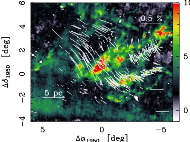
Fig. 2. Map of the cold dust emission in the Taurus molecular
com-plex built from the reprocessed 60µm and 100µm IRAS maps (Hily-Blant et al. 2007b) following the method of Abergel et al. (1995). The orientation of the projection of the magnetic fields on the sky (Heiles 2000) is shown as white segments of length proportional to the polar-ization degree. The parsec-scale field discussed in this paper is centered at α2000= 04h40m08.84s, δ2000= 24◦12
′ 48.40′′
and is shown as a white rectangle at offsets (0◦,-1◦).
these lines, Lis et al. (1996) have shown that it is possible to trace the projection of the most intense velocity-shears with a measurable quantity based on two-point statistics of the velocity field: the line centroid velocity increments (CVI). This method, applied to different fields observed in CO lines, a star-forming region (Lis et al. 1998) and quiescent regions (Pety & Falgarone 2003, hereafter PF03) revealed filamentary structures unrelated with the gas mass distribution. The line centroid velocities (and their increments) are sensitive to optical depth effects and to den-sity, temperature, and abundance fluctuations along the line of sight. Their relevance in any analysis of the statistical properties of the actual velocity fields have therefore been repeatedly ques-tioned. Several recent studies have clarified the issue (Lazarian & Pogosyan 2000; Miville-Deschˆenes et al. 2003; Levrier 2004; Ossenkopf et al. 2006) without having provided any final answer to that question yet. The present work is part of a broad study in which we characterize the structures of largest CVI on thermal, chemical, and statistical grounds, and then repeat this analysis in different turbulent clouds. The goal of this broad program is to shed light on what these structures actually trace.
One of the two fields studied in this paper is the parsec-scale environment of two low-mass dense cores in the Polaris Flare. In the vicinity of the dense cores, Falgarone et al. (2006) (hereafter Paper I) find HCO+abundances locally far in excess of steady-state chemical predictions. The large measured abundances are consistent with a scenario that involves an impulsive heating of the gas, during which a warm chemistry is triggered, followed by a slow chemical and thermal relaxation. According to this sce-nario, the observed abundances and gas densities, in the range 200 and 600 cm−3, correspond to a gas that has cooled down to 100–200 K. In Hily-Blant & Falgarone (2007a) (hereafter Paper II), we analyze the mass distribution of the gas in the envi-ronment of the dense cores and disclose localized regions where the12CO profiles exhibit broad wings. Multi-line analysis shows that gas in these linewings is optically thin in the12CO(1 − 0) line and warmer than 25 K with density < 1000 cm−3. The new
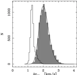
Fig. 3. Histograms of the equivalent width (∆veq=
R
T (vx) dvx/Tpeak) of the12CO(1 − 0) line in Polaris (shaded area) and Taurus. The result of the log-normal fit to the Polaris histogram is also shown.
result is that this warm gas component is not widespread but lo-calized in filaments. The dispersion of the orientation of the fila-ments of dense gas in the field, compared to the velocity disper-sion, suggests that the turbulence in that field is trans-Alfv´enic. In the forthcoming and last paper (Falgarone et al. 2008), we will report12CO(1 − 0) IRAM-Plateau de Bure observations per-formed in this field, revealing milliparsec-scale structures with large velocity-shears.
The present paper is dedicated to the statistical and struc-tural analysis of turbulence in similar parsec-scale translucent samples of gas, which belong to two different large-scale en-vironments: one, far from virial balance and devoid of stars, is the above-mentioned field in the Polaris Flare; the other lies at the edge of the Taurus-Auriga molecular complex. The statistical analysis is based on two-point statistics of the CO line emission observed at high spectral resolution, and the structural analysis consists in characterizing the regions of largest line-centroid ve-locity increments.
After presenting the data in Section 2, the characteristics of the turbulence in these two fields are derived based on the PDF of line CVI and structure functions (Section 3). We then show, in Section 4, that the regions of largest CVI on small-scales are fila-ments uncorrelated with the distribution of matter, but correlated with the filaments of gas optically thin in12CO(1−0) where large HCO+abundances are found. It is shown that these filaments re-main coherent at the parsec-scale. In Section 5, we show that the ensemble of results, based either on the statistical or structural approach, provides a consistent description of the intermittency of turbulence in these two fields. In Section 6, the comparison of the radiative cooling of these structures with the fraction of the turbulent energy susceptible to being dissipated there further supports the proposition that the filaments of largest CVI some-how trace extrema of velocity-shear in the fields and pinpoint the sites of intermittent dissipation of turbulence.
2. Observations
2.1. Polaris field
Paper II describes the observations and data reduction of the IRAM12CO and13CO(1 − 0) and (2 − 1) maps of the molecular cloud MCLD 123.5+24.9 located in the Polaris Flare. The
loca-Table 1. Dispersions σδC(in km s−1) of the PDF of CVI computed from
the12CO(1 − 0) transition in the Polaris and Taurus fields for different lags l (in pixels).
l σδC Polaris Taurus [pixels] [pc] km s−1 km s−1 3 0.02 0.11 0.05 6 0.05 0.17 0.07 9 0.07 0.22 0.09 12 0.09 0.25 0.10 15 0.11 0.27 0.11 18 0.14 0.29 0.12 18(a) 0.14 0.30 – 36(a) 0.27 0.46 – 54(a) 0.41 0.57 – 72(a) 0.54 0.64 – 90(a) 0.68 0.69 – 108(a) 0.81 0.72 –
(a) Computed from the KOSMA12CO(2 − 1) data of Bensch et al. (2001), where one
pixel corresponds to 6 pixels of the IRAM data. The adopted distance is 150 pc for both fields.
tion of the field mapped is shown in Fig. 1. The fully-sampled ≈ 1 pc×pc maps cover the non–star-forming translucent environ-ment of two dense cores (Gerin et al. 1997; Falgarone et al. 1998; Heithausen 2002), corresponding to ≈ 3000 independent spectra (i.e. spaced by one beamsize or 20′′
at 115 GHz). The spectral resolution is 0.055km s−1. Since the signal-to-noise ratio of the
J = 2−1 data is insufficient, only the J = 1−0 transition are used
in the present paper. For comparison with larger scale properties, we use the fully-sampled12CO(2 − 1) data from Bensch et al. (2001) obtained at a lower angular resolution (HPBW = 120′′
) with the 3m KOSMA antenna.
2.2. Taurus field
The second field is located at the edge of the Taurus-Auriga molecular complex (Fig. 2). Observations were done with the IRAM-30m telescope. Observational strategy and data reduction are similar to those of the Polaris field. The maps, centered at (α2000 = 04h40m08.84s, δ2000 = 24◦12
′
48.40′′
), are fully sam-pled in 12CO and 13CO(1 − 0). The data will be presented in more detail in a later paper (Hily-Blant & Falgarone 2008) but here we give the properties relevant to the present work. A total of 1200 independent spectra was obtained with the same spectral resolution of 0.055 km s−1. In a small region (around 0,0′′
offsets in the map of Fig. 9), spectra show two separate components (at
vLSR≈ 5 and 10 km s−1), and the analysis presented in this paper focuses on the main component at vLSR≈ 5 km s−1, by blanking out the area corresponding to the high-velocity component.
2.3. Comparison of the two fields
Both fields are translucent. The visual extinction lies between
AV = 0.6 and 0.8 mag at a resolution of 8′in the Polaris field (Cambr´esy et al. 2001) and between AV = 1 and 1.2 mag in the Taurus field at the same resolution (Cambr´esy 1999). As shown in Fig. 3, the most probable equivalent width (∆veq = R
T (vx) dvx/Tpeak, x being the coordinate along the line of sight)
of the12CO(1 − 0) line is a factor two larger in Polaris than in Taurus. However, since the lines are stronger in the Taurus field,
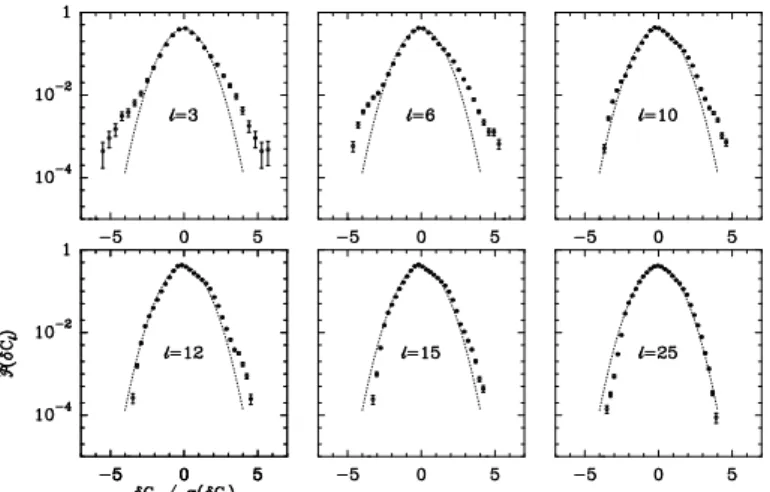
Fig. 4. Normalized PDF, Pn(δCl), of the centroid velocity increments (CVI) computed from the12CO(1 − 0) IRAM map in Polaris . The PDF are computed for different lags between pairs of points: l = 3 to 25 pixels, and normalized to unity dispersion, such that the x−axis is in units of the rms σδCfor each distribution. Only the bins containing more than 10 data points were kept. The values of the dispersion σδCare given in Table 1. A Gaussian of unit dispersion is also shown (dotted curve).
the integrated intensities in both fields are similar. Not only is the equivalent width larger in the Polaris field than in the Taurus one, but so is the dispersion of these equivalent widths. This factor 2 between the equivalent width translates into a factor 4 in the spe-cific kinetic energy ratio between the two fields. The distribution of the equivalent width in Polaris is also very well-fitted by a log-normal distribution centered at ∆veq = 2 km s−1with dispersion 1.2 km s−1. The parsec-scale velocity gradients, deduced from the centroid velocity maps, in the Polaris field (≈ 2 km s−1pc−1) is also twice larger than in the Taurus field.
These two parsec-scale fields are similar with respect to their size and average column density but have specific kinetic ener-gies that differ by a factor 4. Moreover, they belong to two very different environments on the scale of ∼ 30 pc, that of Figs. 1 and 2. The total gas mass Mtot= 4.4 × 10⁴M⊙at the scale of 30 pc is
close to the virial mass in the Taurus-Auriga field (Ungerechts & Thaddeus 1987), while it is more than six times lower in the Polaris Flare, Mtot = 5500 M⊙with Mv = 3.6 × 10⁴ M⊙
(Heithausen & Thaddeus 1990). It is interesting that the virial masses of the two large-scale fields are close, because their velocity dispersion on the scale of 30 pc are similar, 3.8 and 4.8 km s−1, respectively.
In summary, the less turbulent parsec-scale field lies on the far outskirts of the virialized Taurus-Auriga molecular complex, while the more turbulent field belongs to a much less massive complex, far from virial balance.
3. Two-point statistics of the centroid velocity
3.1. Probability density functions of the line centroid velocity increments
Following Lis et al. (1996), we analyze the two-point statistics of the centroid of the line-of-sight projection of the velocity vx,
which we note as C(y, z) = C(r), where (y, z) is the position on the sky: C(r) = Z T (r, vx)vxdvx/ Z T (r, vx) dvx. (1)
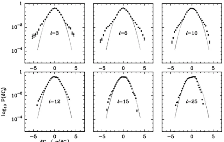
Fig. 5. Same as Fig. 4 for the12CO(1 − 0) data towards the Taurus field.
Increments of the centroid velocity between 2 points separated by l are defined by δC(r, l) = C(r + l) − C(r). This quantity will be called centroid velocity increment (CVI). The main difficulty of this method concerns the computation of C, which not only depends on the bounds of the integrals in Eq. 1, but is also af-fected by the signal-to-noise ratio (SNR). To circumvent the bias introduced by spatial noise variations, Rosolowsky et al. (1999) degrade all the spectra to a unique threshold SNR. A different approach (PF03) has been adopted here, which uses the SNR of the integrated area as the optimization criterion to determine the spectral window used to compute C. The reason is that we have checked that the noise is already homogeneous in the data cubes, mostly as a result of the observing strategy consisting in several coverages of individual sub-maps in perpendicular directions.
For a given value of l = |l|, we compute maps of CVI for each direction l/l. A probability density function (PDF) is built from these maps by normalizing the histogram of CVI to a unit area. We thus obtain a PDF for each l and each direction. For each l, a PDF is computed with the CVI from all directions l/l, which we denote as P(δCl). In order to get PDF with zero average and
unit standard deviation and to ease the comparisons, we use the normalized PDF Pn(δCl). All bins of the Pn(δCl) associated to
a number of points less than a given value Nminare blanked (see Appendix A.1). In the following, all Pn(δCl) have 32 bins, and
the adopted minimum number of data points for a bin to be sig-nificant is Nmin = 10. In a second step, for a given l, we compute the azimuthal average of the absolute value of the CVI, resulting in a single CVI map. In practice the structures seen in the non-averaged maps are not smeared out, though they appear thinner in some cases.
Figs. 4 and 5 show the Pn(δCl) computed for various lags
from l = 3 to 25 pixels in the Polaris and Taurus fields, respec-tively. The lag l = 3 is the shortest distance between two inde-pendent points (since the sampling is half the beam size), and
l = 25 corresponds to the largest lag with significant number of
pairs of points. The number of data points corresponding to the three most extreme bins for l = 3 and 25 are in the range 12 − 50 and 20 − 500, respectively.
The PDF at large lags (l > 15) (Fig. 4) are nearly Gaussian and become slightly asymmetrical at l = 12, an effect we at-tribute to large-scale velocity gradients. Such effects cancel out at lags smaller than the characteristic scale of these gradients, hence the more symmetrical shape of the PDF at small lags. It
Fig. 6. Same as Fig. 4 for the12CO(2 − 1) KOSMA data from Bensch et al. (2001).
is not obvious that such large-scale gradients should be removed (see discussion in PF03). The fields mapped here are expected to be small with respect to the integral scale of turbulence L, at least on the order of the molecular cloud size itself. As the lag de-creases from l = 25 to l = 3 pixels, non-Gaussian tails develop. These tails are more pronounced in the Polaris field than in the Taurus one, with CVI values up to 6 times the dispersions σδCof
the unnormalized PDF (see Table 1). However, since the number of points in Taurus is lower than in the Polaris field, the mini-mum level of probability reached is an order of magnitude higher (10−3instead of 10−4in Polaris). We also computed the PDF of the increments for the large-scale KOSMA data in the Polaris field (Fig. 6) and we also find increasing non-Gaussian tails as the lag decreases. The dispersions of the PDF are reported in Table 1 and are seen to smoothly connect with the small-scale values computed in the IRAM field.
In both fields, the dependence of σδCwith l can be well-fitted
by a power law σδC ∝ l0.5. The dispersions σδC in the Taurus
field are a factor ≈ 2 smaller than in the Polaris field. This ratio is also found when comparing the velocity dispersions – either across the plane of the sky (pos) or along the line of sight (los) – in the two fields (see Table 2). Furthermore, the ratio of the los to pos dispersions suggests that the depth of the cloud is larger than the extension in the plane of the sky (los > pos) (Ossenkopf & Mac Low 2002).
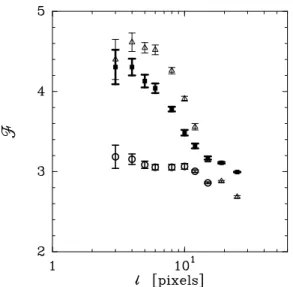
3.2. Non-Gaussianity: the flatness
The deviations of the PDF from a Gaussian shape can be quan-tified using the flatness (or kurtosis) of a distribution, defined by
F (l) = hδCl 4i hδCl2i2
(2) where the pth-order moment (for even p) is computed as hδClpi = R δClpPn(δCl) d(δCl). The flatness equals 3 for a
Gaussian distribution. The uncertainties, here and for all the mo-ments computed in what follows, are estimated by using two Pn(δCl) with two thresholds, Nmin= 1 and 10, and by computing
the mean and rms of the two outputs. Fig. 7 displays the flatness of the PDF at all lags, for the two fields. For the Polaris field, the IRAM and KOSMA data have a flatness close to 3 at large lags, which confirms the visual Gaussian shape of the corresponding
Table 2. Standard deviations σ (in km s−1) of the centroid velocity PDF
(pos) and of the average line profiles (los), computed in three ways in the two fields (σ1, σ2, σ3).
Field Type Size σ1 σ2 σ3 hσi
(1) (2) (3) (4) (5) (6) (7) Polaris† pos 2.1 × 2.8 0.54 0.57 0.60 0.57 ± 0.03 los 1.13 1.10 1.16 1.13 ± 0.03 Polaris‡ pos 0.7 × 0.6 0.31 0.32 0.25 0.29 ± 0.04 los 0.97 1.02 1.10 1.03 ± 0.05 Taurus‡ pos 0.4 × 0.7 0.12 0.13 0.11 0.12 ± 0.01 los 0.50 0.60 0.66 0.59 ± 0.07
(1) For the Polaris field, the IRAM (small) and KOSMA (large) datasets are taken sepa-rately. †: based on the12CO(2 − 1) data, ‡:12CO(1 − 0) data
(2) the type of PDF (pos or los)
(3) Map sizes (in pc × pc) are computed assuming a distance of 150 pc (4) σ1is the standard deviation
(5) σ2is derived from a Gaussian fit
(6) σ3= ∆veq/2.35
(7) average of the three determinations
PDF in Fig. 4. The flatness increases at smaller lags as a result of non-Gaussian tails. For the Taurus field, however, the flatness stays close to 3, confirming that the non-Gaussian tails are less pronounced.
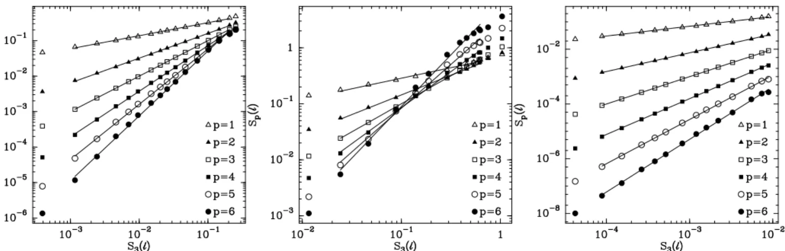
3.3. Structure functions of the line centroid velocities
By analogy with studies performed on the velocity field (e.g. She et al. 2001), we computed the structure functions of the line CV, using the PDF of the centroid velocity increments Pn(δCl),
a procedure that allows a check of the convergence of the struc-ture functions by filtering out doubtful points in the PDF. The structure functions are evaluated by a direct integration of the PDF:
Sp(l) =
Z ∞
0
|δCl|pPn(|δCl|) d(|δCl|). (3)
Structure functions of velocity are frequently normalized to the third-order function for two reasons: first because in incom-pressible, isotropic, and homogeneous turbulence, ζ(3) = 1 is an exact result; second because oscillations in Sp(l) − l plots are
damped when the Spare plotted against S3, a property called
ex-tended self-similarity (ESS) (Benzi et al. 1993), so that the range of scales over which the structure functions are power laws is wider.
Calculations of high-order structure functions are suscepti-ble to errors since, as p increases, any spurious large fluctuation largely affects Sp. The calculation of Spbased on Eq. 3 allows
us to reject bins populated by too small a number of points, and to study the influence of irrelevant bins of the PDF (for which
N < Nmin = 10). We also applied the procedure described in L´evˆeque & She (1997) and Padoan et al. (2003) for determining the highest significant order: the peak of the histogram of |δClp| occurs for a value of δClthat must be represented by a significant
number of points in the PDF of δCl. The maximum significant
order found is p = 6.
The scalings of Spwith S3are shown in Fig. 8 for the Polaris and Taurus fields. They are power laws. Exponents of the struc-ture functions are calculated by fitting the ESS diagrams for lags wider than 2 pixels and smaller than 30 to 60 (see Fig. 8). Error bars on the exponents (1 − 3%) are estimated from weighted averages of the results from two calculations corresponding to
Nmin=1 and 10. The ESS exponent values are given in Table 3. The absolute values of the second-order structure function in the
Fig. 7. Flatness F of the CVI (see Eq. 2) computed from the
normal-ized PDF of CVI. Squares: Polaris12CO(1 − 0) IRAM data. Triangles: 12CO(2 − 1) KOSMA data. Circles: Taurus12CO(1 − 0) IRAM data.
Taurus field are a factor 6 lower than in Polaris, confirming that the Taurus field contains less kinetic energy. The non-ESS fits of the CV structure functions lead to values for ζ(3) = 1.35 and 1.60 in Polaris and Taurus, which differ significantly from the expected value (ζ(3) = 1) for the velocity in incompressible, homogeneous, and isotropic turbulence (Kritsuk et al. 2007).
4. The spatial distribution of the largest line centroid velocity increments
In the following section, we discuss the spatial structures of the largest CVI in the different maps. We compare maps of CVI computed on large and small-scales with large and small beams. For the sake of simplicity, we call shear the CVI value divided by the lag over which it is measured, δCl/l. This will be justified
at the end of Section 5.
4.1. Locus of the extrema of CVI in the IRAM fields
Figs. 9 and A.3 show the maps of azimuthally averaged CVI (h|δCl|i) computed for two lags (l = 3 and 18 pixels) in both
fields. The grey scale is the magnitude of the azimuthally aver-aged CVI at a given position on the sky. Because of the averaging procedure, the exact values of the CVI in those maps are not triv-ially related to the values of the non-averaged PDF of Figs. 4 and 5. However, regions of large CVI in the maps do correspond to the positions responsible for the non-Gaussian tails in the PDF of Figs. 4-6.
At a small lag (l = 3), in both fields, the spatial distribution of the bright regions with large CVI delineates elongated structures. When the lag is larger (18 pixels), the contrast of the structures above the background values fades away. Yet, in the Polaris field, the structure around (−1000′′, −200′′) is still visible with l = 18,
and for the two lags of 3 and 18 pixels, the largest CVI is located in the northwestern corner of the map.
These maps show that the positions of the largest CVI, in Polaris and Taurus, are not randomly distributed but are con-nected and form elongated structures. In the Taurus field, the di-rection of the most prominent CVI structure is parallel to the projected orientation of magnetic fields measured in the NE
Table 3. Exponents ˜ζp= ζ(p)/ζ(3) of the ESS structure functions of the
CV for the Polaris and Taurus fields (see Fig. 14).
˜ζ1 ˜ζ2 ˜ζ3 ˜ζ4 ˜ζ5 ˜ζ6 Polaris 0.37 0.70 1.00 1.27 1.53 1.77 Polaris(a) 0.38 0.71 1.00 1.28 1.54 1.80 Taurus 0.36 0.69 1.00 1.30 1.60 1.89 SL94(b) 0.36 0.70 1.00 1.28 1.54 1.78 B02(b) 0.42 0.74 1.00 1.21 1.40 1.56
(a) From the large scale12CO(2 − 1) data from Bensch et al. (2001).
(b) SL94 and B02 are the She & L´evˆeque (1994) and Boldyrev et al. (2002) scalings of the velocity structure functions (see Section 5.2).
corner of the field (Heiles 2000) (see also Fig. 1). In Polaris, the scatter of their orientations relative to the magnetic field is larger (Paper II). In both Taurus and Polaris, their character-istic half-maximum width, measured on transverse cuts, is re-solved (30′′
after deconvolution from the lag, or d ≈ 0.02 pc), and their aspect ratio is often greater than 5. The surface frac-tions covered by the regions where the h|δCl|i are larger than
3σaver(where σaveris the dispersion of the distribution h|δCl|i),
are 10% and 28 % in Polaris and Taurus, respectively. Last, the non-averaged CVI in these structures (see Section 3.1) are 5 and 4 times larger than the dispersion σδC (see Figs. 4 and 5) in
Polaris and Taurus, respectively. For l = 3, the corresponding shears are 5 × 0.11 km s−1/0.02 pc = 30 km s−1pc−1in Polaris and 4 × 0.05 km s−1/0.02 pc = 10 km s−1pc−1in Taurus. The most turbulent field on the parsec-scale (Polaris) is therefore that where the largest small-scale shears are measured.
4.2. Comparison of the extrema of CVI with the CO emission We stress here that our work is based on the statistics of the extrema of CVI (called E-CVI in what follows), unlike what is done in most analyses (e.g. Esquivel & Lazarian 2005), where the full distribution of CVI is considered. We show below which specific features of the CO line emission are associated with the extrema of CVI.
Fig. 10 displays two12CO(1 − 0) space-velocity cuts made across the Polaris map at longitude offsets -500 and -800′′
. The run of the averaged CV and CVI along these cuts is shown to illustrate that the largest CVI are mostly due to very localized broad CO linewings. As expected, however, some of the large variations in the centroid velocities due to these broad wings are reduced by opposite variations due to fluctuations in the line-core emission.
This is seen better in Fig. 11 where the extrema of cen-troid velocity increments in the Polaris field are overplotted on the12CO wing emission and the13CO integrated emission. The 12CO wing emission (top panel) is optically thin and associ-ated with warm and tenuous gas emission (Paper II). The13 CO-integrated emission (bottom panel) is used here as a proxy for the molecular gas column density. While the largest CVI are not spa-tially correlated with the13CO-integrated emission, they closely follow the boundaries of the optically-thin12CO emission in the broad12CO linewings.
Given the high latitude of the Polaris cloud, the structures responsible for the broad12CO linewings most likely belong to the Polaris Flare (Fig. 1). The non-Gaussian tails of the PDF at small lags are thus associated to local structures on the scale of 30 pc. Their distance, and therefore their size, is known to
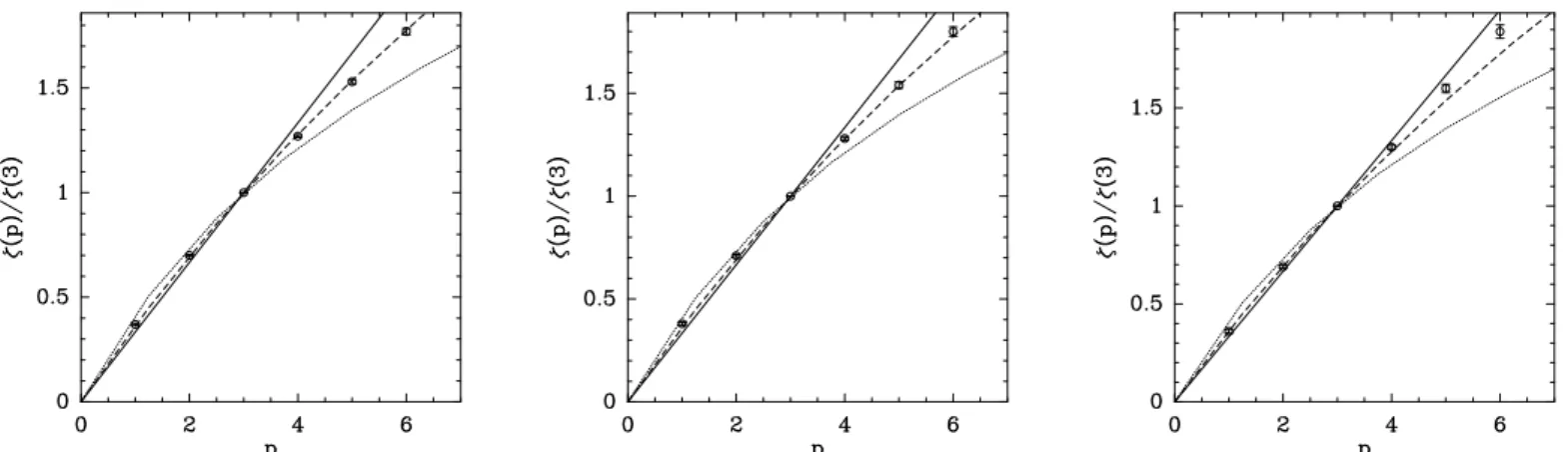
Fig. 8. Structure functions Sp(l) plotted against S3(l) (p = 1, . . . , 6) for Polaris (left for the IRAM data and middle for the KOSMA data) and Taurus (right). A power law is fitted to each order for l > 2 pixels, and for l < 60, l < 30, and l < 40 from left to right.
within 20%, while the lags of the PDF decrease by an order of magnitude (from 25 to 3). The l = 3 pixel PDF is thus sensitive to true small-scale structures created by the turbulence in the Polaris Flare. This comparison shows that the regions of largest shear are not associated with the bulk of the condensed matter in the field, but are instead correlated with warmer and more di-luted gas. We therefore infer that, unlike centroid velocities in-crements in general, the E-CVI we analyze are not due to density fluctuations or radiative transfer effects in optically thick gas.
We now address the issue of the chance coincidence of un-related pieces of gas on the line of sight. In the two translucent fields, CO is not expected to trace the full molecular content of the clouds, essentially as a result of photodissociation processes. This has possibly been observed by Sakamoto & Sunada (2003) who show discontinuous CO emission in low extinction regions in the Taurus complex. These spots of CO emission are how-ever embedded in the underlying turbulent molecular gas, un-detected because mostly made of molecular hydrogen, and pre-sumably continuous. The velocity field deduced from the CO emission lines thus carries the statistical properties of that turbu-lent molecular gas.
Nonetheless, projection effects are inevitable, and a key pa-rameter is the ratio l/L of the lag l over which CVI are measured to the unknown depth of the cloud along the line-of-sight L. In their work on 5123numerical simulations of mildly compress-ible turbulence, Lis et al. (1996) have computed PDF of CVI for a lag of 3 pixels, for which this ratio is 3/512=0.006. They show that the E-CVI trace extrema of h(∇ × v)yi2los+h(∇ × v)zi2los. Since
this quantity is a los integration of a signed quantity (the two projections of the vorticity in the plane of the sky), its extrema are due to a few exceptional values present on the line of sight. For this reason Lis et al. (1996) say that the E-CVI trace the pro-jection of large velocity-shears (or vorticity) in turbulence. In Polaris and Taurus, L is not known but we conservatively adopt a value in the range 1 − 30 pc. For the smallest lag (l = 3 pixels) the ratio is in the range l/L = 0.001 − 0.02. Our observational study thus falls into the regime tested by Lis et al. (1996), and the filaments associated with the E-CVI thus trace the projection of regions of extreme velocity-shear somewhere on the line of sight. The observed value of the shear, though, is of course an upper limit. We are therefore confident that E-CVI trace genuine extrema of line-of-sight velocity fluctuations.
4.3. Parsec-scale coherence of the regions of largest CVI: IRAM and KOSMA data
We compare here the properties of the E-CVI (values and spa-tial distribution) from the KOSMA and IRAM data sets of the Polaris field. The comparison is not, however, straightforward for two reasons. First, the value of the centroid velocity is af-fected by the beam size, and second, the computation of the CVI filters out any structures that are much larger than the lag.
Fig. 12 displays the spatial distribution of the CVI computed on large scales with the KOSMA data, for a lag l = 3 pixels (180′′). Regions of large increments are spatially resolved
fila-ments: cuts across the structures provide an average thickness of 200′′deconvolved from the lag, or 0.18 pc. These structures are
about 7 times thicker than those found in the IRAM field. The prominent KOSMA structure around (123.29◦, 25.11◦) smoothly connects with the northwestern IRAM structure (contours from Fig. 11). This is seen more clearly in Fig. 13 where the values of the non–averaged CVI along this structure are displayed. Fig. 13 illustrates three points: i) the CVI from the KOSMA and IRAM datasets decrease monotonously from north to south along this structure, ii) the IRAM CVI measured over l = 180′′
are all larger than those measured with KOSMA over the same physical lag, and iii) the CVI measured with the KOSMA telescope over a lag of 3 pixels (180′′
) are similar to those measured at the same po-sitions with the IRAM telescope with a lag 6 times smaller (30′′)
and .
The latter property is unexpected: it suggests that the CVI are similar in this region whether they are measured with a small beam and a small lag (IRAM) or a large beam and a large physi-cal lag. If the KOSMA structures were only due to beam-dilution of the IRAM ones, the KOSMA CVI for l = 180′′
would be smaller than the IRAM ones for l = 30′′. In other words, the
KOSMA CVI structures are real and are sub-structured: the same velocity variations (< 0.5 km s−1for positive offsets) are mea-sured on small (IRAM) and large (KOSMA) scales.
The largest velocity-shears at the KOSMA resolution are 5 × 0.30/0.18 ≈ 8.3 km s−1pc−1. The surface fraction covered by the large increment structures where h|δCl|i > 3σaverare close, 10 and 16% for the IRAM and KOSMA data, respectively. These two fields, observed with different telescopes and resolutions, thus show similar statistical properties and demonstrate the co-herence at the parsec-scale of the structures of largest centroid velocity increments. This is discussed in the next section.
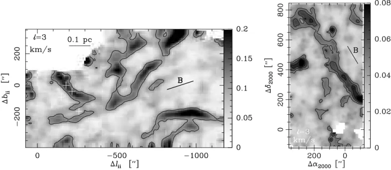
Fig. 9. Spatial distribution of the azimuthally averaged CVI (i.e. h|δCl|i) computed with lags l = 3 based on the12CO(1 − 0) line. The grey-scale gives the h|δCl|i in km s−1. The dark regions correspond to large values of the CVI associated to the tails of the P(δCl) (Fig. 4 and 5). The orientations of the magnetic fields (Heiles 2000) are also shown. Left panel: Polaris field. Contours indicate the 0.11 and 0.22 km s−1levels. The
largest CVI (0.30 km s−1) appear in the NW corner of the field. The 4 crosses indicate the positions where the HCO+abundances have been
measured (Paper I). Right panel: Taurus field. Map center is α2000= 04h40m08.84s, δ2000= 24◦12 ′
48.40′′
. Offsets are in′′
. Contours: 0.05 km s−1
with 0.01 km s−1steps. Note that the largest CVI (0.10 km s−1) in that field are 3 times smaller than in the Polaris field. The blanked areas around
(0, 0) offsets correspond to the positions where the 10 km s−1component is present.
5. The two facets of intermittency: statistical and structural
In Section 3, the two-point statistics of the line centroid ve-locities were found to display marked non-Gaussian behaviors. In Section 4, the emission responsible for these non-Gaussian statistics is resolved into coherent structures. We here compare these statistical and structural characteristics with theoretical predictions and recent numerical results regarding the intermit-tency of turbulence.
5.1. Self-similarity of the centroid velocity increments in the Polaris field
The IRAM and KOSMA PDF from Figs. 4 and 6 bear an appar-ent contradiction: the PDF built with the IRAM data with a lag of 150′′
(15 pixels) is nearly Gaussian, while the KOSMA PDF with a similar physical lag of 180′′(3 pixels) is not: non-Gaussian tails
in the KOSMA PDF originate from the largest CVI structures like the most prominent one discussed in Section 4.3. In Fig. 13, we show that the bulk of the IRAM CVI for l = 180′′
(dark dots) are below 3σδC = 0.9km s−1. It is the particular location
of the IRAM field with respect to the CVI maxima seen in the KOSMA field that prevents the detection of a number of CVI in excess of 3σδC large enough to depart from Gaussian statistics.
Would the IRAM field be centered closer to the CVI maximum in the KOSMA data (around 123.29◦, 25.11◦), a larger number of CVI in excess of 3σδCmight have been measured.
However, in both fields, the non-Gaussian tails of the PDF of CVI grow as the lag decreases. This behavior is routinely observed in laboratory and numerical experiments, where it is interpreted as a signature of the intermittency of the velocity field. In such experiments, effects of the non-Gaussian statistics are visible with either the transverse or the longitudinal
veloc-ity increments (Frisch 1995; Mininni et al. 2006a). The present analysis shows various degrees of non-Gaussianity: the statistics in Taurus are nearly Gaussian (flatness close to 3), while both Polaris data sets show clear departure from Gaussianity. If, fol-lowing PF03, we attribute the non-Gaussian statistics of the CVI to the intermittency of the turbulence in the two sampled molecu-lar clouds (see below), the new result, here, is that intermittency is as pronounced at a lag l = 180′′in the large field (KOSMA
PDF) as it is at lag l = 30′′
in the IRAM field. In both datasets, the non-Gaussian tails extend to 5.5 − 6σδC. This suggests that
intermittency is not only a small-scale phenomenon but that it is present and has the same statistical properties on a scale six times larger.
As mentioned in the introduction, similar conclusions have been reached by MJ04, who find that the intense structures of vorticity and rate of strain in hydrodynamical turbulence form clusters of inertial range extent, implying a large-scale organiza-tion of the small-scale intermittent structures.
5.2. The intensity of small-scale intermittency versus large-scale shear
We now compare the scaling of the pth-order structure functions of CV with p in the framework of the SL94 model. Structure functions are increasingly sensitive to the tails of the CVI PDF (E-CVI) as the order p increases. Since we have shown (Sect 4.2) that the E-CVI stem from velocity fluctuations, it is interesting to compare the scaling of high order structure functions of the CV to theoretical predictions based on the velocity field.
The SL94 model has three parameters (see Appendix A.3). One of the three parameters, 0 ≤ β ≤ 1, describes the level of intermittency: β → 1 corresponds to the non-intermittent cas-cade with ˜ζp = p/3. The two other parameters (Boldyrev et al.
Fig. 10. Position-velocity cuts at constant ℓIIoffsets (∆ℓII=−500′′, left and ∆ℓII=−800′′
, right). Grey-scale: main-beam intensity in K. Dashed curve: centroid velocity. Full curve: azimuthally averaged CVI for a lag l = 3 pixels (with an additional offset of -6.5 km s−1for clarity).
2002) describe the scalings of velocity in the cascade and the dimension D of the most intermittent structures. In the SL94 model, the scaling of the velocity is vl ∼ l1/3. It assumes that
the most intermittent structures are filaments (D = 1) and that the level of intermittency is β = 2/3. The associated ESS struc-ture function exponents ˜ζp = ζ(p)/ζ(3) are then predicted to
be ˜ζSL
p = p/9 + 2[1 − (2/3)p/3]. According to this class of
models, as the level of intermittency increases, the ESS expo-nents become smaller than p/3 for p > 3 and the departure from the K41 scaling increases with p. Following the SL94 approach, further theoretical models were developed for com-pressible and magnetized turbulence (Politano & Pouquet 1995; M¨uller & Biskamp 2000) and tested against numerical simula-tions. Boldyrev et al. (2002) propose a similar scaling to de-scribe compressible MHD turbulence assuming sheet-like in-termittent structures (D = 2) and a more inin-termittent cascade (β = 1/3) but do not allow dissipation of large-scale modes in shocks. They find ˜ζB02
p = p/9 + 1 − (1/3)p/3(hereafter called the
B02 scaling), in excellent agreement with numerical simulations of super-Alfv´enic MHD turbulence. However, this scaling has never been tested against observations of the turbulent velocity field of molecular clouds.
In Fig. 14, we compare the scalings of the CV structure func-tions exponents (see Table 3) with the predicfunc-tions of the SL94 and B02 models for the velocity field. In the Polaris field, for either data set, the measured exponents follow the SL94 scaling closely but differ significantly from that of B02. This apparent agreement with the SL94 scaling is unexpected since this model describes incompressible and unmagnetized turbulence, every-thing interstellar turbulence is not. However, the effect of line-of-sight averaging in the CV structure functions is not known. Further interpretation of the underlying physics requires con-frontation with CV structure functions based on numerical sim-ulations. The exponents in the Taurus field do not follow any of the three scalings, and are halfway between the non-intermittent K41 scaling ( ˜ζ(p) = p/3) and the SL94 scaling. The Taurus field is thus less intermittent than the Polaris one, a result consistent with the flatness measure of the non-Gaussianity of the P(δCl).
This result is also in line with the recent numerical findings of Mininni et al. (2006a), who show that the characteristics of the large-scale flow play an important role in the development of small-scale intermittency and determine its statistical properties. The use of CV structure functions to determine the three pa-rameters of the SL94 class of models not only requires a large number of data points but also “calibration” of the weighting
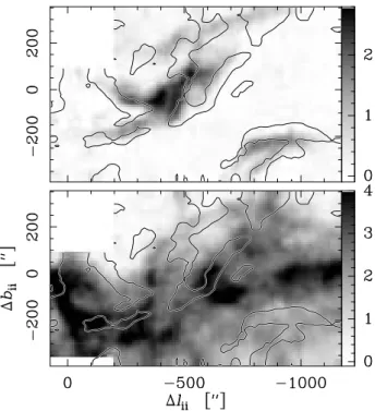
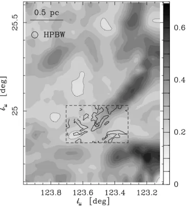
Fig. 11. Contours of the CVI (1 km s−1) computed in the Polaris field
for l = 3 pixels (see Fig. 9) overplotted on the12CO(1 − 0) emission integrated in the velocity range [−2, 5 : 0] km s−1 i.e. optically thin
12CO emission (top) and the13CO integrated intensity tracing the bulk of the dense gas (see Paper II) (bottom).
performed by CV upon the velocity field, using numerical simu-lations of compressible turbulence. The values that we have de-termined from the exponents ˜ζ(p) may be useful, though, and we give them in the Appendix.
In summary, the line CV exhibit the statistical and structural properties characterizing the intermittency of the velocity field in theoretical models and numerical simulations of turbulence: 1) the non-Gaussian statistics of the CVI at small lag, 2) the self-similarity of structures of largest CVI and the existence of inertial-range intermittency, 3) the anomalous scaling of their high-order structure functions similar to wthat is found for the structure functions of velocity. Last, we find that the more in-termittent field on small scales has the larger dispersion of non-thermal velocity on large scales.
The above properties are borne by the non-Gaussian tail of the CVI PDF, which we have shown to be associated with pure velocity fluctuations. They support our proposition that statis-tics of the 12CO line centroid velocity and, more specifically, their E-CVI may be used to disclose the statistical and structural properties of intermittency in the underlying velocity field. In what follows, we therefore ascribe the E-CVI to the intermittent structures of intense shears.
6. Discussion
6.1. Influence of gravity
To test the role of gravity in the generation of non-Gaussian statistics of the velocity, Klessen (2000) built the two-point statistics of the velocity field, in SPH numerical simulations of turbulence, both with and without self-gravity . The author com-pared the numerical PDF of CVI with observed PDF and con-cluded that the inclusion of self-gravity leads to better agree-ment with the observed PDF in molecular clouds. It was
fur-Fig. 12. Spatial distribution of CVI (km s−1) computed on large scales
using the data of Bensch et al. (2001) (grey-scale with levels indicated on the right scale, dotted contours indicate the 0.1 km s−1 level).
Full-line contours indicate the CVI computed on small scales in the IRAM-30m data cube (see Fig. 11). Note the spatial coincidence of the IRAM structures at the tip of the prominent KOSMA structure at (123.4◦, 25◦),
where the CVI are 0.30 km s−1.
ther argued in PF03 that this result was indeed expected since the observed regions used in the comparison are forming stars, hence the importance of self-gravity. The situation is drastically changed in the two translucent fields we have studied: they do not form stars, are far from any such regions, and both are non– self-gravitating on the parsec-scale of our observations. Indeed, we have shown that the field with the more prominent non-Gaussian tails, namely Polaris, is located at high latitude and is embedded in a larger structure (the Flare) far from virial bal-ance. This strongly supports that, in the type of fields we analyze, gravity is not at the origin of the PDF tails.
Nonetheless, gravity is the ultimate source of gas motions in the universe, from galaxy clusters to GMC and collapsing cores, so it cannot be ignored. If the cloud mass were distributed in tiny cloudlets of very high density that would rarely collide, then gravity might play a significant role in the gas velocity statis-tics. Here, we assume that the fluid approximation is valid, and because the Reynolds number is so large, the gas motions are turbulent, by definition.
6.2. The intermittency of turbulence dissipation
In numerical experiments such as those of MJ04 (see also Sreenivasan 1999), maxima of energy dissipation are found, at small-scale, in the vicinity of the vorticity filaments. A large fraction of the dissipation of turbulence may be concentrated in the regions of largest CVI, the small-scale intermittent struc-tures. We illustrate this point with estimates of energy transfer based on our observations in the Polaris field.
Fig. 13. Values of the CVI in the Polaris field, along the NW-SE CVI
structure from (123.2, 25.2◦) to (123.6, 24.9◦) seen in Fig 12. CVI are
from KOSMA data for l = 3 (diamonds), IRAM l = 3 (open circles), and IRAM l = 18 (filled circles). Offsets increase from NW to SE, with the zero position corresponding to the NW corner of the IRAM field (see Fig. A.2).
The transfer rate in the cascade on scale l is ǫl = 1/2ρv3l/l
with vl the characteristic turbulent velocity fluctuations on that
scale. This assumes that the time to transfer energy from scale l to smaller scales writes as τl = l/vl. At the parsec-scale of the
Polaris cloud
ǫL= 5.5×10⁻²⁵/L2pc erg s−1cm−3 (4) where the average density ρ = µNH/L and the velocity
disper-sion vL = 1.5 km s−1are those derived in Paper II. There, Lpcis
the unknown depth along the line of sight, expressed in pc. The CO cooling rate averaged over the whole field on the parsec-scale is (Paper II)
ΛCO= 10−24/Lpc erg s−1cm−3. (5)
These two rates are thus close, because the depth along the line of sight is not much greater than 1 pc (see Section 3.1), and may lead to the conclusion that CO is able to radiate the turbulent en-ergy away, confirming the results of Shore et al. (2006). Actually, this would be true if the cascade were filling space uniformly or, in other words, for a non-intermittent cascade. From the previ-ous section, this assumption is certainly not valid. Indeed, the cumulative distribution of δC2
l for l = 3 (see Fig.B.1) shows that
the points with CVI larger than 3σδCrepresent only 2.5% of the
total, while they contribute to 25% of the total of δC2
l. The
ve-locity field has two contributions (solenoidal and dilatational) to the energy dissipation rate ǫ = −Re1 (|∇ × v|2+43|∇ · v|2) (Kritsuk et al. 2007). As shown by Lis et al. (1996) and Pety & Falgarone (2000) based on numerical simulations, the E-CVI serve as a proxy for large vorticity regions. Thus, assuming that the energy dissipation on scale l is proportional to δC2l, the cumulative dis-tribution of Fig. B.1 suggests that the local dissipation rate at
l = 3 (or ∼ 0.02 pc) in the E-CVI regions, is already 10 times
larger than the average rate over the field, ǫE−CVI >10ǫL. Note
that these numbers are about the same for the large-scale Polaris field, while in the less intermittent Taurus field, these E-CVI rep-resent only 1% of the total, still contributing to 5% of the dissi-pation.
Fig. 14. Values of the exponents of the structure functions (see Fig. 8) with error bars (see Table 3). For comparison, the K41 (full), SL94 (dashed),
and B02 (dotted) scalings are indicated. From left to right: Polaris (IRAM), Polaris (KOSMA), Taurus.
On the actual dissipation scale, presumably smaller than 0.02 pc, the local dissipation rate is still higher by an unknown factor. Since the turbulent dissipation is not space-filling, it in-duces high local heating rates. This suggests that other cool-ing agents, e.g. the pure rotational lines of H2 or the fine struc-ture line of C+, may be dominating the cooling in these regions (Paper I and Falgarone et al. 2007). Observations are still lack-ing that would allow a comparison of the turbulent transfer rate with the CO cooling rate on scales smaller than 0.02 pc.
In spite of the self-similarity of the intermittent structures discussed in Section 5, the bulk of the dissipation is likely to take place in the smallest structures. The largest CVI are propor-tional to σδC and thus to l1/2. The corresponding shears
there-fore scale as l−1/2providing an observed scaling of the dissipa-tion rate with lengthscale l, ǫl ∝ l−1. Now, we use the finding
of MJ04, who show that the tails of the probability distribution functions of the volume of individual dissipative structures (ei-ther intense vorticity or strain-rate) decrease approximately as
p(V) ∼ V−2. Whether these structures are cylinders (V ∝ l2) or sheets (V ∝ l), the integrated dissipation is therefore always dominated by the dissipation which takes place on the smallest scales, because p(V)ǫl∝ l−5in the first case or ∝ l−3in the
sec-ond case.
This confirms the important point for the evolution of molec-ular clouds that dissipation of turbulence is concentrated in a small subset of space. The induced radiative cooling, and there-fore the dissipation rate, have to be searched on scales on the or-der of the milliparsec in emission lines more powerful than the low−J CO transitions. The value of the rate itself may thus be directly observable in line emissions (pure rotational lines of H2, C+) that can only be distinguished from UV-excited emission by observations at very high angular resolution.
7. Conclusion and perspectives
We performed a statistical analysis of the turbulence towards two translucent molecular clouds based on the two-point probability density functions of the12CO(1 − 0) line centroid velocity.
Thanks to the excellent quality of the data, we prove the non-Gaussian tails in the PDF of the line centroid velocity increments on small-scales, down to a probability level of 10−4. We show that the largest CVI, in both fields, delineate elongated narrow structures (∼ 0.02 pc) that are, in one case, parallel to the local direction of the magnetic field. In the Polaris field, these fila-ments are well-correlated to the warm gas traced by the optically
thin12CO(1−0), while they do not follow the distribution of mat-ter traced by the13CO. Using large-scale data, we have shown that these filamentary structures remain coherent over more than a parsec. Furthermore, the similar statistics found in the IRAM and KOSMA maps of this field suggest that both samples be-long to the self-similar turbulent cascade. In the Polaris field, the high-order structure function exponents, computed up to order
p = 6, significantly depart from their Kolmogorov value.
Through the properties of the tails of their PDF, i.e. the E-CVI, the line centroid velocities in these two clouds are found to carry the main signatures of intermittency borne by a turbu-lent velocity field. The departure from the Gaussian statistics of the centroid velocity increments on small-scales is therefore as-cribed to the intermittency of turbulence, i.e. the non-space fill-ing character of the turbulent cascade. The structures of largest CVI trace the intermittent structures of intense shears and the sites of intermittent turbulence dissipation. We show that these intermittent structures, on the 0.02 pc-scale, harbour 25% and 5% of the total energy dissipation, in the Polaris and Taurus fields, respectively, although they fill less than 2.5% and 1% of the cloud area. We find that both fields are intermittent and that the more intermittent velocity field on small scales (the Polaris field) belongs to a molecular cloud far from virial balance on the scale of 30 pc. In contrast, the less intermittent (the Taurus field) belongs to a virialized complex. The more turbulent field is thus the more intermittent. Interestingly enough, the less turbu-lent field is embedded in a star-forming cloud (Taurus complex) with numerous young stellar objects, while the more turbulent (Polaris) is in an inactive complex.
The exact nature of these intermittent structures, their link with shocks, and the role of magnetic fields are still elusive. The comparison of observational data with theoretical scalings re-quires the ability to compute higher orders of the structure func-tions and establish the correspondence between the centroid ve-locity and the veve-locity fields. This stresses the need for large homogeneous data samples with at least 105spectra. Such data sets would also allow determination of the three parameters of the class of models to which the SL94 or MHD scalings belong. Heterodyne instrumentation (e.g. multi-beam receiver het-erodyne arrays) offers a dramatic increase in the spatial dynam-ical range accessible, combining high spatial and spectral reso-lutions. Sub-arcsecond resolution is needed to resolve the dissi-pation scale, combined with a large instantaneous field of view to disclose the shape of the dissipative structures. Observational signatures of the dissipation of the turbulent kinetic energy might
be searched for in chemical abundances of species, whose for-mation requires high temperatures (Paper I), like CH+, HCO+, and water. Excited H2was also proposed as a good coolant can-didate (Falgarone et al. 2005; Appleton et al. 2006). While some of these observational requirements are already met by existing instruments (e.g. HERA at the IRAM-30m telescope), ALMA, SOFIA, and the Herschel satellite will definitely open new per-spectives in this field.
Acknowledgements. We thank the anonymous referee for his careful reading of the manuscript and useful comments that helped us to improve the paper. EF and PHB acknowledge the hospitality of the Kavli Institute for Theoretical Physics (Grant No. PHY05-51164) during the revision phase of their manuscript. The au-thors also thank A. Lazarian for useful comments and M.-A. Miville-Deschˆenes for providing them with the IRIS maps of Fig. 1.
References
Abergel, A., Boulanger, F., Fukui, Y., & Mizuno, A. 1995, A&AS, 111, 483 Anselmet, F., Antonia, R. A., & Danaila, L. 2001, Planet. Space Sci., 49, 1177 Anselmet, F., Gagne, Y., Hopfinger, E. J., & Antonia, R. A. 1984, J. Fluid Mech.,
140, 63
Appleton, P. N., Xu, K. C., Reach, W., et al. 2006, ApJ, 639, L51 Bate, M. R., Bonnell, I. A., & Bromm, V. 2002, MNRAS, 332, L65 Bensch, F., Stutzki, J., & Ossenkopf, V. 2001, A&A, 366, 636 Benzi, R., Ciliberto, S., Tripiccione, R., et al. 1993, Phys. Rev. D, 48, 29 Boldyrev, S., Nordlund, Å., & Padoan, P. 2002, Phys. Rev. L., 89, 031102 Bruno, R. & Carbone, V. 2005, Living Rev. Solar Phys., 2
Cambr´esy, L. 1999, A&A, 345, 965
Cambr´esy, L., Boulanger, F., Lagache, G., & Stepnik, B. 2001, A&A, 375, 999 Ciolek, G. E. & Basu, S. 2006, ApJ, 652, 442
Crutcher, R. M. 1999, ApJ, 520, 706
Crutcher, R. M. 2005, in AIP Conf. Proc. 784: Magnetic Fields in the Universe: From Laboratory and Stars to Primordial Structures., ed. E. M. de Gouveia dal Pino, G. Lugones, & A. Lazarian, 129–139
Douady, S., Couder, Y., & Brachet, M. E. 1991, Phys. Rev. L., 67, 983 Elmegreen, B. G. & Scalo, J. 2004, Annual Review of Astronomy and
Astrophysics, 42, 211
Esquivel, A. & Lazarian, A. 2005, ApJ, 631, 320
Falgarone, E., Hily-Blant, P., Pety, J., & Pineau Des Forˆets, G. 2007, in IAU Symposium, Vol. 237, IAU Symposium, ed. B. G. Elmegreen & J. Palous, 24–30
Falgarone, E., Panis, J.-F., Heithausen, A., et al. 1998, A&A, 331, 669 Falgarone, E., Pety, J., & Hily-Blant, P. 2008, in prep.
Falgarone, E., Pineau Des Forˆets, G., Hily-Blant, P., & Schilke, P. 2006, A&A, 452, 511
Falgarone, E., Verstraete, L., Pineau Des Forˆets, G., & Hily-Blant, P. 2005, A&A, 433, 997
Frisch, U. 1995, Turbulence. The legacy of A.N. Kolmogorov (Cambridge University Press)
Gerin, M., Falgarone, E., Joulain, K., et al. 1997, A&A, 318, 579 Heiles, C. 2000, Astron.J., 119, 923
Heithausen, A. 2002, A&A, 393, L41
Heithausen, A. & Thaddeus, P. 1990, ApJ, 353, L49 Hily-Blant, P. & Falgarone, E. 2007a, A&A, 469, 173 Hily-Blant, P. & Falgarone, E. 2008, in prep.
Hily-Blant, P., Pety, J., & Falgarone, E. 2007b, in Astronomical Society of the Pacific Conference Series, Vol. 365, SINS - Small Ionized and Neutral Structures in the Diffuse Interstellar Medium, ed. M. Haverkorn & W. M. Goss, 184–+
Klessen, R. S. 2000, ApJ, 535, 869 Klessen, R. S. 2001, ApJ, 556, 837
Kritsuk, A. G., Norman, M. L., Padoan, P., & Wagner, R. 2007, ApJ, 665, 416 Lazarian, A. & Pogosyan, D. 2000, ApJ, 537, 720
Lesieur, M. 1997, Fluid Mechanics and its Applications, Vol. 40, Turbulence in Fluids, 3rd edn. (Dordrecht, Netherlands: Kluwer)
L´evˆeque, E. & She, Z.-S. 1997, Phys. Rev. D, 55, 2789 Levrier, F. 2004, A&A, 421, 387
Lis, D. C., Keene, J., Li, Y., Phillips, T. G., & Pety, J. 1998, ApJ, 504, 889 Lis, D. C., Pety, J., Phillips, T. G., & Falgarone, E. 1996, ApJ, 463, 623 Mac Low, M. & Klessen, R. S. 2004, Rev. Mod. Phy., 76, 125 Matthews, B. C. & Wilson, C. D. 2000, ApJ, 531, 868
Mininni, P. D., Alexakis, A., & Pouquet, A. 2006a, Phys. Rev. D, 74, 016303 Mininni, P. D., Pouquet, A. G., & Montgomery, D. C. 2006b, Phys. Rev. L., 97,
244503
Miville-Deschˆenes, M.-A., Levrier, F., & Falgarone, E. 2003, ApJ, 593, 831 Miville-Deschˆenes, M.-A. & Lagache, G. 2005, Ap. J. Supp., 157, 302 Moisy, F. & Jim´enez, J. 2004, J. Fluid Mech., 513, 111
M¨uller, W.-C. & Biskamp, D. 2000, Phys. Rev. L., 84, 475
Ossenkopf, V., Esquivel, A., Lazarian, A., & Stutzki, J. 2006, A&A, 452, 223 Ossenkopf, V. & Mac Low, M.-M. 2002, A&A, 390, 307
Padoan, P., Boldyrev, S., Langer, W., & Nordlund, Å. 2003, ApJ, 583, 308 Padoan, P., Juvela, M., Goodman, A. A., & Nordlund, Å. 2001, ApJ, 553, 227 Pety, J. & Falgarone, E. 2000, A&A, 356, 279
Pety, J. & Falgarone, E. 2003, A&A, 412, 417 Politano, H. & Pouquet, A. 1995, Phys. Rev. D, 52, 636
Porter, D. H., Pouquet, A., & Woodward, P. R. 1994, Phys. Fluids, 6, 2133 Rosolowsky, E. W., Goodman, A. A., Wilner, D. J., & Williams, J. P. 1999, ApJ,
524, 887
Sakamoto, S. & Sunada, K. 2003, ApJ, 594, 340 She, Z.-S. & L´evˆeque, E. 1994, Phys. Rev. L., 72, 336
She, Z.-S., Ren, K., Lewis, G. S., & Swinney, H. L. 2001, Phys. Rev. D, 64, 016308
Shore, S. N., Larosa, T. N., Chastain, R. J., & Magnani, L. 2006, A&A, 457, 197 Sreenivasan, K. R. 1999, Rev. Mod. Phy., 71, S383
Tassis, K. & Mouschovias, T. C. 2004, ApJ, 616, 283 Ungerechts, H. & Thaddeus, P. 1987, Ap. J. Supp., 63, 645 Vincent, A. & Meneguzzi, M. 1991, J. Fluid Mech., 225, 1
Appendix A: Two-point statistics
A.1. Construction of thePn(δCl)
In each PDF, all the bins which are associated to a number of events less than a given value Nmin, are blanked. The value of Nmindepends on the number of bins in the histogram. In Fig. A.1, we show the Pn(δCl) computed for l = 3 in
the Polaris field, for successive values of Nmin=0, 10, 30, and 100. It is seen that, with Nmin=10, the spurious bins having a constant value ≈ 10−4are eliminated. The value of each bin and its uncertainty are then determined from the average and rms of all the points populating the bin.
A.2. CVI maps
The non-averaged CVI map of Fig. A.2, computed in the IRAM data for a lag of 18 pixels (or 180′′
), shows that large-scale structures exist that are not filtered out with large enough lags. The crosses indicate the positions where the CVI values of Fig. 13 have been taken.
Figure A.3 shows the CVI map computed in the IRAM Polaris and Taurus fields, for a lag of 18 pixels. The comparison with the CVI maps of Fig. 9 shows that the thin filaments have faded away. However, in the Polaris map, the struc-ture visible at a lag of 3 pixels is still visible, though it has broadened.
A.3. Determination of the intermittency level
She & L´evˆeque (1994) developed a model to analyze the small-scale properties of an incompressible turbulent flow. Since this model inspired numerous works of astrophysical relevance, we summarize its key points here. SL94 propose studying the large fluctuations of ǫl(defined as the dissipation rate averaged over
balls of size l) through the ratio of its successive moments ǫl(p) =hǫlp+1i/hǫlpi.
Hence, for each p, the value of ǫl(p)describes the dissipation intensity of a set of turbulent structures: as p increases, the associated structures are more coherent and more singular. As a result, the hierarchical structures of the SL94 model are not related to any physical objects, except for the most intermittent. The SL94 model has three parameters: the scaling of the velocity with scale l, assumed to be that of the K41 theory (vl ∼ l1/3); the level of intermittency characterized
by a parameter β; and the dimensionality D of the most intermittent structures. Assuming β = 2/3 and D = 1, SL94 proposed a recursive relation linking ǫl(p+1) to ǫl(p),
ǫl(p+1)= Apǫl(p)
β
ǫ(∞)l 1−β, (A.1)
which allowed them to compute the anomalous scaling of the energy dissipation rate with scale l, hǫlpi ∼ lτp, with τ
p=−2/3p + 2[1 − (23)p].
In principle, by fitting the exponents ˜ζ(p), it should be possible to determine the three parameters of the SL94 class of models. In practice, a reliable determi-nation of the three parameters, e.g. by least-square fitting the exponent values, requires computing high-order structure functions (p > 6). With 6 orders, we could only determine one parameter, the scaling of the velocity fluctuations in the cascade vl∝ lθand we found θ = 1/3 which coincides with the K41 value.