Assessing the Hydrocarbon Emissions in a Homogeneous Direct
Injection Spark Ignited Engine
by
Michael S. Radovanovic
B.S., Mechanical Engineering Purdue University, 2004
SUBMITTED TO THE DEPARTMENT OF MECHANICAL ENGINEERING IN
PARTIAL FULFULLMENT OF THE REQUIREMENTS FOR THE DEGREE OF
MASTER OF SCIENCE IN MECHANICAL ENGINEERING
AT THE
MASSACHUSETTS INSTITUTE OF TECHNOLOGY
August 2006
0 2006 Massachusetts Institute of Technology All Rights Reserved
Signature of Author:
Department of Mechanical Engineering August 11, 2006 Certified by:
Wai K. Cheng Professor of Mechanical Engineering Thesis Supervisor Accepted by:
Lallit Anand Chairman, Departmental Graduate Committee
MASSACHUSETTS IN$T1IUTE.
OF TECHNOLOGY
Assessing the Hydrocarbon Emissions in a Homogeneous Direct
Injection Spark Ignited Engine
By
Michael S. Radovanovic
Submitted to the Department of Mechanical Engineering On August 11, 2006 in Partial Fulfillment of the Requirements for the Degree of Masters of Science in
Mechanical Engineering
Abstract
For the purpose of researching hydrocarbon (HC) emissions in a direct-injection spark ignited (DISI) engine, five experiments were performed. These experiments clarified the role of coolant temperature, injection pressure, and injection timing in HC emissions; the
final two experiments illustrated the effect of coolant temperature and injection pressure on separate sweeps of injection timing and the subsequent HC levels. The first three
experiments were performed with isopentane. All five of the experiments were repeated with two fuels: UTG 91, a typical research gasoline, and a fuel with a high driveability
index (DI), i.e. a less volatile fuel.
The results showed less-than intuitive results for the response of HC to varying coolant temperature and varying injection pressure. For the coolant temperature data, the deviation
from intuition is discussed and is probably due to vaporization problems. For the injection pressure results, the counterintuitive trend is expected to be the balance of two negative
effects of high and low fuel pressure: high droplet velocities and large droplet diameters. Finally, the injection timing results were more logical. The early injections are high for this
engine due to late exhaust valve closing, and the late injections have high HC because of a decreasing time to vaporize and poor mixing caused by the lack of intake air motion. Thesis Supervisor: Wai K. Cheng
Acknowledgements
For the opportunity to learn at MIT, I'm thankful to the group of automotive and oil companies which funded my research and education. Raymond Phan and Thane DeWitt, on staff at the lab, were critical to setting up my project; without them, I could not have completed my project. In particular, I am appreciative of Professor Cheng. The last month has included enjoyable and humorous moments as we attempted to combine our intellects and understanding to explain the data. "Before you leave MIT you'll learn that everything is rational," as he rapped a check valve with a wrench to fix my fuel supply problem.
I have made good friends in the lab and having this close-knit group of people made my
stay at MIT more bearable. Vince Costanzo, Alex Sappok, and Kevin Lang provided especially amiable company. Developing black and white photos in the SAA and making projects in Hobby Shop were wonderful outlets for me, and they played an important role in several pleasant memories at MIT.
Even more critical to my state-of-mind has been the support, prayers and social interaction I've received from numerous people from Hope Fellowship Church. I've yet to meet a group of people who care so much for the well-being of others, for their temporary needs and their eternal ones. Leaving this community will definitely be the hardest part about leaving Boston. "And now, 0 Israel, what does the Lord your God ask of you but to fear the Lord your God, to walk in all his ways, to love him, to serve the Lord your God with all your heart and with all your soul, and to observe the Lord's commands..." Deuteronomy
10: 12-13a.
A few friends deserve special mention: Clay Edens, for weekly conversations, Jeffrey D.
Robinson, for funny voicemail messages, Chris Sullivan, for sharing food and guitar interests, Randy Ewoldt, for tremendously enjoyable lunches, and Mila K. Radovanovic, for her concern for me and for my fashion sense or lack thereof.
My parents are worthy of my most sincere thanks: for their sacrifices in raising their
children, for disciplining me, for instilling the importance of family, for adjusting my oft-wandering ego, and for their unconditional love.
Biographical Note
Michael S. Radovanovic accepted a position with Caterpillar Inc. in Mossville, IL in the Engine Research Division after finishing his M.S. in mechanical engineering (2006) from the Massachusetts Institute of Technology. He was awarded honorable mention for the National Science Foundation fellowship in 2004. His undergraduate degree in mechanical engineering was obtained with honors from Purdue University in 2004, and he was selected to participate in the Department of Mechanical Engineering's GEARE (Global Engineering Alliance for Research and Education) program, through which he studied and worked in Germany.
Table of Contents Abstract... 3 Acknowledgem ents... 5 Biographical Note... 7 Nom enclature... 11 List of Figures ... 12 List of Tables... 15 List of Appendices ... 16 1 Introduction ... 17 1.1 Background...18 1.1.1 Production H istory ... 19 1.1.2 Efficiency ... 22 1.1.3 H ydrocarbon Em issions... 23 1.1.4 V aporization... 24
2 Experim ental Setup... 35
2.1 Instrum entation... 38
2.1.1 Air Flowm eter ... 38
2.1.2 In-Cylinder Pressure Transducer...38
2.1.3 Lam bda M eter ... 39
2.1.4 Fast Flame Ionization Detector ... 40
2.2 System s ... 40
2.2.1 Intake System ... 40
2.2.2 Fuel System ... 41
2.2.3 Coolant System ... 42
2.2.4 Exhaust System ... 44
2.2.5 Engine Control System ... 44
2.2.6 D ata A cquisition System ... 45
3.1
Coolant Tem perature Experim ent...
54
3.2
Injection Pressure Experim ent...
60
3.3
Injection Tim ing Experim ent ...
62
3.3.1
Injection Timing Experiment with Varying Coolant
Tem peratures...
71
3.3.2
Injection Timing Experiment with Varying Injection
Pressures...
73
4
Sum m ary ...
76
4.1
Conclusions...
76
4.2
Future Im provem ents ...
77
4.3
Future Experim ents...
78
References ...
80
Nomenclature
aTDC / aBDC After top dead center / after bottom dead center
BDC Bottom dead center
BSFC Brake specific fuel consumption
bTDC / bBDC Before top dead center / before bottom dead center
CAD Crank angle degrees
DI Direct injection
DI Driveability index
DISI Direct injection spark ignited
EOI End of injection
EVC Exhaust valve closing
EVO Exhaust valve opening
FFID Fast flame ionization detector
GDI Gasoline direct injection
HC Hydrocarbons
ISFC Indicated specific fuel consumption
IVC Intake valve closing
IVO Intake valve opening
MAP Manifold absolute pressure
MEP Mean Effective Pressure
MPI Multiport fuel injection
NOx Oxides of nitrogen
PFI Port fuel injection
PM Particulate Matter
PROCO Ford programmed combustion control system
RTD Resistance temperature detector
SMD Sauter-mean diameter
SOI Start of injection
List of Figures
Figure 1-1 Comparison of indicated specific fuel consumption (ISFC) between throttled and unthrottled operation as a function of engine load... 20 Figure 1-2 Worldwide sulfur concentration in gasoline (data published in 1998)... 21 Figure 1-3 Variation of air/fuel ratio during the 11th cycle of the LA-4 mod vehicle test.. 21 Figure 1-4 Comparison of knock-limited spark advance between the GDI and PFI
en g in es... 2 3
Figure 1-5 Droplet life time under varying conditions ... 25
Figure 1-6 Atom ization characteristics ... 25
Figure 1-7 The effect of spray-tip velocity on Sauter Mean Diameter ... 26 Figure 1-8 Comparison of drop size distributions for sprays from swirl-type and
hole-typ e injectors ... 2 7
Figure 1-9 HC concentration trace for homogeneous charge and stratified charge
operation with Japanese fuel (mean of 250 cycles)... 27
Figure 1-10 HC concentration trace for homogeneous charge operation with 1) pre-vaporized iso-Pentane and, 2) in-cylinder injection of Japanese fuel (mean of 250
cy cles)... 2 8
Figure 1-11 Difference in fuel behavior between the PFI and DISI engine. ... 29 Figure 1-12 Verification of the effectiveness in reducing HC ... 30
Figure 1-13 Engine-out HC behavior... 30
Figure 1-14 Effect of hot operation of a multihole injector for four levels of ambient back pressure; six-hole nozzle; 500 spray; fuel: indolene; fuel temperature: 90'C; fuel injection pressure: 11.0 Mpa; amount of fuel injected: 10 mg per injection. ... 31
Figure 1-15 Effects of back pressure (Pamb) and fuel rail pressure (Pinj) on the
cross-sections of GDI sprays from a swirl injector... 32
Figure 1-16 Effect of swirl-injector operating temperature on spray development with iso-octane at 20'C, 750C, and 1000C... 33
Figure 1-17 Effect of swirl injector operating temperature on spray development with indolene at 20"C, 750C, and 1000C. ... 33
Figure 1-18 Spray SMD profiles for three injector operating temperatures...33
Figure 2-1 1Combustion chamber; injector and spark plug location...36
Figure 2-2 Piston shape... 37
Figure 2-3 Fuel system diagram ... 41
Figure 2-4 Coolant system diagram ... 43
Figure 2-5 D ata acquisition system ... 45
Figure 3-1 Coolant temperature sweep...55
Figure 3-2 Coolant temperature sweep with percent reduction caused by isopentane...56
Figure 3-3 Hot oil test with old and new oils ... 58
Figure 3-4 Injection Pressure sweep...60
Figure 3-5 Spray penetration vs time after SOI, with injection pressures of 30, 70, and 120 bar C Siem ens V D O ... 61
Figure 3-6 End of injection hydrocarbon sweep...63
Figure 3-7 End of injection hydrocarbon sweep with piston position and velocity ... 67
Figure 3-8 Experimental droplet penetration and model equation ... 68
Figure 3-9 Droplet CAD delay from leaving injector until piston impingement ... 69
Figure 3-11 Injection timing sweep with varying coolant temperatures and UTG 91 fuel .71
Figure 3-12 Injection timing sweep with varying coolant temperatures and High DI fuel .72
Figure 3-13 Injection timing sweep with varying fuel pressures and UTG 91 fuel... 73 Figure 3-14 Injection timing sweep with varying injection pressures and High DI fuel... 74
List of Tables
Table 1:1 Major factors contributing to the BSFC advantage of a G-DI engine as
compared to that of a conventional PFI engine ... 22
Table 1:2 Negative factors that moderate the fuel economy potential of a stratified-charge G -D I engine... 24
Table 2:1 Engine geometry details ... 35
Table 2:2 Data acquisition components and functions ... 46
Table 2:3 Fuel filling procedure ... 47
Table 2:4 Engine motoring procedure ... 48
Table 2:5 Engine running procedure ... 49
Table 2:6 Engine shut-down procedure ... 50
Table 3:1 Baseline operating conditions... 51
Table 3:2 Engine parameter experiments ... 52
Table 3:3 Chevron Phillips UTG 91 fuel...53
List of Appendices
Appendix- 1 Valve timing location in the pressure trace... 82
Appendix- 2 Injector calibration based on the nitrogen regulator pressure value ... 83
Appendix- 3 Exhaust runner time-resolved HC concentration measurements for spark timing of 150 bTDC at 3.0 bar Net-IMEP, X=1.0, CMCP, and 90'C fluids [18]. ... 83
Appendix- 4 Comparison of engine operating conditions and data between PFI and DISI en g in es [18]... 84 Appendix- 5 Drop vaporization lifetime versus surface temperature [23]... 84 Appendix- 6 Spray penetration picture at different injection pressures Siemens VDO... 84 Appendix- 7 Typical cylinder pressure bounding the range of injection pressures... 85 Appendix- 8 Comparison of injection timing sweep data with two additional papers ... 85 Appendix- 9 Operating conditions for Appendix- 8 ... 86
Appendix- 10 Volumetric efficiency and map changes with injection timing (taken with
UTG 91 fuel at baseline conditions) ... 86
Appendix- 11 Injection timing sweep with low coolant temperatures and varying fuels.... 87 Appendix- 12 Injection timing sweep with high coolant temperatures and varying fuels... 87 Appendix- 13 Injection timing sweep with lower injection pressures and varying fuels .... 88
1
Introduction
With 17 million passenger cars sold every year in the US and crude oil supplies expected to last about 40 more years, researchers explore every possible improvement for the current internal combustion engine. Meanwhile, record high prices of crude oil are above
$50/barrel for the first time since 1981. Thus, improving engine efficiency is essential to our accustomed culture of mobility. Research has directly shown air quality deterioration caused by transportation sources. The primary smog producing emissions that need to be reduced from vehicle emissions are hydrocarbons (HC) and oxides of nitrogen (NOx). So the automotive industry must solve the following conundrum: how to design a power plant which will increase fuel economy and reduce emissions? The gasoline direct injection (DI) engine is a viable option for fuel economy improvement in the near future. To assess its environmental impact, the HC emissions of a gasoline DI engine must be researched to continually improve emissions.
While stratified engines exhibit better fuel economy than port fuel injection (PFI) ones, they do not satisfy the US emissions regulations. On the other hand, homogeneous DI engines, which operate with a stoichiometric fuel mixture, can utilize three-way catalysts and hence, meet the US emissions requirements.
The potential benefits of gasoline DI engines over conventional PFI engines motivate this research. In current port fuel injected engines, the fuel is mostly vaporized by heat from the
air vaporizes most of the fuel, thereby cooling the charge. This charge cooling enables various improvements such as higher compression ratios, undersizing engines, and turbocharging. Finally, by directly delivering the fuel into the cylinder, the precise fuel metering allows many possibilities for optimizing fuel economy and simultaneously reducing emissions.
Since this method of fuel delivery to the engine could produce substantial unburned fuel in the combustion process, the hydrocarbon emissions are a particular concern for gasoline DI engines. Conventional engines, with port fuel injection, have been researched more
extensively. For example, Cheng et al. published which mechanisms affect the HC emission levels, and he expounded on their relative affect [1]. First, the crevices, located around the piston and ring pack, the cylinder head gasket, and spark plug, were estimated to contribute about 38% of the HC emissions. Second, the oil layers contribute about 16% of the HC emissions, because these layers can absorb hydrocarbons; after the combustion event, they are desorbed and transported into the exhaust. Furthermore, deposits contribute an additional 16% by shielding HC from the combustion in the deposit's porosity. Finally, the presence of liquid fuel in the cylinder adds 20% to HC emissions. Of course, these mechanisms will be different with direct injection.
1.1 Background
In light of these benefits and the potential for improvement, companies and researchers have completed numerous studies to validate and further understand direct injection spark
ignited (DISI) engines. This section will highlight the history of production DISI engines and the most relevant research results for a broad base of understanding for the reader.
1.1.1 Production History
Like variable valve timing and several other concepts in the automotive industry, the idea of direct injection gasoline engines has existed for many years. As early as the 1940s, radial aircraft engines operated with direct injection [2]. The Benz 300SL, produced in
1954, was one of the earliest homogeneous DISI engines. Later in the 1960s and 1970s,
companies became more interested in the fuel economy benefits of stratification with examples like the MAN-FM and Ford PROCO (Ford programmed combustion control system) systems [2]. In both systems, the specific power output was below the competing PFI engines, and both engines had problems with higher HC emissions at light loads, as a result of the relatively poor air utilization.
The next significant wave of commercial DISI engines came in 1996 with Mitsubishi's 1.8 L Galant series engine, which was sold in Asia. Mitsubishi coined the term GDI, gasoline direct injection, and they operated the engine in multiple stages with varied injection timing and mixture air/fuel ratios. For the majority of its operating map, the engine burned
stoichiometric air/fuel ratios, but it utilized homogenous, lean charges (air/fuel ratios between 20 and 25) during light load operation. In addition, Mitsubishi designed the
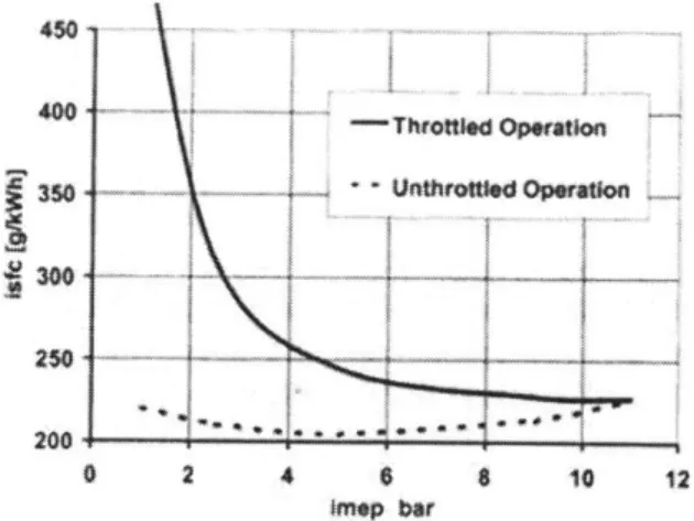
system with two catalysts; the upstream iridium catalyst was effective for the lean mixtures while the typical platinum catalyst was placed downstream. Afterwards, Toyota, Nissan, Ford, Opel, and Volkswagen among others, have developed and marketed stratified gasoline DI engines in Asia and Europe. The benefits of unthrottled operation is shown below in Figure 1-1[3].
450 400 -Throtfld Opration 31 350 Unthr.UW4Opra I... v300 200 0 2 4 6 8 10 12 Wep bar
Figure 1-1 Comparison of indicated specific fuel consumption (ISFC) between throttled and unthrottled operation as a function of engine load.
Observers of the DISI trend in these continents will wonder why the trend has not swept into the US with similar speed. One of the reasons for this delay comes from the resulting exhaust of lean operation; the optimum three-way catalyst conversion efficiency of NO,
CO, and HC hovers around stoichiometric air/fuel ratios, +/- 0.1 air/fuel ratios [4]. This
tight band of operation makes the three-way catalysts ineffective for the operating points that these Asian and European calibrations use. Consequently, the DISI engines in these markets take advantage of lean NOx catalysts, also known as selective reduction catalysts. More important than the higher cost as a barrier to entering the American market, these catalysts are poisoned by fuels with higher sulfur content, which varies significantly with different countries as shown below in Figure 1-2[5].
1000 PetmCv~ SR ular Gaso**e
800-II
... .. .. . 0 CCFigure 1-2 Worldwide sulfur concentration in gasoline (data published in 1998)
Another benefit of direct injection is the improved combustion stability as shown in reduced air/fuel ratio variation in Figure 1-3 [15].
2
0.9
0. 8
0. 9
nlaIl 1
M
Ap IMd
It
fitI fI
IF VII f
trrt
Time (se)Figure 1-3 Variation of air/fuel ratio during the 11th cycle of the LA-4 mod vehicle test
This air/fuel ratio data was obtained with an Isuzu GDI for the LA-4 mode vehicle test, and the reduced variation is readily apparent as proof of the precise fuel metering capability provided by the DISI system.
1.1.2 Efficiency
While many publications tout the fuel consumption improvements with direct injection engines, the compromises, and hence efficiency decreases from the theoretical maximum, needed to meet the emissions standards cannot be overlooked. A part load fuel
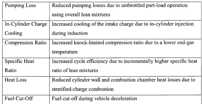
consumption reduction of 20-25% has been reported with charge stratification, depending on test conditions and optimization [2]. Zhao, et al. provided the factors contributing to this improvement in Table 1:1.
Table 1:1 Major factors contributing to the BSFC advantage of a G-DI engine as compared to that of a conventional PFI engine
Pumping Loss Reduced pumping losses due to unthrottled part-load operation using overall lean mixtures
In-Cylinder Charge Increased cooling of the intake charge due to in-cylinder injection
Cooling during induction
Compression Ratio Increased knock-limited compression ratio due to a lower end-gas temperature
Specific Heat Increased cycle efficiency due to incrementally higher specific heat
Ratio ratio of lean mixtures
Heat Loss Reduced cylinder wall and combustion chamber heat losses due to stratified-charge combustion
Fuel Cut-Off Fuel cut-off during vehicle deceleration
As mentioned previously, the charge cooling provided by the direct injection is a significant means for improving the fuel consumption of combustion engines. Since a cooler charge can increase the knock-limited compression ratio by two full ratios [6], the subsequent effect is an increased fuel conversion efficiency of 2.7% for a compression ratio increase from 10 to 12. Furthermore, Andriesse et al. estimated the fuel economy benefits with a homogeneous DISI system to be 7-10% [7]. The largest component (3-4% improvement) is
the potential for downsizing the engine while providing the same power and torque. Other improvements could be made by higher EGR capability (1.5-2%) and optimized fuel/air metering during warm-up and transient operation.
Of course, the charge cooling effect is highly dependent on several parameters, one of
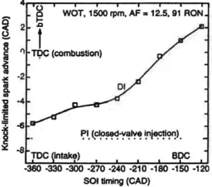
which is the start of injection (SOI) timing. In general, as the injection is advanced, the effect is magnified since the cooler charge has less time to absorb heat from the cylinder walls. As a result, the potential for efficiency improvements due to charge cooling is proportional to the SOI advance, shown in Figure 1-4[8].
j4
W6T. 150 rpM, AF 12-5. S1 RON. 2 -Tl~os mmnstconn 82Clntak,) L -360 -30 -300 -270 -240 -210 -180 -150 -120 SO timng (CAD)Figure 1-4 Comparison of knock-limited spark advance between the GDI and PFI engines
As the SOI is advanced, the charge is increasingly cooler and more resistant to knocking. Thus, the knock-limited spark can be advanced.
1.1.3
Hydrocarbon Emissions
Table 1:2 Negative factors that moderate the fuel economy potential of a stratified-charge G-DI engine Emissions Emissions constraints that may not allow the engine to operate at
the optimum brake specific fuel consumption (BSFC) point Fuel Consumption Fuel consumption penalty due to high-pressure pump and/or air
compressor for air-assisted injection
Combustion Negative impact of increased surface-to-volume ratio of a stratified-Chamber Design charge combustion system due to an increased compression ratio
coupled with a more complex piston geometry
The compromise between fuel economy benefits and reduced emissions will affect the ability to reduce throttling losses. Throttling can be reduced by lean operation of the engine, but the stability of combustion and lower exhaust temperatures limit the range of effective lean operation. Zhao et al. cited that light throttling is an effective means for controlling HC emissions while slightly decreasing fuel economy. These issues begin to illustrate the disparity between the theoretical efficiency improvement of 20-25% and the realized improvement of 10-12% [2].
1.1.4 Vaporization
One of the concerns with HC emissions is that sufficient vaporization may not occur before combustion. Vaporization can be related to the temperature of the charge, demonstrated in Figure 1-5 [8].
iOW Inte IroI
O.300
40 S 600 700 $00soAir tempratur, at IVC P(
Figure 1-5 Droplet life time under varying conditions
Saturation vapor pressure curves of normal paraffins can also illustrate the ease with which most elements will be at boiling conditions at standard cylinder wall temperatures. Despite this boiling, total vaporization is not guaranteed as discussed in the Coolant Temperature Experiment section.
Similarly to charge temperature, the fuel pressure is another factor affecting the potential for vaporization since the drop velocity and size are sensitive to this parameter, shown in Figure 1-6 [9].
25
20
15
10
5
10
15
Fuel Pressure(MPa)
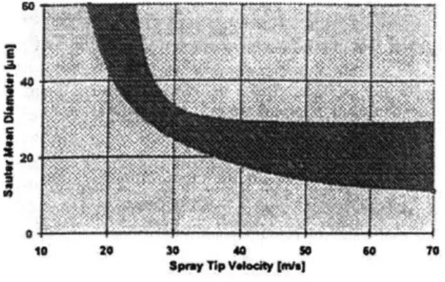
This data was taken with a Toyota swirl injector so the absolute values for Sauter Mean Diameter (SMD) and pressure may not be representative for a different design; logically, regardless of the particular injector design, the SMD will reach a lower bound despite further increases in fuel pressure. This general trend is illustrated with a large variety of injectors and fuel pressures in Figure 1-7 [11].
0 20 30 40 so 7
Figure 1-7 The effect of spray-tip velocity on Sauter Mean Diameter
Despite the common usage of SMD as a metric portraying the useful droplet size, other
values such as DV90 prove more useful in quantifying the spray's likelihood to vaporize, which heavily affects the HC emissions. The DV90 value is a function of the statistical droplet size distribution; it is the droplet diameter under which 90% of the volume is comprised with smaller droplets. The reason the DV90 can be more appropriate for
quantifying the fuel spray is illustrated in the following example: "Each 50-pm fuel droplet
in a spray size distribution having an SMD of 25-gm not only has eight times the fuel mass
of the mean droplet, but also will remain as a liquid long after the 25-prm drop has
evaporated. In fact, it is very informative to consider that when all of the 25-pm droplets are evaporated, the original 50-Rm droplets will still have a diameter of 47-pm. [2]"
Furthermore, injectors cannot be assumed to have similar distributions as illustrated below in Figure 1-8 [10]
-- of. nozzle SMDO-19.6 pM 0.05 ... - Swi nozzlesmD-16s11m, 0.043... C 0.02 S0.00 0. 2O 40 80 SO 100
Droplet diameter (pim)
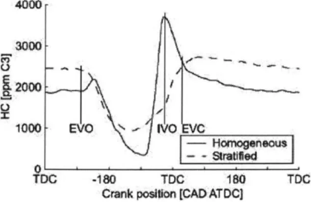
Figure 1-8 Comparison of drop size distributions for sprays from swirl-type and hole-type injectors Another research institution tested a DISI system with a wall-guided combustion system, which uses the piston to direct the fuel towards the spark plug. Of course, the stratified experiment was expected to have high HC emissions with overmixing, i.e. too lean of a mixture, at the edge of the air/fuel cloud and additional problems with undermixing in the center of the spray jet and in the case of pool burning [11]. The results obtained comparing homogeneous and stratified emissions are shown in Figure 1-9.
4000 3000-.2000 1000 EVO IVO VC --Homogeneous --Stratiled TDC -180 TDC 180 TDC
Crank position [CAD'ATDCJ
Figure 1-9 HC concentration trace for homogeneous charge and stratified charge operation with Japanese fuel (mean of 250 cycles).
The explanation for the peak in homogeneous operation is the roll-up vortex as the piston scrapes the cylinder wall and transports the unburned HC, which escaped the combustion event through the crevice and oil desorption mechanisms. Another experiment was performed to assess the role of liquid fuel in the HC trace, Figure 1-10.
4000
3000 E
EL2000
EVO ~ IVO EVC
1000
Japanese - [so-P entane
TDC -180 TDC 180 TDC
Crank position [CAD ATDC
Figure 1-10 HC concentration trace for homogeneous charge operation with 1) pre-vaporized
iso-Pentane and, 2) in-cylinder injection of Japanese fuel (mean of 250 cycles).
In this case, the significant difference after exhaust valve opening (EVO) is credited to piston impingement due to an early injection time of 30 CAD aTDC.
Another contribution to the literature included a review and comparison of the HC capabilities between the modern PFI engine and the DISI engine. Because of the poor vaporization with cold port surfaces, the standard PFI engine injects much more fuel than would be needed for a stoichiometric mixture, knowing that only a small fraction will vaporize and be transported to the cylinder. A significant amount of fuel remains on the port surfaces, creating a puddle of fuel as shown by the large amount of "port wetting fuel [12]." Note that multiport fuel injection (MPI) and port fuel injection (PFI) are used interchangeably in this text.
Engine-out HC port wetig 200 fuel 150 Burned fe Cylinder wetting 0 DISI MPI
Figure 1-11 Difference in fuel behavior between the PFI and DISI engine.
As shown in Figure 1-11 above, despite injecting quite a bit less volume of fuel, the DISI still transports more HC emissions from the engine. Furthering the comparison, the HC emissions were plotted for the DISI engine, after being normalized to a value of 100. On the other hand, the PFI emissions level was approximately 60% of that value. In order to understand the difficulty in achieving lower emissions with a DISI engine, several methods were evaluated. The first method eliminated the injection pressure transience that normally enters the process because of the fuel pump's reliance on the mechanical speed of the engine. Another method involved a late opening of the intake valve, which increases turbulence and mixing of the fuel. The third method combined the first method with the addition of late injection, which aids the vaporization of the fuel because of the warmer air charge due to its compression. The final case included three advancements: a steady state fuel pressure, late injection, and heated fuel injection. The heated fuel injection aids the vaporization even more than the other methods, although its application in production
au
0
1 2 3 4 5 6
LConventional DISI 4.2 + late injection
2.Engine Starting W/5MPa 5: 4 + heated fuel in ection
3Late intake valve opening 6: MPI
Figure 1-12 Verification of the effectiveness in reducing HC
As illustrated above in Figure 1-12, each case after the conventional DISI improves the HC emissions, but only the most complicated and expensive option can compete with the production PFI engine. As a result, manufacturers are interested in, if not skeptical of, the capability to reduce HC emissions in the DISI engine beyond the current levels achieved with the PFI engine.
Continuing the experiments above, Koga et al. reviewed the effect of early and late injection timing in a DISI engine. On a time scale, these two cases were examined, see Figure 1-13, to reveal how the HC escapes the combustion event.
400( 300( 2000 100 Exhaust streke aryInjec on Late ection 90 ISO 2 /0 30
Injection start timing ( 0 BTDC)
Figure 1-13 Engine-out HC behavior C S 0. 0. U 0
In particular, the black peak is most likely caused by the surface wetting of the fuel. Surface wetting can cause diffusion burning of the fuel; plus, a concentration of fuel at the cylinder wall is unfavorable because of the amount that will remain unburned after the flame has been quenched at the wall. Moreover, after the fuel remains unburned near the wall, the piston scrapes the wall and transports a mixture of more highly concentrated HC into the exhaust.
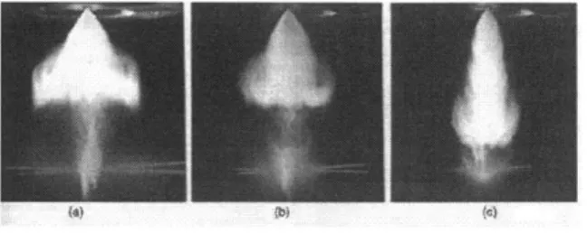
Finally, the spray pattern of fuel substantially affects the vaporization and thus, the HC emissions of a DISI [2]. While it is more common to consider the injection pressure, the ambient pressure, into which the fuel is transported, is also a parameter which can be affected by the injection timing as the intake stroke progresses or especially if the compression stroke starts, see Figure 1-14.
Figure 1-14 Effect of hot operation of a multihole injector for four levels of ambient back pressure; six-hole nozzle; 50* spray; fuel: indolene; fuel temperature: 90*C; fuel injection pressure: 11.0 Mpa; amount of fuel injected: 10 mg per injection.
As the back pressure is decreased, the individual effect of each nozzle hole becomes less pronounced, and as expected, the fuel penetration increases because the deceleration from
aerodynamic drag is smaller. Similarly, another comparison related the footprint of a spray at a location 40 mm from the injector tip, and the image was captured 4 ms after the SOI in Figure 1-15.
PAeb I b ar 9 bar 14 bar
55lb bara
Figure 1-15 Effects of back pressure (Pamb) and fuel rail pressure (Pinj) on the cross-sections of GDI sprays from a swirl injector.
As expected, the increasing injection pressure causes a greater dispersion of the droplets and a smaller droplet size. Likewise, the increasing ambient pressure causes a higher concentration of droplets given the same injection pressure. Of course, the injection
pressure increases by factors below two, but the ambient pressure is changed by an order of magnitude. Consequently, Figure 1-15 is not meant to be an exact comparison of the relative sensitivity to injection and ambient pressure. Interestingly, the injector temperature also affects the spray pattern as shown in Figure 1-16, Figure 1-17, and Figure 1-18 [2].
Figure 1-16 Effect of swirl-injector operating temperature on spray development with iso-octane at 200C, 75"C, and 100'C.
Figure 1-17 Effect of swirl injector operating temperature on spray development with indolene at 20'C, 75*C, and 100*C. Nmmt~U3~COB~ YiP ft~~PHEWs~. PA Ut,. ws~suE ~ai tim.AJELPW.M 111 P4IECY1ONP.~O IQOltP. am -20 ,44 C
DISTANCE FRM lNJECTOR AXI (mm}
20 $0
Figure 1-18 Spray SMD profiles for three injector operating temperatures.
In this case, the image was taken 1.5 ms after SOI, and the ambient pressure was 0.1 MPa. The increased temperature causes a reduced effective spray cone angle and deeper
penetration. It is notable that the temperature of the injector does not alter its operation;
14
rather, the injector temperature causes heat transfer to the fuel, until the fuel has reached an equal temperature, which alters the fuel's tendency to vaporize. More important than the pictures of penetration is the inverse relationship between temperature and the droplet
2 Experimental Setup
In order to examine the hydrocarbon emissions from a DISI engine, a test cell was designed and fabricated for a production 2005 GM Ecotec engine, which was fully instrumented. The engine has a four-cylinder inline layout, and it produces 155 hp at 5600 rpm. Important geometric details can be seen in Table 2:1.
Table 2:1 Engine geometry details
Displacement, Vd 2198 cm3
Bore, B 86.0 mm
Stroke, L 94.6 mm
Compression ratio, r, 12.0
Intake Valve Opening/Closing 00 aTDC* / 650 aBDC
Exhaust Valve Opening/Closing 10.50 bBDC* / 44.50 aTDC*
*These values are taken from an internal GM-Opel paper with clarification from Arthur Freeland [17] and have not been confirmed as factual for this particular engine. This paper lists the "duration" for the intake valve timing as 240 CAD and the "spread" as 120 CAD. The spread is defined as the CAD between TDC and the max valve lift. Hence, the intake valve opening is estimated to be at TDC. The intake valve closing time has been
experimentally verified, as it can be clearly seen in the pressure trace as the valve lands on its seat. Furthermore, the pressure traces are shown in Appendix- 1.
These valve timings can be compared to a similar PFI GM Ecotec engine in the Sloan Auto Laboratory with IVO/IVC at 7 bTDC/56 aBDC and EVO/EVC at 68 bBDC/16 aTDC.
markets [17], the exhaust valve timings are quite different from the PFI engine. The
exhaust valve opening (EVO) is supported by the pressure trace in Appendix- 1, because an earlier EVO would have produced a visible decline in pressure as the exhaust blows down from a higher pressure. Also, the EVC is supported by the results in the Injection Timing Experiment section (p. 62).
In addition, the engine utilizes Siemens injectors with a variable stock operating pressure ranging from 40 to 120 bar, and the injector is located on the side of the chamber, between the intake valves as seen in Figure 2-1. The internal GM-Opel paper does not provide information about whether the injectors are swirl injectors or simply multihole; however, it does clarify that the SMD<16pm.
Figure 2-1 iCombustion chamber; injector and spark plug location
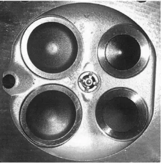
Even though the engine was produced in Europe, it was designed for homogeneous, stoichiometric operation as indicated by the lack of bowl in the piston in Figure 2-2. A
bowl shape in the piston typically denotes the potential for stratified operation by the spray-guided method of operation.
Figure 2-2 Piston shape
Since each cylinder would produce similar conclusions about the HC emissions mechanisms, all experiments have been performed on one running cylinder while the engine is motored, i.e. simply spun without fuel or combustion. As a result of this mode of operation, the intake and exhaust manifolds were separated to precisely measure and
analyze the air entering and exiting the chosen cylinder. At the same time, the flanges of the manifolds were retained for a proper seal to the engine head. The flow characteristics, e.g. velocity field, of the intake air should be representative of the stock engine since the air is divided to the two intake runners with 15 cm of the stock manifold retained.
Typical engine operation consisted of using an electric motor to determine and stabilize the engine speed, while the eddy current dynamometer, produced by Froude Consine Limited model AG30, provided a constant torque on the engine. The manifold absolute pressure (MAP) was controlled by two gate valves to inhibit the flow of the intake air.
Typical operating procedures for filling the fuel system, motoring the engine, starting the engine, and shutting down the engine can be found at the end of this chapter: Table 2:3, Table 2.:4, Table 2:5, and Table 2:6.
2.1 Instrumentation
In order to assess the engine performance and control it to a high degree, several instruments were necessary.
2.1.1 Air Flowmeter
Since the intake manifold for the firing cylinder is separated from the other three cylinders, the air flowmeter measures only the air entering the cylinder of interest. The sensor is an EPI model 8716MPNH with two-inch tube style connections on both ends; after selecting an operating range, the flowmeter has a sensitivity of 7.14 g/s / V with an accuracy of
+/-[1% Reading + (0.5% Full Scale + 0.02% / C)]. Two resistance temperature detectors (RTDs) comprise the internal sensing elements. One RTD measures the ambient
temperature, while the second RTD is heated to a higher temperature. As the flow of air increases, and hence the heat transfer from the heated RTD increases, the flowmeter measures the power needed to maintain the heated RTD's temperature. From this power consumption, the flow rate of air can be determined accurately.
2.1.2 In-Cylinder Pressure Transducer
In order to determine the engine's mean effective pressure (MEP) and other characteristics of each cycle's combustion, the engine has a Kistler 6125A pressure transducer. This
transducer was selected for the application because of its response and recommendations from industry researchers. GM performed the complicated machining into the engine head; the machining must reach a precise depth in order to minimize the volume between the combustion chamber and the tip of the transducer, without damaging the structural integrity of the combustion chamber's contour. Furthermore, this professional machining is
recommended to achieve a properly sealing sleeve between the transducer and the oil and coolant galleries. In the event that a future project requires firing additional cylinders, they have been prepared to accept the same 6125A transducer installed.
The 6125A transducer has a sensitivity of approximately -16.3 pC/bar with a linearity of +/- 0.5% of full scale. Finally, the pressure transducer is a relative measurement of pressure; as a result, the pressure signal must be "pegged" to a certain value in order to obtain meaningful results. For this application, the LabView code pegged the cylinder pressure to be equal to the MAP sensor pressure at BDC intake.
2.1.3 Lambda Meter
To acquire the air/fuel ratio information, an Etas LA4 Lambda meter is located about 17 cm from the exhaust port; it operates with a combination of a Nernst concentration cell and a pump cell to transport oxygen ions. The planar two-cell design of the lambda meter
consists of a solid body electrolyte comprised of ceramic layers, which separate a reference gas and the exhaust. The voltage produced across this planar sensor is highly sensitive to the oxygen content in the exhaust, and hence, is sensitive to the air/fuel ratio.
2.1.4 Fast Flame Ionization Detector
The primary tool for exhaust analysis was a Cambustion HFR-400 Fast Flame Ionization Detector (FFID) with a time response (10-90%) of approximately one millisecond [18]. The instrument was calibrated before and after each experiment using 1500 ppm C3 (4500 ppm C1) propane (C3H8) span gas and zeroed with ambient air. Time-averaged
downstream HC emissions were sampled from a well-mixed, large volume, pulse-dampening tank located 180 cm from the exhaust port.
2.2 Systems
Due to the operation of internal combustion engines, several parts of the experimental setup are best explained through a system view.
2.2.1 Intake System
The intake air enters the system through a filter and flows through the aforementioned air flowmeter. Next, a parallel arrangement of gate valves allows fine and broad control of the flow; this arrangement replaces the function of a throttle, which would be harder to control and unnecessarily complicate the system since the manifold absolute pressure (MAP) was seldom varied. Downstream of the valves, a tank is used to dampen the pressure
oscillations created by the periodic vacuum of the cylinder. The volume of the tank is approximately ten liters, chosen specifically to be a factor of 20 increase of the displaced volume of the active cylinder. The hose connecting the damping tank to the intake
manifold is rated to a full vacuum, i.e. 29.9 mm Hg, and it has a smooth inner contour. The hose is attached to the intake manifold through a wire clamp and further sealed with silicon
tape. Despite the large number of pipe and hose fittings, the quality of the intake system, and its lack of leaks, is shown by the 0.07 bar vacuum that the system can sustain with the gate valves completely closed. Thus, the intake airflow rate can be accurately determined
by the air flowmeter.
2.2.2 Fuel System
The stock engine employs a mechanical fuel pump driven by the camshaft, but for the purposes of controlling the injection pressure independently of speed, this setup utilizes the system shown in Figure 2-3.
Pressur e R egulator Hy draulic Accumulator Tank Che ck Valve Fuel Filter
Fuel Rail and Injectors
Pressure
Gauge Fuel
Pump
Fuel Tank
The primary component of the fuel system is the hydraulic accumulator, which is a high-pressure vessel with an internal piston. One side of the piston is pressurized with nitrogen from a tank, which has a fully charged pressure of 160 bar. The pressure in the line and in the accumulator is controlled by the manual pressure regulator. The other side of the accumulator piston can be filled with fuel by the electrical pump. It is important to note the significance of the check valve in the system to ensure the highly pressurized fuel does not travel back to the fuel tank. The second connection on the pressurized side of the
accumulator is a line supplying fuel to the common rail and operating injector. The fuel system is limited to 135 bar (2000 psi) by the strength of the stainless steel tubing used for the high-pressure lines. The fuel injectors were calibrated with a custom rig to capture the spray in a vial which sealed to the circumference of the injector. The calibration is shown in Appendix- 2.
2.2.3 Coolant System
For the purpose of investigating the vaporization achieved in this DISI engine, the coolant system was designed to reach a wide range of coolant temperatures. The two ball valves allow two coolant loops: one to heat and one to cool. The details and operation of the coolant system is shown in Figure 2-4.
City W Solenoid Valve
(normally open)
Heat Exchanger
Engine Block
1
Tee Ball ValveSt
ater
F Tee Ball Valve
IF
Coolant
Tank
Coolant Pump
Figure 2-4 Coolant system diagram
First, the heating loop is achieved with both handles of the valves aligned with the singular port of the pipe tee. For chiller usage, both handles should be parallel with the two ports of the pipe tee. The 10 KW heater provides a relatively quick ramp up in the coolant
temperature, and 80*C was generally used as the maximum temperature. A simple controller was used to regulate the coolant temperature within a certain range. If the coolant temperature, measured entering the engine, dips below the lower set temperature, then the controller sends a signal to close the solenoid valve of the cooling water and to turn on the heater. Likewise, if the temperature increases beyond the high set point, the controller opens the solenoid valve to the heat exchanger water and simultaneously turns
off the heater. The lower bound of the coolant temperature for steady state operation is
about 20'C, depending on the ambient temperatures.
2.2.4 Exhaust System
In a similar manner to the intake manifold, the exhaust manifold was separated so that measurement samples were only taken from the running cylinder. The lambda sensor and first thermocouple are located approximately 18 cm from the exhaust port. Since the first set of experiments were planned to examine steady state operation, a mixing tank, located about 180 cm from the exhaust port, was placed in the exhaust line so that the exhaust species would be spatially homogeneous. After mixing, the exhaust temperature and FFID ports were located in the exhaust stream.
2.2.5 Engine Control System
The engine control system consists of a master and slave computer. The master computer accepts the user inputs of engine speed (RPM), target lambda value, end of injection (EOI, in CAD aBDC compression), and spark timing (CAD aBDC compression). Its C program calculates the start of injection (SOI) and the dwell in crank angle degrees. The dwell is the amount of time that the spark plug needs to be charged before it emits its spark. The master program places this information into an array which is sent to the slave computer.
The slave computer must run its C program in DOS since the computations for small actions, like moving the mouse, have the potential to cause the outputs enough delay that the engine could misfire for a cycle. The slave program accepts the inputs of feedback gain
operation of the injector and the spark plug. A hardware switch is used to interrupt the engine's operation and ensure that the sequence of injecting and firing is stopped with the injector in the closed position.
2.2.6 Data Acquisition System
The data acquisition system is based upon a National Instruments platform, schematically shown in Figure 2-5; a description of its components and the respective purposes is given in Table 2:2.
Chassis -SCXI 100X
Tle oeouph Data
SCXI 1112 1
Master Campuder Tower
BNC 2095
S 1349P622
BDC aampress
sitinl syte Crank Augle signal
Table 2:2 Data acquisition components and functions
Item Function
BNC 2095 Records up to 16 differential analog BNC signals
SCXI 1112 Records up to 8 thermocouple signals
SCXI 1100 Multiplexes the signals into a single programmable gain instrumentation amplifier (PGIA)
SCXI 1302 Allows digital signals to feed through to the master computer
SCXI 1349 Necessary adapter to include the feed through signals
PCI 6220 Data acquisition card
The data was acquired through a LabView program, and the majority of data was recorded on a crank angle basis, except temperature data, which cannot be recorded as quickly.
Table 2:3 Fuel filling procedure
1. Depressurize the nitrogen line by turning the pressure regulator several
counter-clockwise turns until there is only ambient pressure in the line and accumulator.
2. Ensure that sufficient fuel exists in the ATL tank by lifting the tank to gauge its weight (if the fuel pump is activated without enough fuel in the tank, the line will be filled with air and will need to be purged).
3. Remove the blue cap to allow air flow into the tank.
4. Turn on the fuel pump at the control panel. The pressure gauge on the system should read about 25 psi while filling the accumulator, and it will rise to the relief valve
threshold (80 psi) when the accumulator is full. Filling a completely empty accumulator should take approximately 75 seconds from the measured flow rate.
5. Turn off the fuel pump.
6. Replace the blue cap on the ATL tank; if the fuel is left open to atmosphere the
vaporization is not only a danger, but it lowers the remaining fuel's volatility.
7. Allow flow from the nitrogen bottle by turning the knob counter clockwise. 8. Pressurize the nitrogen line by turning the pressure regulator knob clockwise.
Table 2:4 Engine motoring procedure 1. Turn on the lab fan and water pump.
2. Allow flow from the nitrogen bottle by turning the knob counter clockwise.
3. Pressurize the nitrogen line by turning the pressure regulator knob clockwise.
4. Ensure the National Instruments chassis is powered.
5. Flip the motor breaker to the "on" position, normally allowed 5 minutes to warm up.
6. Check the rotating parts for possible obstructions or wires in their path.
7. Check oil level with the dipstick and coolant level through the sight tube on the tank. 8. Check that the coolant valves on the test bed are in the proper position.
9. On the wall, adjust the ball valves directing water flow to the dynamometer, coolant
heat exchanger, and oil heat exchanger. Unless specifically needed, the valves should be opened with a maximum of 300. If the valves are open too far, the water pressure will be
insufficient for other test cells. Small flow rates for the coolant heat exchanger can help the stability of the engine coolant temperature.
10. Open main water valve to allow water flow.
11. Turn on the sensor switch, labeled Lambda and Mdot, at the control panel. Enter the
test cell to press the "operate" button on the pressure transducer amplifier.
12. Turn on the dyno controller by the right button. (Do not press the left button, which engages the dyno. It will be engaged after starting and motoring the engine).
13. Turn on the coolant pump switch, at the control panel.
14. If experiments are highly temperature dependent, turn on the oil pump and chiller toggle switches. To engage the oil pump, push the start button on the oil pump controller located on the tower in the test cell. Note the heater controller should stay in stand-by "Stby" mode until the engine is started, to avoid the potential to vaporize the coolant with the high powered heater.
15. Turn on the motor controller switch at the control panel. Shortly thereafter, the motor controller will make a higher pitched sound as it enters the overdrive mode.
16. After hearing this sound, briefly crank the engine with the key on the control panel.
The duration should be no longer than 1-2 seconds. If the crank time is appropriate, the motor will spin the engine as shown by the rotation of the crankshaft, which can be seen from the test cell window. If the crank time is too short, try a slightly longer duration.
17. The motor controller value corresponds to the engine speed, which can be read on the
dyno controller. For example, a value of 25.2 corresponds to 1230 rpm, which is then reduced to 1200 rpm as the dyno is engaged.
Table 2:5 Engine running procedure
1. After following the Engine Motoring Procedure, turn the dyno load set point (LSP) to
zero. Now press the left button on the dyno controller; the engine will slow down for a few seconds, but the motor will ramp the speed back up to its initial value.
2. Slowly increase the load to the desired set point, which will slow down the motor, for example from 1230 rpm to 1200 rpm.
3. Both the slave and master computers should already be on. The slave computer should
be running in DOS mode, not simply a DOS command prompt; the operating file is located in C:\D\singleb. The master computer should use a command prompt to access its program located in C:\D\master b.
4. On the master computer, enter the rpm as read from the dynamometer controller.
5. When prompted, enter the target lambda value, the injection timing (e.g. 660 CAD aBDC), and the spark timing (e.g. 160 CAD aBDC).
6. When prompted, enter the feedback gain (e.g. 10) and the injection duration (e.g. 1700
psec), and press enter.
6. After hitting enter, the engine sound will change assuming good combustion is
achieved as shown by the lambda meter readout.
7. If the lambda readout is extremely rich (below 0.7) or extremely lean (1.3), stop the
engine running program with the hardware switch located in the desk. Problems starting combustion can be diagnosed by logging data after completing step 6, see step 10.
8. After motoring the engine for a minute, reattempt to get the engine running, ie step 4.
The motoring process alleviates the chances of backfiring the excess unburned fuel from the previous step.
9. Follow the Omega controller instructions to us the coolant temperature controller.
Essentially, the controller will attempt to keep the coolant inlet temperature between two set values. If the coolant becomes too warm, the controller will send a signal to open the solenoid to run water through the heat exchanger. If the coolant becomes too cool, the heater will turn on the heater located in the coolant tank.
Table 2:6 Engine shut-down procedure
1. Press Enter twice on the coolant temperature controller to put it into stand-by mode.
2. Flip the hardware switch to end the engine running program, which ends the program running on the slave computer. The sound of the engine should change frequency. The master computer can be exited with three zeros (0 0 0).
3. Turn the appropriate instruments (including coolant pump) off at the control panel.
4. Disengage the dyno by deactivating the left button.
5. Turn off the motor with the switch on the control panel, and the engine should reach zero rpm within a few seconds.
6. Turn off the dyno controller power with the right button. 7. Flip off the motor breaker inside the test cell.
8. The National Instruments chassis and control panel power supply can be left on. 9. Stop the flow of water by closing the main water supply valve. The other valves can
be left in their position for convenience for the next experiment.
10. Ensure the blue fuel cap is finger-tight on the ATL tank. 11. Close the nitrogen tank by turning its knob clockwise.
12. Drain the nitrogen in the system, unless experiments will be run within one day. The extra pressure in the system is not ideal if something were to break or the fuel system leaks a few drops of fuel due to the high pressure, but draining and filling the lines every time hurts the usage time of each nitrogen tank.
3 Results
In order to achieve a common basis for comparison of the experiments, a baseline condition was determined. These conditions are listed in Table 3:1.
Table 3:1 Baseline operating conditions
The engine speed and manifold absolute pressure (MAP) were selected to represent the fast idle period. The injection timing is always listed as the end of the injection (EOI). For comparison to papers listing SOI, the start of injection timing can be approximated from the pulse width of 15 CAD. While 15 CAD is easy to visualize on the graphs of data, when a more accurate value is needed, a more precise pulse width of 12.7 CAD was calculated from the mass flow rate of air, the lambda value, and the injector calibration. The fuel pressure baseline was selected as a pressure in the middle of the stock engine operation, which is variable from 40-120 bar. Finally, the coolant temperature was selected to be quite warm at 60'C, but 800C was not chosen because of the additional time that every
experiment would take to warm up to steady state.
As a result of the control systems installed, some of the baseline parameters had a slight variation. For example, the MAP experienced some fluctuation, but it was maintained
Engine Speed 1200 rpm
MAP 0.46 bar
End of Injection Timing 120 CAD aTDC
Fuel Pressure 70 bar
Coolant Inlet Temperature 600C
universally within +/- 0.015 bar. Similarly, the manual control of the nitrogen pressure regulator caused a difficulty in matching the exact desired fuel pressure. Across all experiments, the fuel rail pressure was kept within a +/- 1.5 bar tolerance. The coolant temperature was controlled within +0.51-1.0 C of the target value. In general, the experiments were repeated on two separate days, and each point within the experiments was logged two to four times with about 50 cycles worth of data recorded each time. Hence, the plots generally represent at least 200 cycles of averaged HC data. The exceptions to this rule are the Injection Pressure Experiment with High DI fuel and all isopentane tests, which include 100 cycles of averaged HC data.
Given the capability of the experimental setup, five sets of experiments were performed to illustrate the underlying mechanisms of HC emissions as shown in Table 3:2. Each of these experiments was completed during steady state operation.
Table 3:2 Engine parameter experiments
1. Sweep of coolant temperatures at baseline conditions
2. Sweep of injection pressure at baseline conditions
3. Sweep of injection timing at baseline conditions
4. Sweep of injection timing at varying coolant temperatures 5. SwNeep of injection timing at varying injection pressures
The above experiments were also repeated with two types of fuel, Chevron Phillips UTG91 and a High DI fuel, with the properties of the former given in Table 3:3.
Table 3:3 Chevron Phillips UTG 91 fuel
Property
Specific Gravity at 60/60 OF API Gravity
Copper Corrosion, 3 h at 50 *C
Existent Gum (washed), mg/100 mL
Suifur, ppm
Reid Vapor Pressure, psia
Lead, gfgal
Phosphorus, gigal
Hydrogen, wt %
Carbon, wt %
Carbun Density, gigal
Distillation Range at 760 mming, 'F
Initial Boling Point
10% 50% 90%
End Point Oxidation Stablity, min Ileat of Conustion, Net, Btlb Composition, vol %
Aromatics
Olefn
Saturates Research Octane Number Motor Octane Number
Anti-Knock Index, (R+M)2
Sensitivity Oxygenates, vol % Benrene, vol %
The second fuel had the following specifications written on the barrel: 1250 DI QF 1721
LS 04 Haltermann Gasoline 3 UN1203 II ERG 128.
The driveability index (DI) is calculated by the following formula:
DI= 1.5 * T10 + 3 *T50 + T90
DI= 1.5 * 122 + 3 * 212 + 321 =1140
(1)
(2) (for the UTG 91 example)
Where T10, T50, and T90 are the distillation temperatures (OF) at the 10%, 50%, and 90% distillation points; hence, UTG 91 has a DI of 1 1400F. On the other hand, the second fuel
has a DI of 12500F; this fuel will be referred to as "High-DI" fuel. Granted, not all effects
on HC can be so easily linked with the lower volatility of the second fuel because of the complications of boiling heat transfer, but they are expected to be closely related.
Typical Value 0.7350 61.0 1 2 130 9.0 0.0010 0.001 13.7 86.3 88 122 212 321 399 >1440 18500 24.0 6.0 70.0 90.8 828 86.8 7.8 Specification 0.7343 -0.7440 Report I max 5 max 1000 max 8.8-9.2 0.0050 max 0.0D2 max Report Report Report 75-95 120- 135 200- 230 300- 325 415 max 1440 min Report 35.0 max 10.0 max Report 90.3-917 Report 87.0 max 7.5 min 0.0 max Report Test Method ASTM D 4052 ASTM D 1250 ASTM D 130 ASTM D 381 ASTM D 5453 ASTM D 5191 ICP/OES ICPIOES ASTM D 5291 ASTM 0 5291 Calculated ASTM D 86 ASTM D 525 ASTMI D 240 ASTM D 1319 ASTM 0 2699 ASTM D 2700 Calculated Calculated Chromatography Chromatography