An analysis of the effect of Gaussian error in object recognition

(1)

An Analysis of the Effect of Gaussian Error in

Object Recognition

by

Karen Beth Sarachik

B.A., Barnard College (1983)

S.M., Massachusetts Institute of Technology (1989)

Submitted to the Department of Electrical Engineering and

Computer Science

in partial fulfillment of the requirements for the degree of

Doctor of Philosophy

at the

MASSACHUSETTS INSTITUTE OF TECHNOLOGY

February 1994

o

Massachusetts Institute of Technology 1994

7/? .

Signature of Author ...

. ..

-.-.

.. ..., ...

Department of Electrical Engineering and Computer Science

January 7, 1994

Certified by ...

.. . ..

-.

. . ..A

-..-.

...

W. Eric L. Grimson

Associate Professor of Computer Science and Electrical Engineering

,-

•.

Thesis Supervisor

A ccepted by ...

_.Fre _R.V _.M...

F

Zr

-R. Morgenthaler

on Graduate Students

--Chairman.

(2)

(3)

An Analysis of the Effect of Gaussian Error in Object

Recognition

)by

Karen Beth Sarachik

Submitted to the Department of Electrical Engineering and (Computer Science on January 7, 1994, in partial fulfillment of the

requirements for the degree of Doctor of Philosophy

Abstract

In model based recognition the problem is to locate an instance of one or several known objects in an image. The problem is compounded in real images by the presence of clutter (features not arising from the model), occlusion (absence in the image of features belonging to the model), and sensor error (displacement of features from their actual location). Since the locations of image features are used to hypothesize the object's pose in the image, these errors can lead to "false negatives", failures to recognize the presence of an object in the image, and "false positives", in which the algorithm incorrectly identifies an occurrence of the object when in fact there is none. This may happen if a set of features not arising from the object are located such that together they "look like" the object being sought. The probability of either of these events occurring is affected by parameters within the recognition algorithm, which are almost always chosen in an ad-hoc fashion. The implications of the parameter values for the algorithm's likelihood of producing false negatives and positives are usually not understood explicitly.

To address the problem, we have explicitly modelled the noise and clutter that occurs in the image. In a typical recognition algorithm, hypotheses about the position of the object are tested against the evidence in the image, and an overall score is assigned to each hypothesis. We use a statistical model to determine what score a correct or incorrect hypothesis is likely to have. We then use standard binary hypothesis testing techniques to decide the difference between correct and incorrect hypotheses. Using this approach we can compare algorithms and noise models, and automatically choose values for internal system thresholds to minimize the probability of making a mistake. Our analysis applies equally well to both the alignment method and geometric hashing.

Thesis Supervisor: W. Eric L. Grimson

(4)

(5)

Acknowledgments

I have spent many years at the MIT AI Lab, and have many people to thank for my association with them during that time.

Eric Grimson has been a patient and supportive advisor, and helped me start out on the original problem. This thesis was improved tremendously by the meticulous

reading and careful comments of Professor Jeff Shapiro.

I have benefited greatly from technical discussions with Sandy Wells, Randy Godwin, Marina Meila, David Clemens, David Jacobs, and Mike Bolotski, as well as from their friendship.

My friendship with many other lab members was a constant source of support, in-cluding David Siegel, Nancy Pollard, Ray Hirschfeld, Marty Hiller, Ian Horswill, Paul Viola, Tina Kapur, Patrick Sobolvarro, Lisa Dron, Ruth Schoenfeld, Anita Flynn, Sundar Narasimhan, Steve White, and in particular, Jonathan Amsterdam, Nomi Harris, and Barb Moore. I would also like to thank Mary Kocol, Michele Popper and Rooth Morgenstein for being extra-lab friends.

Lastly, I would like to thank my family, and Joel.

This report describes research done at the Artificial Intelligence Laboratory of the Massachusetts Institute of Technology. This work has been supported in part by NSF contract IRI-8900267. Support for the laboratory's artificial intelligence research is provided in part by the Advanced Research Projects Agency of the Department of Defense under Office of Naval Research contract N00014-91-J-4038.

(6)

(7)

List of Figures

1-1 Stages in model based recognition. . ... . . . ... 2 1-2 Recovering information from a source over a noisy channel. ... 4 2-1 Possible positions of a model point due to positional uncertainty in the

three points used in the correspondence to form the pose hypothesis. 15 3-1 Calculating the affine coordinates of a fourth model point with respect

to three model points as basis ... 20 3-2 The top and bottom figures show the location and density of the

pro-jected uniform and Gaussian weight disks, respectively. The darkness of the disk indicates the weight accorded a point which falls at that location. The three points used for the matching are the bottom tip of the fork and the ends of the two outer prongs. The image points found within the weight disks are indicated as small white dots. Note that the uniform disks are bigger and more diffuse than the Gaussian disks. 26 3-3 The density functions fpelH(P) and felH(p), respectively . ... 31 3-4 The figure shows the boundaries for the integration for both fv,(v)

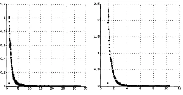
and fvy(v Im = 1). The bottom curve is a - , and the upper curve is a = _{The third dimension of the graph (not illustrated)} are the joint density functions fVM,4e(V, a) and fv_,ae,(v, I m = 1). 34 3-5 Distributions fv,(v) and fv,(v 7m = 1) for v > 0. For these

distri-butions, Co = 2.5. Note that the scale of the y axis in the first graph is approximately ten times greater than that of the second. ... . 37

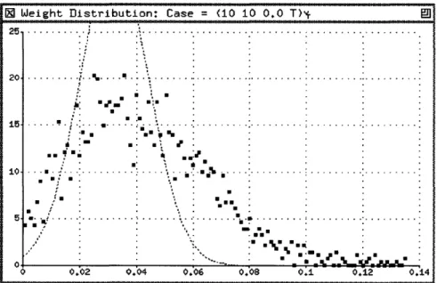
3-6 Comparison of predicted to empirical density of WH, for m = 10,

n = 10, c = 0, and a0 = 2.5. Note that the empirical density has much greater variance than predicted. . . . ... . . . 43

(11)

4-1 On the left is displayed the conditional probability density functions

fx (x Ho) - N(1,.25) and fx(x

I

Hi) - N(3, 1) of a random

vari-able X. On the right is the associated ROC curve, where PF and Por correspond to the x and y axes, respectively. On the left graph, the boundaries xl = -0.76 and x2 = 1.42 implied by the value y- = -1.76 are indicated by boxes. On the right, the ROC point for this 7 value is shown. The PF and PD values are obtained by integrating the area under the curves fx(x I Ho) and fx(x

I

H1) respectively, outside the boundaries. The integration yields the ROC point (0.2, 0.94)... 47 4-2 Comparison of predicted to empirical curves for probability of false

alarm, probability of detection, ROC curves. The empirical curves are indicated by boxes. The axes for graphs, from left to right, are (x, y) =

(0, PF), (0, PD), and (PF, PD). For all graphs, m = 10, 0o = 2.5. From

top to bottom, n = 10, 100, 500, 500, occlusion = 0, 0, 0, 0.25. ... 50 5-1 _{Comparisons of uniform and Gaussian weight disks for m}₌_{10, n}₌_10,

50, 100, 500, 1000. Left: uniform weight disk, right: Gaussian weight disk. Top: Occlusion=0, bottom: occlusion=0.25. For all ROC curves, the x and y axes are PF and PD, respectively. A low threshold results in an ROC point on the upper right corner. As the threshold increases, the performance (PF, PD) moves along the curve toward the lower left corner. . . . .. . 55 5-2 The graphs show the comparison of ROC curves for Scheme 1 (top

curve) versus Scheme 3 (bottom curve). The x and y axes are PF and PD, respectively. Increasing (PF, PD) corresponds to a decreasing threshold for the direction of The (m,n) pairs are (10,100), (10,500),

(30,100), and (30,500). For all graphs, occlusion = 0 and ao = 2.5. . . 61 5-3 Comparison of predicted to empirical curves for probability of false

alarm, probability of detection, and ROC curves for Scheme 3. The empirical points are indicated by boxes. The axes for graphs, from left to right, are (x, y) = (0, PF), (0, PD), and (PF, PD). For all graphs,

m = 10, occlusion = 0, cr0 = 2.5. From top to bottom, it = 10, 100, 500. 62 5-4 Comparison of empirical ROC curves for Schemes 1 and 3. In all graphs

the ROC curve for Scheme 1 is above that of Scheme 3. The axes are

(x, y) = (PF, Pr). For all graphs, m = 10, occlusion = 0, uo = 2.5.

(12)

6-1 First image group. The group consists of 5 images of a telephone, same lighting conditions and smoothing mask. The top figure shows one of the images of the group, with the intersection of straight line segment features from all 5 images of the group superimposed in white. The bottom figure shows the result after (Canny edge detection and chain-ing. The straight line segments from which the intersection points were taken is not illustrated. Superimposed on the bottom figure are the location of the clusters chosen for the noise measurements, indicated by circles. All intersection features located within the bounds of the circle were used as sample points for the noise measurement. ... 68 6-2 Left hand side, from top to bottom: the histograms of the x, y and z

coordinates of the intersection features depicted in the previous figure. For intersection features, the z coordinate is the angle of intersection. The Glaussian distribution with mean and variance defined by the his-togram is shown superimposed on the graph. On the right hand side is the cumulative histogram, again with the cumulative distribution superim posed . . . . 69 6-3 Second image group, consisting of the edges from 5 different smoothing

masks of the same image. Again, the top figure shows one of the images of the group, but the features shown are the center of mass features from the boundary, randomly broken into segments of length 10. The bottom figure show the clusters, i.e., groups of features which mutually agree upon their nearest neighbor features across all of the images. . . 70 6-4 Histograms of the x, y and z coordinates of the center of mass features

depicted in the previous figure. For this feature type, the z coordinate is the angle of the tangent to the curve at the center of mass... . 71 6-5 Third image group - an army knife under 5 different illuminations.

The top figure shows one of the images of the group, with the maximum curvature features from all 5 images superimposed. . ... 72 6-6 Histograms of the x, y and z coordinates of the maximum curvature

features depicted in the previous figure. The z coordinate is the

mag-nitude of the curvature ... 73

6-7 The top figure shows the original image, with the feature points chosen for the model indicated in white. The middle figure is a correct hy-pothesis that exceeded the predicted threshold, and the bottom shows an incorrect one. The points indicate image feature points, and the circles indicate projected weight disks. . ... 80 6-8 The histogram for the weights of incorrect hypotheses chosen from the

original image. Note that the mean and variance greatly exceeds those of the predicted density of W7 for rn = 30, n = 248. . ... 81

(13)

6-9 The histogram of W- for 2500 randomly chosen hypotheses For this model and image, m = 30, n = 248, when the clutter is uniform and the model does not appear in the image. The prediction closely matches the em pirical curve ... .. ... .. .. .. .. ... .. .. .. .. .. 81 6-10 The top picture shows the model present in the image, but with the

clutter points redistributed uniformly over the image. The actual den-sity of W- closely matches the predicted denden-sity. . ... . . 82 6-11 When the model points are displaced to the top of the image, the

resulting density of WH is affected, but in the other direction. That is, the noise effects are now slightly overestimated instead of underestimated. 83 6-12 The incorrect hypotheses that fell above the threshold chosen to

main-tain a PF of 0.01. For these experiments, •o = 2.0. The circles show the locations of the projected weight disks, while the points show the

feature locations. ... 87

6-13 The top figure shows the original image, with the feature points chosen for the model indicated in white. The middle figure is a correct hy-pothesis that exceeded the predicted threshold, and the bottom shows

an incorrect one. ... 89

6-14 The model of the fork superimposed in white onto the original image. 90 6-15 Three kinds of false positives that occurred for a highly symmetric model. 91

(14)

List of Tables

3.1 A table of predicted versus empirical means and variances of the dis-tribution fwH(w), in the top table, and fwH-(w) in the bottom table, for different values of m and n. ... ... . 42 6.1 Results of experiments for the telephone. The first column is the ao

value that was assumed for the experiment. The second and third columns contain the user specified PF or PD. In the fourth column is the total number of hypotheses tested. The fifth, sixth and seventh columns contain the expected number of hypotheses of those tested that should pass the threshold, the actual number of hypotheses that pass the threshold, and the error bar for the experiment (we show one standard deviation = tPF(1 - PF), t = number of trials). The actual

PF (or PrD) is shown in the eighth column. The last column shows the average distance of all the hypotheses that passed the threshold from

E[W H]... . . .. . . .. . . .. . .. . . .. .. . .. . . . ... 86

6.2 Experimental results for the army knife. Though ao for this image group was determined to be 1.8, we see that the predictions for a value of •o = 2 or 3 are much better. The columns indicate the 0-o used

for the experiment, either PF or PD , the total number of hypotheses tested, the expected number of hypotheses to score above the threshold, the actual number that scored above the threshold, and the error bar for this value (we show one standard deviation = tPF(1 - PF), t =

number of trials). The actual PF (or Pr) is shown in the next column, and the last column shows the average distance of all the hypotheses that passed the threshold from E[WH] .... 88 6.3 Experimental results for the fork model. . ... 92

(15)

6.4 Experimental results when all the points in the image bases tested come from the model. The first and second columns contain the model and

co tested. The next columns contain the specified PF , total number of

hypotheses tested, and number of hypotheses that passed the thresh-old. The next two columns contain the actual PF for this experiment and the value for the same experiment in which the tested image bases are not constrained to come from the model (this value was taken from the previous group of experiments. Finally the last column is the error bar for the experiment, which we took to be one standard deviation

= tP (1 - P ), t= number of trials. ... . 93 6.5 Experimental results when uniform clutter is assumed. The first and

second columns contain the model and •0 tested. The next columns contain the specified PF , total number of hypotheses tested, and num-ber of hypotheses that passed the threshold. The next two columns contain the actual PF for this experiment and the value for the same experiment in which the effective density is calculated per hypothesis, and the threshold dynamically reset. . ... . 93

(16)

(17)

Chapter 1 Introduction

1.1 Motivation

In order to build machines capable of interacting intelligently in the real world, they must be capable of perceiving and interpreting their environs. To do this, they must be equipped with powerful sensing tools such as humans have, one of which is Vision - the ability to interpret light reflected from the scene to the eye. Computer Vision is the field which addresses the question of interpreting the light reflected from the scene as recorded by a camera. Humans are far more proficient at this visual interpretation task than any computer vision system yet built. Lest the reader think that this is because the human eye may somehow perceive more information from the scene than a camera can, we note that a human can also interpret camera images that a computer cannot - that is, a human outperforms the computer at visual interpretation tasks even when limited to the same visual input.

Model based recognition is a branch of computer vision whose goal is to detect the presence and position in the scene of one or more objects that the computer knows about beforehand. This capability is necessary for many tasks, though not all. For example, if the task is to navigate from one place to another, then the goal of the visual interpretation is to yield the positions of obstacles, regardless of their identity. If the task is to follow something, then the goal of the interpretation is to detect motion. However, if the task is to count trucks that pass through an intersection at a particular time of day, then the goal of the task is to recognize trucks as opposed to any other vehicle.

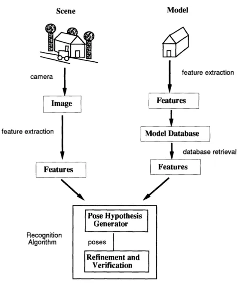
Model based recognition is generally broken down into the following conceptual mod-ules (Figure 1-1). There is a database of models, and each known model is represented in the database by a set of features. In order to recognize any of the objects in a scene, an image of the scene is taken by a camera, some sort of feature extraction is done on the image, and then the features from the image are fed into a recognition algorithm along with model features retrieved from the model database. The ta.sk of the recognition algorithm is to determine the location of the object in the image,

(18)

Scene

Model

xtraction camera Image feature extraction I database retrieval SFeatures Features Recognition Algorithm

Figure 1-1: Stages in model based recognition.

thereby solving for the object's pose (position of the object in the environment). A typical recognition algorithm contains a stage which searches through pose hy-potheses based on small sets of feature correspondences between the model and the image. For every one, the model is projected into the image under this pose assump-tion. Evidence from the image is collected in favor of this pose hypothesis, resulting in an overall goodness score. If the score passes some threshold 0, then it is accepted. In some algorithms this pose, which based on a small initial correspondence, may be passed onto a refinement and verification stage. For the pose hypothesis generator, we use the term "correct hypothesis" to denote a pose based on a correct correspondence between model and image features.

If we knew in advance that testing a correct hypothesis for a particular model would result in an overall score of S, then recognizing the model in the image would be particularly simple - we would know that we had found a correct hypothesis when we found one that had a score of S. However, in real images there may be clutter,

Pose Hypothesis Generator poses Refinement and Verification

C

17T

(19)

occlusion, and sensor noise, each of which will affect the scores of correct and incor-rect hypotheses. Clutter is the term for features not arising from the model; such features may be aligned in such a way as to contribute to a score for an incorrect pose hypothesis. Occlusion is the absence in the image of features belonging to the model. This serves to possibly lower the score of a correct hypothesis. Lastly, sensor noise is the displacement of observed image features from their true location.

If we knew that part of the model was occluded in the scene and yet we keep the threshold for acceptance at S, we risk the possibility of the algorithm's not identifying a correct hypothesis, which may not score that high. Therefore, we may choose to lower the threshold for acceptance to something slightly less than S. However, the lower we set the threshold, the higher the possibility that an incorrect hypothesis will pass it. The goal is to use a threshold which maximizes the probability that the algorithm will identify a correct hypothesis (called a true detection) while minimizing the probability that it accepts an incorrect one (called a false alarm).

In this thesis, we determine the implications of using any particular threshold on the probability of true detection and false alarm for a particular recognition algorithm. The method applies to pose hypotheses based on minimal correspondences between model and image points (i.e., size 3 correspondences). We explicitly model the kinds of noise that occurs in real images, and analytically derive probability density func-tions on the scores of correct and correct hypotheses. These distribufunc-tions are then iused to construct receiver operating characteristic curves (a standard tool borrowed from binary hypothesis testing theory) which indicate all possible triples of

(thresh-old, probability of false positive, probability of true positive) pairs for an appropriately

specified statistical ensemble. We have demonstrated that the method works well in the domain of both simulated and actual images.

.1.2

Object Recognition as Information Recovery

To approach the problem in another way, we can think of the object recognition problem as a process of recovering a set of original parameters about a source. In this abstraction, there is some sort of information exchange between the source and the observer, the information might be corrupted in some fashion, the observer receives sonme subset of the information with added noise, and finally, processes the observed iniformation in one or several stages to settle upon a hypothesis about the parameters of interest.

For example, in the case of message transmission, the parameters of interest are thie message itself, the noise is introduced by the channel, and the observer tries to recover the original transmitted message. In sonar based distance measurement, the parameter of interest is the free distance along a particular direction from a source, thIe infornmation is the reflected sonar beam, and the perceived information is the time delay between sending and receiving the beam. The observer then processes this information to derive a hypothesis about the free space along the particular direction.

(20)

Source C>+)- Observer - xform --- xform - ANSWER

z

Figure 1-2: Recovering information from a source over a noisy channel.

In model based vision, the parameters of interest are the presence or absence of a model in a scene, and its pose in three dimensional space. The information is the light which is reflected from a source by the objects in the scene, and the perceived information is the light which enters the lens of a camera. The information goes through several processing stages to get transformed into a two dimensional array of brightness values representing an image, and then through several more steps to come to a hypothesis about the presence and pose of any particular model.

In this thesis we cast the problem as a binary hypothesis testing problem. Let the hypothesis H be "model is at pose P". We are trying to reliably distinguish between

H and H. It is generally not always possible to do this, especially as the noise goes

up, but we can bound the probability of error as a function of the statistics of the problem, and can determine when the noise is too high to distinguish between the

two hypotheses.

1.3 Overview of the Thesis

All of the definitions, terminology, conventions and formulas that we will use in the thesis are given in Appendix A.

Chapter 2 explains the model based recognition problem in more detail, and gives a very general overview of work relevant to this thesis. We will define the terms and concepts to which we will be referring in the rest of the work.

In Chapter 3 we present the detailed error analysis of the problem.

In Chapter 4 we present the ROC (receiver operating characteristic) curve, borrowed from hypothesis testing theory and recast in terms of the framework of model based recognition. The ROC curve compactly encompasses all the relevant information to predict (threshold, probability of false positive, probability of false negative) triples for an appropriately specified statistical ensemble. We also confirm the accuracy of the ROC curves performance predictions with actual experiments consisting of simulated images and models.

Chapter 5 explores the effect of varying some of the assumptions that were used in Chapter 3. This chapter can be skipped without loss of continuity.

(21)

In the first part of Chapter 6 we measure the sensor noise associated with different feature types and imaging conditions. In the second part, we demonstrate the appli-cation of ROC, curves to the problem of automatic threshold determination for real models and images.

In Chapter 7 we discuss implications of our work for geometric hashing, a recognition technique closely related to the one analysed in the thesis.

(22)

Chapter 2 Problem Presentation and

Background

We begin by setting the context for our problem. First we will define the terms to which we will be referring in the rest of the thesis. We will then talk about different techniques for solving the recognition problem, and finally we will discuss how these techniques are affected by incorporating an explicit error model.

2.1 Images, Models and Features

An image is simply a two dimensional array of brightness values, formed by light reflecting from objects in the scene and reaching the camera, whose position we assume is fixed (we will not talk about the details of the imaging process). An object in the scene has 6 degrees of freedom (3 translational and 3 rotational) with respect to the fixed camera position. This six dimensional space is commonly referred to as

transformation space. The most brute force approach to finding an object in the scene

would be to hypothesize the object at every point in the transformation space, project the object into the image plane, and perform pixel by pixel correlation between the image that would be formed by the hypothesis, and the actual image. This method is needlessly time consuming however, since the data provided by the image immediately eliminates much of the transformation space from consideration.

Using image features prunes down this vast search space to a more manageable size. What is meant by the term "image feature" is: something detectable in the image which could have been produced by a localizable physical aspect of the model (called

model feature), regardless of the model's pose. For example, an image feature might

be a brightness gradient, which might have been produced by any one of several model features - a sudden change in depth, indicating an edge or a boundary on the object, or a change in color or texture. An image feature can be simple, such as "something at pixel (x,y)", or arbitrarily complex, such as "a 450 straight edge starting at pixel (x,y) of length 5 separating blue pixels from orange pixels".

(23)

The utility of features lies in their ability to eliminate entire searches from considera-tion. For example, if the model description consisted of only corner features bordering a blue region, but there were no such corners detected in the image, this information would obviate the need to search the image for that object. Another way to use features is to form correspondences between image and model features. This con-strains the possible poses of the object, since not all points in transformation space will result in the two features being aligned in the image. In fact, depending on the complexity of the feature, sometimes they cannot be aligned at all - for instance, there is no point in transformation space that will align a 450 corner with a curved edge. The more complex the feature, the fewer correspondences are required to con-strain the pose completely. For instance, if the features consist of a 2D location plus orientation, only two correspondences are required to solve for the pose of the object. If the features are 2D points without orientation, then a correspondence between 3 image and model features (referred to as a size 3 correspondence) constrains the pose completely.

It would seem intuitively that the richer the feature, the more discriminative power it imparts, since one not need check correspondences that contain incompatible feature pairings. In fact, there is an entire body of work devoted to using feature saliency [SUT88, Swa90] to efficiently perform object recognition. It is true that one can use more complex features to prune the search space more drastically, but the more complex the feature, the more likely there is to be an error in the feature pairing process due to error and noise in the imaging and feature extraction processes. For simplicity, in this work we consider only point features, meaning that image and model features are completely characterized by their 2D and 3D locations, respectively. The general method of using features is to first do some sort of feature extraction on both the model and the image; next, to form groups of correspondences to constrain thl:e areas of pose space that have to be tested, and finally, to find the pose.

2.2 Categorizing Error

We use the term "error" to describe any effect which causes an image of a model in a known pose to deviate from what we expect. The kinds of errors which occur in the recognition process can be grouped into three categories:

* Occlusion - in real scenes, some of the features we expect to find may be blocked by other objects in the scene. There are several models for occlusion: the simplest is to model it as an independent process, i.e., we can say that we expect some percentage of features to be blocked, and consider every feature to have the same probability of being occluded independent of any other feature. Or, we can use a view based method which takes into account which features are self-occluded due to pose. More recently, Breuel [Bre93] has presented a new model that uses locality of features to determine the likelihood of occlusion;

(24)

that is, if one feature is occluded under a specific pose hypothesis, an adjacent feature is more likely to be occluded.

* Clutter or Noise - these are extraneous features present in the image not arising

from the object of interest, or arising from unmodelled processes (for example, highlights). Generally these are modelled as points that are independently and uniformly distributed over the image. These will be referred to as clutter or sometimes, "random image points".

* Sensor Measurement Error - image features formed by objects in the scene may be displaced from their true locations by many causes, among them: lens distortion, illumination variation, quantization error, or algorithmic processing (for instance, a brightness gradient may be slightly moved due to the size of the smoothing mask used in edge detection, or the location of point feature may be shifted due to artifacts of the feature extraction process). This may be referred to as simply "error".

The interest in error models for vision is a fairly recent phenomenon which has been motivated by the fact that for any recognition algorithm, these errors almost always lead to finding an instance of the object where it doesn't appear (called a false

posi-tive), or missing an actual appearance of an object (a false negative).

We will present an overview of recognition algorithms, first assuming that none of these effects are present, and subsequently we will discuss the implications of incor-porating explicit models for these processes.

2.3 Search Methods

Much of the work done in model based recognition uses pairings between model and image features, and can be loosely grouped into two categories: correspondence space search and transformation space search. I will treat another method, indexing, as a separate category, though it could be argued that it falls within the realm of transformation space search. The error analysis presented in this work applies to those approaches falling in a particular formulation of the transformation space search category. In this section we discuss the general methods, assuming no explicit error modeling.

2.3.1 Correspondence Space

In this approach, the problem is formulated as finding the largest mutually consistent subset of all possible pairings between model and image features, a set whose size is on the order of rn?" (in which m is the number of model features, and n is the number of image features). Finding this subset has been formalized as a consistent graph

(25)

labelling problem [Bha84], or, by connecting pairs of mutually consistent correspon-dences with edges, as a maximal clique problem [BC82], and as a tree search problem in [GLP84, GLP87]. The running time of all of these methods is at worst exponential, however, at least in the latter approach Grimson has shown that with pruning, fruit-less branches of the tree can be abandoned early on, so that this particular method's expected running time is polynomial [Gri90].

2.3.2 Transformation Space

In the transformation space approach, all size G correspondences are tested, where

G is the size of the smallest correspondence required to uniquely solve for the

trans-formation needed to bring the G image and model features into correspondence. The transformation thus found is then used to project the rest of the model into the image to search for other corresponding features. The size of the search space is polynomial,

O(nGmnG) to be precise. This overall method has come to be associated with

Hut-tenlocher and Ullman ([HU87]), who dubbed it "alignment", though other previous work used transformation space search (for example, the Hough transform method [Bal81] as well as [Bai84, FB80, TM87], and others). One of the contributions of Huttenlocher's work was to show that a feature pairing of size 3 was necessary and sufficient to solve uniquely for the model pose, and how to do it. Another charac-teristic of the alignment method as presented in [Hut88] was to use a small number of simple features to form an initial rough pose hypothesis, and to iteratively add features to stabilize and refine the pose. Finally, for the pose to be accepted it must pass a final test in which more complex model and image features must correspond reasonably well, for example, some percentage of the model contour must line up with edges in the image under this pose hypothesis. This last stage is referred to as "verification". Since it is computationally more expensive than generating pose hypotheses, it is more efficient to only verify pose hypotheses that have a reasonable chance of success.

2.3.3 Indexing Methods

Lastly, we come to indexing methods. Here, instead of checking all poses implied by all size 3 pairings between model and image features, the search space is further reduced by using larger image feature groups than the minimum of 3 and to pair them only to groups in the model that could have formed them. This requires a way to access only such model groups without checking all of them. To do this, the recognition process is split into two stages, a model preprocessing stage in which for each group of size G, some distinguishing property of all possible images of that group is computed and used to store the group into a table, indexed by that property. At recognition time, each size G image group is used to index into the table to find the model groups that could have formed it, for a total running time of O(nG) (not including preprocessing).

(26)

At one extreme, we could use an index space of dimension 2G (assuming the features are two dimensional) and simply store the model at all positions (xl, yl, ...XG, yG) for

every pose of the model. However, this saves us nothing, since the space requirements for the lookup table would be enormous and the preprocessing stage at least as time consuming as a straight transformation space approach. The trick is to find the lowest dimensional space which will compactly represent all views of a model without sacrificing discriminating power.

Lamdan, Schwartz, Wolfson and Hummel [LSW87, HW88] demonstrate a method, called geometric hashing, to do this in the special case of planar models. Their algorithm takes advantage two things - first, for a group of 3 non-collinear points in the plane, the affine coordinates of any fourth point with respect to the first three as bases is invariant to an affine transformation of the entire model plane. That is, any fourth point can be written in terms of the first three:

m3 = mo + a(ml - mo) + 3(m2 - mo).

We can think of (a, f3) as the affine coordinates of m3 in the coordinate system established by mapping mo, mi, m2 to (0, 0), (1,0), (0, 1). These affine coordinates are invariant to a linear transformation T of the model plane.

Second, there is a one-to-one relationship between an image of a planar model in a 3D pose and an affine transformation of the model plane. We assume that the pose has 3 rotational and 2 translational degrees of freedom, and we use orthographic projec-tion with scale as the imaging model. Then the 3D pose and subsequent projecprojec-tion collapses down to two dimensions:

1

0

r7'1,1 71,2 7'1,3 Xi

X

71,1xi + Sr71,2Yi + t

0 1 0 2,1 72,2 2,3 i ty sr 2 , i + r2,2Yi + ty

0 0 0 '3,1 , r:3,2 r3,3 0 0 0

where s is the scale factor, and the matrices are the orthographic projection matrix and rotation matrix, respectively. Conversely, a three point correspondence between model and image features uniquely determines both an affine transformation of the model plane, and also a unique scale and pose for an object (up to a reflection over a plane parallel to the image plane; see [Hut88]).

Therefore, suppose we want to locate an ordered group of four model points in an image (where the model's 3D pose is unknown). The use of the affine coordinates of the fourth point with respect to the first three as basis to describe this model group is pose invariant, since no matter what pose the model has, if we come across the four image points formed by this model group, finding the coordinates of the fourth image point with respect to the first three yields the same affine coordinates.

Geometric hashing involves doing this for all model groups of size 4 at the same time. The algorithm requires the following preprocessing stage: for each model group of

(27)

size 4, the affine coordinates of the fourth point are used as a pose invariant index into the table to store the first three points. This stage takes O(m4), where m is the

number of model points. At recognition time, each size 3 image group is tested in the following way: for a fixed image basis B, (a) for every image point, the affine coordinates are found with respect to B, then (b) the affine coordinates are used to index into the hash table. All model bases stored at the location indexed by the affine coordinates are candidate matches for the image basis B. A score is incremented for each candidate model basis and the process is repeated for each image point. After all image points have been checked, the model basis that accumulated the highest score and passes some threshold is taken as a correct match for the image basis B.

In theory, the technique takes time O(n4 + 774). More recently, Clemens and Jacobs formalized the indexing problem in [CJ91] and showed that 4 dimensions is the mini-mum required to represent 3D models in arbitrary poses. All views of a group of size 4 form a 2D manifold in this space, implying that unlike in the planar model domain, there exists no pose invariant property for 3D models in arbitrary poses. Other work involving geometric hashing can be found in [CHS90, RH91, Ols93, Tsa93].

2.4 The Effect of Error on Recognition Methods

All recognition algorithms test pose hypotheses by checking for a good match between the the image that would be formed by projecting the model using the tested pose hypothesis, and the actual image. We will discuss exactly what we mean by a "good match" shortly. The three kinds of errors cause qualitatively different problems for recognition algorithms. The effect of occlusion brings down the amount of evidence in favor of correct hypotheses, risking false negatives. The presence of clutter introduces the possibility that a clutter feature will arise randomly in a position such that it is counted as evidence in favor of an incorrect pose hypothesis, risking false positives. Sensor error has the effect of displacing points from their expected locations, such that a simple test of checking for a feature at a point location in the image turns into a search over a small disk, again risking the possibility of false positives.

It would appear that simply in terms of running time, the search techniques from (correspondence space search --+ transformation space search -* indexing) go in order of worst to best. However, this ranking becomes less clear once the techniques are modified to take error into account. The differences between the approaches then become somewhat artificial in their implementations, since extra steps must often be added which blur their conceptual distinctions.

Correspondence space search is the most insensitive to error, since given the correct model-feature pairings, the globally best pose can be found by minimizing the sum of the model to image feature displacements.

For transformation space approaches, dealing with error turns the problem into a potentially exponential one. The reason is that the transformation space approach checks only those points in the space that are indicated by size 3 correspondences

(28)

between model and image features. Though there are many correct image to feature correspondences, it may be the case that the poses implied by each correspondence cluster near the globally correct pose in transformation space, while none of them actually land on it. Therefore, finding the globally best pose will require iteratively adding model-feature pairings to the initial correspondence. However, for each ad-ditional pairing, the model point in the pair can match to any image points which appears in a finite sized disk in the image. Assuming uniform clutter, some fraction

k of all the image points will appear in such a disk. If all of them have to be checked

as candidate matches, this brings the search to size O(mrkn ).

To conclude the discussion of the effect of noise on different techniques, we note that in general, the more efficient an algorithm, the more unstable it is in the presence of noise. This observation is not really surprising since the speed/reliability trade-off is as natural and ubiquitous in all computer science as the speed/space trade-off. In the remaining discusion and throughout the thesis, we will be dealing solely with transformation space search, and the analysis that we present is applicable equally well to both alignment and geometric hashing.

2.5 Error Models in Vision

The work incorporating explicit error models for vision has used either a uniform bounded error model, or a 2D Gaussian error model. A uniform bounded error model is one in which the difference between the sensed and actual location of a projected model point can be modeled as a vector drawn from a bounded disk with uniform, or flat, distribution. A Gaussian error model is one in which the sensed error vector is modeled with a two dimensional Gaussian distribution. Clutter and occlusion, when modeled, are done so as uniformly distributed and independent. Though there has not been a great deal of this type of work, there are some notable examples.

2.5.1 Uniform Bounded Error Models

Recently, (Cass showed that finding the best pose in transformation space, assuming a uniform bounded error associated with each feature, can be reduced to the problem of finding the maximal intersection of spiral cylinders in transformation space. Stated this way, the optimal pose can be found in polynomial time (O(mrn6 6)) by sampling

only the points at which pairs of these spiral cylinders intersect [Cas90]. Baird [Bai84] showed how to solve a similar problem for polygonal error bounds in polynomial time by formulating it in terms of finding the solution to a system of linear equations. Grimson, Huttenlocher and Jacobs [GHJ91] did a detailed comparative error analysis of the both alignment and geometric hashing method of [LSW87, HW88]. They used a uniform bounded error model in the analysis and concentrated on determining the probability of false positives for each technique. Also, Jacobs demonstrates an index-ing system for 3D models in [Jac92] which explicitly incorporates uniform bounded

(29)

error.

2.5.2 Gaussian Error Models

The previous work all used a uniform bounded error model to analyze the effect of error on the recognition problem. This model is in some ways simpler to analyze, but in general it is too conservative a model in that it overestimates the effect of error. A Gaussian error model will often give analytically better results and so it is often assumed even when the actual distribution of error has not been extensively tested. It can be argued, however, that the underlying causes of error will contribute to a more Gaussian distribution of features, simply by citing the Central Limit Theorem. In [We192], Wells presented experimental evidence that indicates that for a TV sensor and a particular feature class, a Gaussian error model is in fact a more accurate noise model than the uniform. Even when the Gaussian model is assumed, there is often not a good idea of the standard deviation, and generally an arbitrary standard deviation is picked empirically.

Wells also solved the problem of finding the globally best pose and feature corre-spondence with Gaussian error by constructing an objective function over pose and correspondence space whose argmin was the best pose hypothesis in a Bayesian sense.

To find this point in the space he used an expectation-maximization algorithm which

converged quite quickly, in 10-40 iterations, though the technique was not guaranteed to converge to the likelihood maximum.

Rigoutsos and Hummel [RH91] and Costa, Haralick and Shapiro [C'HS90] indepen-dently formulated a method to do geometric hashing with Gaussian error, and demon-strated results more encouraging that those predicted in Grimson, Huttenlocher and Jacobs' analysis of the uniform bounded model. Tsai also demonstrates an error analysis for geometric hashing using line invariants in [Tsa93].

Bolles, Quam, Fischler, and Wolf demonstrate an error analysis in the domain of recognizing terrain models from aerial photographs ([BQFW78]). In their work, a Gaussian error model was used to model the uncertainty in the camera parameters and camera to scene geometry, and it was shown that the under a particular hypothesis (which in this domain is the camera to scene geometry) the regions consistent with the projected model point locations (features in the terrain model) are ellipses in the image.

2.5.3 Bayesian Methods

The Gaussian error model work has used a Bayesian approach to pose estimation,

i.C.,, it assumes a prior probability distribution on the poses and uses the rule

(pose I data) = P(pose)P(data pose)

(30)

to infer the most likely pose given the data. The noise model is used to determine the conditional probability of the data given the pose. In Bayesian techniques, the denominator in this expression is assumed to be uniform over all possible poses, and so can be disregarded ([We192, RH91, CHS90, Tsa93]). This assumes that one of the poses actually is correct, that is, that the object actually appears in the image. The pose which maximizes this expression is the globally optimal pose. However, if we do not know whether the model appears in the image at all, we cannot use the above criterion.

2.6 The Need for Decision Procedures

In general, it is possible to find the globally best pose with respect to some criterion, but if we have no information as to whether any of the possible poses are correct, that is, if we have no information as to the probability that the model appears in the image, then we must determine at what point even the most likely pose is compelling enough to accept it.

In this thesis we address this problem with respect to poses based on size 3 corre-sponces between image and model features. We will use the term "correct" hypotheses to denote correct size 3 correspondences. Such correct correspondences indicate points in transformation space that are close to the correct pose for the model in the image. Since transformation space search samples only those points in transformation space that are implied by size 3 correspondences, what we are doing is trying to determine when we have found a point in the space close enough to the correct pose to accept it or to pass it on to a more costly verification stage.

Suppose we were working with a model of size m in a domain with no occlusion, clutter, or error. In this case, a correct hypothesis would always have all corrob-orating evidence present. Therefore, to test if a hypothesis is correct or not, one would project the model into the image subject to the pose hypothesis implied by the correspondence, and test if there were in image points present where expected. We call this test a decision procedure and m the threshold. However, suppose we admit the possibility of occlusion and clutter, modeled as stated. Now it is not clear how many points we need to indicate a correct hypothesis, since the number of points in the image that will arise from the model is not constant. In particular, if there is the probability c for any given point to be occluded, then the number of points we will see for a correct hypothesis will be a random variable with binomial distribution. Deciding if a hypothesis is correct is a question of determining if the amount of evi-dence exceeds a reasonable threshold. So even without sensor error, we must have a decision procedure and with it, an associated probability of making a mistake. When we also consider sensor error, the uncertainty in the sensed location of the 3 image points used in the correspondence to solve for the pose hypothesis magnifies the positional uncertainty of the remaining model points (Figure 2-1). Therefore since a model point could fall anywhere in this region, we have to count any feature

(31)

Figure 2-1: Possible positions of a model point due to positional uncertainty in the three

points used in the correspondence to form the pose hypothesis.

which appears there as evidence in favor of the pose hypothesis. As the regions spread out spatially, there is a higher probability that a clutter feature will appear in such a region, even though it does not arise from the model. So now, instead of never finding any evidence corroborating an incorrect pose hypothesis (assuming only asymmetric models), the amount of evidence we find will also be a random variable with distribution dependent on the error model.

It is important to understand the implications of using any particular threshold as a decision procedure, since when the distributions of the two random variables over-lap, using a threshold will necessarily imply missing some good pose hypotheses and accepting some bad ones. Most working vision systems operate under conditions in which the random variables describing good and bad hypotheses are so widely sepa-rated that it is easy to tell the difference between them. Few try to determine how their system's performance degrades as the distributions approach each other until they are so close that it is not possible to distinguish between them.

It is this area that is addressed in this thesis. Our approach focuses not on the pose estimation problem, but rather on the decision problem, that is, given a particular pose hypothesis, what is the probability of making a mistake by either accepting or rejecting it? This question has seldom been dealt with, though one notable exception is the "Random Sample Consensus" (RANSAC) paradigm by Fischler and Bolles ([FB80]), in which measurement error, clutter and occlusion were modeled similarly as in our work, and the question of choosing thresholds in order to avoid false positives addressed as well. More recently, error analyses concentrating on the probability of

;/

(32)

false positives were presented in the domain of Hough transforms by [GH90], and in geometric hashing by [GHJ91], and much of the approach developed in this thesis owes a debt to that work.

Conclusion

We have structured this problem in a way which can be applied to those algorithms which sample transformation space at those points implied by correspondences be-tween 3 model and image features. In the next few chapters we will present the method, and its predictive power for both simulated and real images.

(33)

Chapter 3 Presentation of the Method

In this chapter the problem we address is, given a model of an object and an image, how do we evaluate hypotheses about where the model appears in the image?

The basic recognition algorithm that we are assuming is a simple transformation space search equivalent to alignment, in which pose hypotheses are based on initial minimal correspondences between model and image points. The aim of the search is to identify correct correspondences between model and image points. We will refer to correct and incorrect correspondences as "correct hypotheses" and "incorrect hypotheses". (Correct hypotheses specify points in transformation space that are close to the correct pose, and can be used as starting points for subsequent refinement and verification stages. The inner loop of the algorithm consists of testing the hypothesis for possible acceptance. The steps are:

(1) For a given 3 model points and 3 image points,

(2) Find the transformation for the model which aligns this triple of model points to the image points,

(3) Project the remaining model points into the image according to this transfor-mation,

(4) Look for possible matching image points for each projected model point, and tally up a score depending on the amount of evidence found.

(5) If the score exceeds some threshold 0, then we say the hypothesis is correct. Correspondences can be tested exhaustively, or the outer algorithm can use more global information such as grouping to guide the search towards correspondences which are more likely to be correct. The actual manner through which the correspon-dences are searched is not relevant to the functioning of the inner loop.

In the presentation of the algorithm, steps (4) and (5) are deliberately vague. In particular, how do we tally up the score, and how do we set the threshold? The

(34)

answer to these two questions are linked to each other, and in order to answer them we need to select:

* A weighting scheme - that is, when we project the model back into the image, how we should weight any image points which fall near, but not exactly at, the expected location of the other model points. The weighting scheme should be determined by the model for sensor error.

* A method of accumulating evidence for a given hypothesis.

* A decision procedure - that is, how to set the threshold 0, which is the score needed to accept a hypotheses as being correct.

The first two choices determine the distributions of scores associated with correct and incorrect hypotheses. Different choices can make the analytic derivation of these distributions easier or harder; Chapter 5 will discuss some of these issues but for now we present a single scheme for which we can do the analysis.

After a brief presentation of the mechanics of the alignment algorithm, we will present the error assumptions we are using for occlusion, clutter, and sensor noise, and how these assumptions affect our scoring algorithm. For the remainder of the chapter we will present a particular scoring algorithm for hypotheses, and we will derive the score distributions associated with correct and incorrect hypotheses as a function of the scoring algorithm. Once we know these distributions, the question of determining the relationship between performance and the threshold used for acceptance will become straightforward.

In our analysis we limit ourselves to the domain of planar objects in 3D poses. We assume orthographic projection with scaling as our imaging model, and a Gaussian error model, that is, the appearance in the image of any point arising from the model is displaced by a vector drawn from a 2D circular Gaussian distribution. Because much of the error analysis work in this domain has assumed a bounded uniform model for sensor error, we will periodically refer to those results for the purpose of comparison.

3.1 Projection Model

In this problem, our input is an image of a planar object with arbitrary 3D pose. Under orthographic projection with scaling, we can represent the image location

[u., vi]T of each model point [xi, yi]T with a simple linear transformation:

i a c i I+ _(3.1)

An analysis of the effect of Gaussian error in object recognition

An Analysis of the Effect of Gaussian Error in

Object Recognition

by

Karen Beth Sarachik

B.A., Barnard College (1983)

S.M., Massachusetts Institute of Technology (1989)

Submitted to the Department of Electrical Engineering and

Computer Science

in partial fulfillment of the requirements for the degree of

Doctor of Philosophy

at the

MASSACHUSETTS INSTITUTE OF TECHNOLOGY

February 1994

o

Massachusetts Institute of Technology 1994

Signature of Author ...

-.-.

.. ..., ...

Department of Electrical Engineering and Computer Science

January 7, 1994

Certified by ...

.. . ..

. . ..A

-..-.

...

W. Eric L. Grimson

Associate Professor of Computer Science and Electrical Engineering

,-

•.

Thesis Supervisor

A ccepted by ...

F

Zr

-R. Morgenthaler

on Graduate Students

An Analysis of the Effect of Gaussian Error in Object

Recognition

)by

Karen Beth Sarachik

Abstract

Acknowledgments

Contents

List of Figures

I

I

List of Tables

Chapter 1

Introduction

1.1

Motivation

Scene

Model

C

17T

.1.2

Object Recognition as Information Recovery

1.3

Overview of the Thesis

Chapter 2

Problem Presentation and

Background

2.1

Images, Models and Features

2.2

Categorizing Error

2.3

Search Methods

2.3.1

Correspondence Space

2.3.2

Transformation Space

2.3.3

Indexing Methods

1

0

X

2.4

The Effect of Error on Recognition Methods

2.5