Bayesian-based simulation model validation for spacecraft thermal systems

Bayesian-based Simulation Model Validation for

Spacecraft Thermal Systems

by

Kevin Dale Stout

B.S., The University of Texas at Austin (2011) S.M., Massachusetts Institute of Technology (2013)

ARCHIVES

MASSACHUSETTS INSTITUTE

OF TECHNOLOLGY

MAR

09

2015

LIBRARIES

Submitted to the Department of Aeronautics and Astronautics

in partial fulfillment of the requirements for the degree of

Doctor of Philosophy

at the

MASSACHUSETTS INSTITUTE OF TECHNOLOGY

February 2015

This material is declared a work of the United States Government and is not subject protection in the United States.

to copyright

Signature redacted

...-... -...-...-...

Department of Aeronautics and Astronautics

Signature redacted

January 29, 2015

Signature redacted

David W. Miller Professor of Aeronautics and Astronautics Karen E. Willcox

Signature

red

actedProfessor

of Aeronautics and Astronautics

Sheila E. Widnall

Signature

redacor

of Aeronautics and Astronautics

...

Rebecca A. Masterson

Signature redacted

Research Engineer

Accepted by ...

'V Paulo Lozano

Chairman, Department Graduate Committee Author .... Certified by Certified by Certified by Certified by .

Disclaimer: The views expressed in this thesis are those of the author and do not reflect

the official policy or position of the United States Air Force, the United States Department of Defense, or the United States Government.

Bayesian-based Simulation Model Validation for Spacecraft

Thermal Systems

by

Kevin Dale Stout

Submitted to the Department of Aeronautics and Astronautics on January 29, 2015, in partial fulfillment of the

requirements for the degree of Doctor of Philosophy

Abstract

Over the last several decades of space flight, spacecraft thermal system modeling software has advanced significantly, but the model validation process, in general, has changed very little. Although most thermal systems are successful, there is evidence of some model inaccuracy and thermal system overdesign due to the conservatism of the current (i.e., conventional) validation process. A significant improvement to the model validation process can result in the reduction of resource-related (e.g., mass, volume, or power) or process-related (e.g., design, verification and validation, operations) mission costs.

This thesis proposes a Bayesian-based Model Validation (BMV) methodology as a tailored framework that combines the state of the art model validation methods within the fields of Uncertainty Quantification (UQ) and Design of Experiments (DOE) to improve the thermal model validation process. In BMV, model uncertainties are rigorously quantified upstream of the model and propagated through the model to determine their influence on the quantities of interest (QoIs). Critical system parameters that most significantly create variance in the QoIs are identified. Optimal parameter inference experiments, implemented prior to system-level model validation experiments, target the critical system parameters to learn more about the system earlier in the project lifecycle. Finally, given experimental data, Bayesian inference methods are utilized to systematically update the model. BMV is model-based and takes advantages of system-specific information. Furthermore, the validation process is iterative, and the outcome of each step informs the validation procedures for the subsequent step.

The first of two case studies is a passive spacecraft radiator. The radiator is a simple, notional system, and the primary objective of the case study is to demonstrate the basic aspects of the BMV methodology. Synthetic data are generated for the radiator case study. It is shown through BMV that analyses, test conditions, and decision-making during the val-idation process can differ from a conventional valval-idation approach because more information is available to the engineer. By identifying and reducing uncertainty in the critical system parameter (the radiator's emissivity) early in the lifecycle, the case study shows that the final radiator's mass and volume could be lower than a conventional approach.

Solar X-ray monitor (SXM). In the SXM case study, the driving thermal system parameter, the maximum interface temperature with the spacecraft, TO-REX, is relaxed to determine the maximum value to which TO-REX could have been set using BMV. Of the three op-erational SXM requirements, uncertainty analysis reveals that the detector temperature is the driving QoL. Global sensitivity analysis reveals that the uncertainty in a conductance parameter most significantly creates uncertainty in the detector temperature. Both an opti-mized parameter inference experiment to reduce the conductance's uncertainty and a model validation experiment are implemented in a thermal vacuum chamber. A model calibration procedure, utilizing a Markov Chain Monte Carlo (MCMC) method, is used to systemat-ically update the model parameters. Finally, once the model parameters are updated, a model discrepancy term is added to the model output to account for the persisting model inadequacy. The validated SXM model is used predictively to show that the maximum value of TO-REX could have been set up to 10 'C warmer than the original upper limit.

The primary innovation of BMV is the improvement to the thermal model validation

process. BMV is a rigorous, systematic validation methodology that can identify and reduce

important model uncertainties in a spacecraft thermal system. BMV can increase knowl-edge of the system early in the project lifecycle when important design- decisions are made by focusing research and testing efforts on critical system sensitivities. Because model uncer-tainties are better understood, margin, if needed, can be applied in a system-specific manner to address particular system or environmental uncertainties.

Thesis Supervisor: David W. Miller

Title: Professor of Aeronautics and Astronautics Thesis Supervisor: Karen E. Willcox

Title: Professor of Aeronautics and Astronautics Thesis Supervisor: Sheila E. Widnall

Title: Professor of Aeronautics and Astronautics Thesis Supervisor: Rebecca A. Masterson

Acknowledgments

Beginning my Air Force career by completing a PhD in the MIT AeroAstro department was a dream, made a reality, by the UT Austin ROTC detachment. The Detachment 825 cadre spent countless hours making this opportunity possible. I am grateful for their mentorship and will draw from their leadership lessons for the rest of my career. "Be a leader, all the time..."

I would like to express my gratitude to the Air Force for my education at both the under-graduate and under-graduate levels-my Air Force training has enhanced my academic experience and makes me a more effective leader. I am excited to pay it forward. Thank you to AFIT and the MIT AFROTC unit for their support during the PhD program.

Thank you to my extraordinary thesis committee: Prof David Miller, Prof Karen Willcox, Prof Sheila Widnall, Dr. Rebecca Masterson, Prof Youssef Marzouk; and Mr. Ed Powers, for their guidance and commitment to this research. Prof Miller and Dr. Masterson welcomed me to the Space Systems Laboratory and personally guided me through the Masters and PhD programs. Thank you for believing that this was possible in three short years.

During my time at MIT, I worked on the REXIS project as a thermal engineer. Over the years, we have experienced the full set of emotions of a flight project, most importantly the extreme high of testing a system that you helped designed and seeing it work (mostly) as intended. I am indebted to Dr. Rebecca Masterson (REXIS Program Manager) and all of my fellow graduate student REXIS-ians (REXonians?). On such a small team, no individual system can be successful without the entire team-this was particularly true for the thermal system. Thank you for the opportunity to work on this project, which developed my thermal skills and the experience necessary to complete this thesis. Also, thank you to Mr. Ed Powers and Mr. Michael Choi who spent many hours working with the REXIS project and educating me on the thermal engineering process.

There were many student peers who both helped me navigate the PhD program and assisted in many technical problems in this thesis. Thank you to Farah Alibay for your mentorship, time looking over slides, talking about research, and working on class work. Thank you to Ryan Xun Huan for your assistance in formulating the Optimal Bayesian

Experimental Design problems and to Alex Gorodetsky for your advice in Gaussian Process modeling.

To my wife Andrea, I love you more than I can express through words. You have endless patience and kindness. Thank you for supporting me in all things.

To God Be The Glory

"But grow in the grace and knowledge of our Lord and Savior Jesus Christ. To Him be the glory both now and forever! Amen." 2 Peter 3:18

Contents

List of Figures 13 List of Tables 17 1 Introduction 23 1.1 Thesis Prim er . . . . 23 1.2 Background . . . . 24

1.2.1 Thermal System Engineering . . . . 25

1.2.2 Thermal Simulation Models . . . . 26

1.2.3 Traditional Treatment of Model Uncertainty . . . . 29

1.2.4 Model Validation . . . . 30

1.3 M otivation . . . . 32

1.3.1 Mission Costs Associated with Thermal Systems . . . . 32

1.3.2 Evaluation of Current Thermal Model Validation . . . . 36

1.3.3 Effect of Uncertainty Margin on Thermal System Resources . . . . . 41

1.3.4 Answering the Model Validation Evaluation Questions . . . . 43

1.4 Literature Review . . . . 46

1.4.1 Model Uncertainty Propagation (UP) . . . . 46

1.4.2 Design of Experiments (DOE) . . . . 54

1.4.3 Model Calibration . . . . 59

1.4.4 Research Gap . . . . 64

1.5 Problem Statement, Research Goal, and Thesis Objectives . . . . 65

1.5.2 Research Goal . . . . 1.5.3 Scope . . . . 1.5.4 Thesis Objectives . . . . 1.6 Thesis Roadmap . . . . 2 Bayesian-based Model Validation (BMV) Methodology

2.1 Step 1: Validation Problem Definition ...

2.2 Step 2: Uncertainty Propagation and Parameter Prioritization . . . 2.3 Step 3: Experimental Goal Setting . . . . 2.4 Step 4: Design and Implementation of Experiments . . . . 2.5 Step 5: Experimental Model Calibration and Flight Model Update . 2.6 Step 6: Validation Problem Documentation . . . . 3 Passive Spacecraft Radiator Case Study

3.1 Bayesian-based Model Validation (BMV) . . . . 3.1.1 Step 1: Validation Problem Definition . . . . 3.1.2 Step 2: Pass . 3.1.3 Step 3: 3.1.4 Step 4: 3.1.5 Step 5: Pass . 3.1.6 Step 2: Pass . 3.1.7 Step 3: 3.1.8 Step 4: 3.1.9 Step 5: Pass . 3.1.10 Step 2: Pass .

Uncertainty Propagation and Parameter Prioritization-First

Experimental Goal Setting-First Pass . . . . Design and Implementation of Experiments-First Pass . . . Experimental Model Calibration and Flight Model Update-First

. . . . . 66 . . . . . 66 . . . . . 66 . . . . . 68 69 . . . . . 71 . . . . . 73 . . . . . 78 . . . . . 80 . . . . . 84 . . . . . 87 89 89 89 92 98 98 . . . . 103

Uncertainty Propagation and Parameter Prioritization-Second . . . . .. . . . . 106

Experimental Goal Setting-Second Pass . . . . 107

Design and Implementation of Experiments-Second Pass . . 108

Experimental Model Calibration and Flight Model Update-Second . . . . 109

Uncertainty Propagation and Parameter Prioritization-Third . . . . . . . . 111

3.1.12 Step 6: Validation Problem Documentation . . . . 3.2 A Conventional Model Validation Approach . . . . 3.2.1 A nalysis . . . . 3.2.2 Thermal Balance Test . . . . 3.2.3 Model Correlation . . . . 3.3 Comparison of BMV vs. A Conventional Model Validation 4 REgolith X-ray Imaging Spectrometer (REXIS)

4.1 Instrument Overview ...

4.2 Mission Thermal Environments . . . . 4.3 Solar X-ray Monitor Thermal Requirements . . . 4.4 Solar X-ray Monitor Thermal Design Description 4.5 Sum m ary . . . . Approach Overview . . . 125 . . . . 128 . . . . 132 . . . . 133 . . . . 135

5 REXIS Solar X-ray Monitor (SXM) Case Study 137 5.1 Step 1: Validation Problem Definition ... 137

5.1.1 Validation Requirements ... ... 137

5.1.2 Physical Problem Documentation . . . . 138

5.1.3 Model Development and Documentation . . . . 139

5.2 Step 2: Uncertainty Propagation and Parameter Prioritization-First Pass . 141 5.3 Step 3: Experimental Goal Setting-First Pass . . . . 151

5.4 Step 4: Design and Implementation of Experiments . . . . 152

5.4.1 Parameter Inference Experiment . . . . 152

5.4.2 Model Validation Experiment . . . 164

5.4.3 Experimental Results . . . . 164

5.5 Step 5: Experimental Model Calibration and Flight Model Update . . . . 171

5.5.1 TEC Model Update . . . . 171

5.5.2 Parameter Calibration Overview . . . . 176

5.5.3 Calibration Parameter Selection: Gh Only . . . . 178

5.5.4 Calibration Parameter Selection: Gh and G,,b . . . . 181 5.5.5 Calibration Parameter Selection: Gh and G,,b, Relaxed G,,b Lower Bound183

113 115 115 117 118 120 125

5.5.6 Calibration Parameter Selection: Gh, G,,b and Gb, Relaxed G,,b Lower B ound . . . . 5.5.7 Parameter Calibration (MCMC): Gh, G,,b and Gb, Relaxed G,,b Lower B ound . . . . 5.5.8 Parameter Calibration (MCMC): Gh, G,,b and Gb, Relaxed Gh Upper Bound and G,,b Lower Bound . . . . 5.5.9 Quantify Model Discrepancy . . . ... . . . 5.5.10 Flight Model Update . . . . 5.6 Step 2: Uncertainty Propagation and Parameter Prioritization-Second Pass 5.7 Step 3: Experimental Goal Setting-Second Pass . . . . 5.8 Step 6: Validation Problem Documentation . . . . 5.9 Comparison of BMV vs. A Conventional Model Validation Approach . . . . 6 Conclusion

6.1 Thesis Summary and Conclusions . . . . 6.2 Contributions . . . . 6.3 FutureW ork . . . . 7 Bibliography

A Solar X-ray Monitor (SXM) Thermal Test Plan A.1 Introduction . . . . A.2 Engineering Model SXM Hardware Pictures . . . A.3 Test Objectives and Success Criteria . . . . A.4 Personnel and Schedule . . . . A.4.1 Personnel . . . . A.4.2 Schedule . . . . A.5 Test Program . . . . A.5.1 Test Description . . . . A.5.2 Test Configuration . . . . A.5.3 Materials . . . . 237 . . . . 239 . . . 240 . . . ... . . 242 . . . 243 . . . . 243 . . . . 244 . . . . 245 . . . . 245 . . . 246 . . . 246 186 188 192 196 207 208 211 211 212 217 217 219 222 225

A.5.4 Facility Requirements . . . A.5.5 Instrumentation . . . . A.5.6 Data Requirement .

Thermal Model Predictions . . . Red/Yellow Limits . . . . Test Procedure . . . . Documentation . . . . Safety . . . . A.10.1 Handling of SXM... A.10.2 General Safety Practices A.10.3 Emergency Procedure .

B Solar X-ray Monitor (SXM) Thermal Test Data,

C Solar X-ray Monitor (SXM) Thermal Model Formulation C.1 Lumped Parameter Formulation ...

C.2 Conduction ... ...

C .3 R adiation . . . . C.4 Thermoelectric Cooler (TEC) ...

C.5 Model Fidelity and Important Assumptions ... A.6 A.7 A.8 A.9 A.10 261 265 265 267 269 270 272 . . . 247 . . . 248 . . . 252 . . . 253 . . . 254 . . . 255 . . . 258 . . . 260 . . . 260 . . . 260 . . . 260

List of Figures

1-1 Spacecraft thermal environment . . . .

1-2 Model development process for complex system . . . .

1-3 Dry mass distribution of an average earth-orbiting spacecraft . . . . 1-4 TIRS instrument radiator . . . .

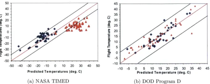
1-5 Comparison of flight data to temperature predictions for two spacecraft

1-6 Comparison of flight data to model predictions for seven GSFC missions

1-7 ISS Heat Rejection System radiator . . . .

1-8 UQ toward validating system performance with respect to QoI . . . . 1-9 General global sensitivity analysis process . . . . 1-10 Comparison of model-based DOE methods . . . . 1-11 Thesis roadm ap . . . .

2-1 BMV methodology overview . . . . 2-2 Mapping of physical problem, conceptual model, and simulation model

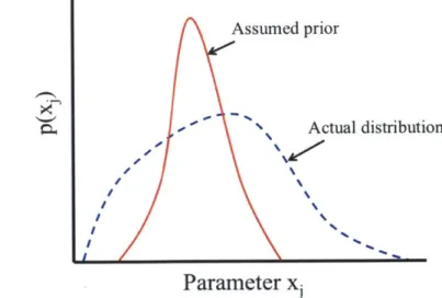
2-3 Notional variances of parameter uncertainty distribution . . . .

2-4 BMV experimental goal setting . . . .

3-1 3-2 3-3 3-4 3-5 3-6 28 30 33 35 39 40 43 . . 48 51 56 . . 68 70 72 74 78 Physical problem for radiator case study . . . . Conceptual model for radiator case study . . . . Notional uniform distribution . . . . Preliminary uncertainty analysis results for radiator . . . . Local sensitivity analysis for isothermal radiator . . . . Preliminary global sensitivity analysis results for radiator . . . 4 . . . . 91 . . . . 91 . . . . 93 . . . . 95 . . . . 96 . . . . 97

3-7 Experimental utility, U(d), contour plot of possible experiments . . . . 101

3-8 High fidelity Thermal Desktop radiator model . . . . 102

3-9 Thermal Desktop model solution for parameter inference experiment . . . . . 103

3-10 Model calibration results for radiator coating emissivity . . . . 104

3-11 Contour plot of the joint distribution of

#

and e . . . . 105

3-12 Uncertainty propagation results for radiator; updated coating emissivity . . . 107

3-13 Model discrepancy distributions from model validation experiment . . . . 110

3-14 Uncertainty analysis results following model validation experiment . . . . 111

3-15 Sensitivity analysis of heat flux, q, for radiator . . . . 114

3-16 Thermal Desktop results for thermal balance test . . . . 118

3-17 Model predictions of radiator temperature versus heat load . . . . 119

3-18 Timeline of BMV and conventional validation process . . . . 122

3-19 Illustration of BMV on general system over project lifecycle . . . . 123

4-1 Spectrometer design overview . . . . 127

4-2 SXM design overview . . . . 128

4-3 Isometric and side views of REXIS instrument on OSIRIS-REx . . . . 129

4-4 Solar distance versus mission time for entire 7-year mission . . . . 129

4-5 Temperatures of Bennu plotted versus longitude and latitude . . . . 131

4-6 Amptek AXR SDD package . . . . 134

5-1 Nominal thermal predictions for SXM . . . . 144

5-2 Joint cumulative distribution function for Tdd and TO-REX . . . . 146

5-3 Histograms and CDFs of T,8 conditioned on TO-REX . . . . -. 148

5-4 Probability of satisfying SXM requirements versus TO-REx . . . . 149

5-5 Main effects global parameter sensitivities of SXM model . . . . 151

5-6 Convergence plot for experimental utility, U(d) . . . . 158

5-7 Histogram of experimental utilities and scatter plots of utilities . . . . 160

5-8 Heatmap of experimental utility for TO-REx versus VTEC . . . . . . . 161

5-9 SXM sensor correlation coefficients . . . . 163

5-11 5-12 5-13 5-14 5-15 5-16

T.9d versus VTEC various interface temperatures . . . . Tqddversus iTEC for various interface temperatures . . . . Comparison of Amptek performance estimates with SXM TEC data . . .

Tsdd versus TEC power dissipation for various interface temperatures

Temperature difference between the SDD housing and SXM interface Temperature difference between the SDD housing and the SXM housing.

5-17 Surface fit for SDD temperature for various VTEC and Th . . . . .

5-18 Surface fit for the TEC current draw for various VTEC and Th . . 5-19 Model calibration process overview . . . . 5-20 Notional prior or posterior predictive check . . . . 5-21 Prior predictive check for test phase T36; Gh . . . .

5-22 Prior predictive check for test phase T36; Gh and G,,b . . . .

5-23 Bottom view of SXM housing . . . . 5-24 Prior predictive check for test phase T36; Gh and G,,b relaxed 5-25 Prior predictive check for test phase T36; Gh, G,,b relaxed, Gb

5-26 Plot of adaptive MCMC chain pushing up against the upper limit 5-27

5-28 5-29

of Gh.

Intermediate posterior histograms and scatterplots for calibration parameters Plot of adaptive MCMC chain showing good mixing after initial burn-in. . . Final posterior histograms and scatterplots for calibration parameters . . . . 5-30 Posterior predictive check for test phase T36

5-31 5-32 5-33 5-34 5-35 5-36 5-37 5-38

Posterior predictive check for all 43 test phases . . . . Comparison of GP training points and predictions . . . .

GP model section for bracket model discrepancy . . . . GP model section for SDD housing model discrepancy . . . . SDD discrepancy samples and histogram . . . .

Posterior predictive check for test phase T36, both with/without 6(x) Probability of satisfying SXM requirements versus TO-REX . . . . Illustration of BMV on REXIS SXM over project lifecycle . . . .

A-1 SXM structure and component overview . . . .

166 167 168 169 170 171 175 175 176 177 180 182 184 185 187 191 192 193 194 . . . . 195 . . . . 196 . . . . 200 . . . . 202 . . . . 203 . . . . 204 . . . . 206 - . . . 210 .... 216 239

A-2 Top view of SXM interface plate ...

A-3 SXM structure showing RTD on SDD housing . . . .

A-4 SXM structure with all SXM RTDs . . . . A-5 Final view of SXM test article with MLI blanket . . . . A-6 SXM test grid ...

A-7 SSL thermal vacuum chamber ...

A-8 Notional SXM thermal test electronics/control configuration A-9 SXM RTD placement ...

A-10 Model predictions for the mission Cruise Phase cold case . . A-11 Model predictions for the mission operational hot case . . .

C-1 C-2 C-3 C-4 C-5 C-6 C-7 . . . 240 . . . . 241 . . . 241 . . . . 242 . . . . 245 . . . 248 . . . . .. . . . 249 . . . . 250 . . . 253 . . . 254 Lumped parameter concept . . . .

ID mesh with uniform discretization . . . . SDD temperature versus voltage for SXM TEC . . . . . SDD temperature versus current for SXM TEC . . . . . Applied voltage versus current draw for SXM TEC . . . SXM node assignments for the lumped parameter model Connectivity matrix for SXM model . . . .

266 268 270 271 272 273 274 275 278 C-8 Notional SXM MLI heat flow diagrams of the MLI outer cover

List of Tables

1.1 Spacecraft thermal control component examples . . . . 26

1.2 Summary of flight thermal statistical data . . . . 38

1.3 Nominal values for sample radiator calculation . ... . . . . 42

1.4 Examples of environmental test condition guidance . . . . 59

1.5 Comparison of state of the art and conventional methods . . . . 65

2.1 Observability for parameter inference experiment . . . . 83

3.1 Nominal parameter values for sample radiator problem thermal model . . . . 92

3.2 Initial parameter uncertainty characterization . . . . 93

3.3 Experimental conditions for model validation experiment . . . . 109

3.4 Summary of uncertainty analysis results . . . . 112

3.5 Initial model parameters for conventional analysis of radiator . . . . 116

3.6 Final parameters for conventional analysis of the radiator . . . . 120

4.1 Summary of REXIS thermal analysis cases . . . . 132

4.2 SXM steady state component temperature limits . . . . 133

5.1 Temperature limits for validation requirements . . . . 138

5.2 SXM model nominal parameter values . . . . 140

5.3 SXM model parameter prior uncertainty distributions . . . . 142

5.4 Thermal conductance design guidelines . . . . 143

5.5 Table of SXM parameter inference experimental conditions . . . . 155

5.7 GP model hyperparameter regressed values . . . . A.1 A.2 A.3 A.4 A.5

SXM component temperature limits . . . . Personnel schedule for monitoring test chamber . . . . . List of RTDs for thermal test . . . . SXM survival temperature limits . . . ... . . . . SXM operational temperature limits . . . .

. . . 199 . . . 243 . . . 244 . . . 251 . . . 255 . . . 255 B.1 Stabilized RTD readings for test phases T1 through T43

B.2 Temperature of SDD for test phases T1 through T43 . . C.1 Parameter values for SXM MLI sensitivity analysis . . .

262 263 276

Glossary

aleatory uncertainty: model uncertainty due to intrinsic randomness [55]

complex system: a system with global emergent dynamics resulting from its many

interact-ing elements [18]

epistemic uncertainty: model uncertainty due to lack of knowledge [55]

model calibration: the use of experimental observations of a physical system to learn about

the parameters of the model [26, 27]

model correlation: the process where one gains modeling insight by observing differences in

comparable quantities between model and test [26, 27]

model inadequacy: the inherent inability of the model to reproduce reality [60]

model validation: process of confirming a model is an adequate representation of the physical

system and is capable of predicting the systems behavior accurately with respect to the require-ments within the domain of the intended application of the model [20, 21]

model verification: process of ensuring the model implementation represents the conceptual

description of the model and the model's solution [20, 21]

parameter: a quantity that determines the characteristics of a model, including external inputs to the model that are not contained in the system model itself

sensitivity analysis: the determination of how a model's parametric uncertainties contribute to its output uncertainty [43]

simulation model: mathematical representation of a conceptualized model of the real system through which model parameters and operations yield predictions for the physical response of the

system

thermal balance test: dedicated test phases simulating flight conditions to gather steady state temperature predictions to verify that the thermal control system meets requirements and correlate

thermal models [4, 22, 24]

thermal system: system responsible for maintaining all system component temperatures within allowable limits for all modes of operation over the entire domain of relevant mission environments

[4, 5]

thermal vacuum test: performance verification of spacecraft components through functional testing during a number of hot and cold cycles at prescribed test levels in vacuum [4, 22, 24]

uncertainty analysis: the determination of a model's output uncertainty due to its uncertain parameters and its inadequacy [41]

uncertainty quantification: the quantitative characterization and reduction of uncertainty, in-cluding forward uncertainty propagation (forward problem) and model calibration (inverse problem)

Nomenclature

Mathematical Definitions:

E[.] = expectation

Q

= Quantities of Interest (QoI)

R = correlation coefficient

SLj = local sensitivity for jth parameter

Si = main effect global sensitivity for Jh parameter

STj = total effect global sensitivity for jth parameter

U(.) = utility V[-] = variance d = experimental conditions p(.) = probability density x = model parameters y = model output z = experimental data/observations 7 = calibration parameters 6(.) = model discrepancy

= true physical process

= simulation model mapping parameters to output 6 = experimental parameters of interest

A = Gaussian Process characteristic length

p = mean value

-= standard deviation

-o = Gaussian Process output variance

Physical Definitions:

A = surface area

C = heat capacity

Kp = control gain

Q

= heat load R = electrical resistance Rt = thermal resistance T = temperature V = voltage C= specific heat e = process error i = current k = conductivity m =mass q = heat flux t = time a = absorptivity = emissivity

C* = multi-layer insulation (MLI) blanket effective emissivity

em = observation error

0 = incidence angle

p = density

o- = Stefan-Boltzmann constant

Chapter 1

Introduction

This chapter provides introductory material for this research. Section 1.1 is a thesis primer, Section 1.2 provides background information, and Section 1.3 explains the motivation for the work. Section 1.4 reviews the current relevant literature in the area of model validation, and Section 1.5 shows the thesis objectives for this research. Finally, the thesis roadmap is given in Section 1.6.

1.1

Thesis Primer

The scope of space-based missions is significantly driven by cost. The cost of a particular mission is highly correlated to its resource consumption (e.g., mass or volume). Further-more, resource-related costs are incurred both on the system itself and the launch vehicle. For example, the NASA and Air Force Cost Model (NAFCOM) [1] is a parametric cost esti-mation model based on historical data from previous space projects. In NAFCOM, mass is a significant cost driver in the subsystem-level parametric equations. Massive and/or volumi-nous spacecraft require large, expensive rockets to reach orbit. Launch vehicle costs persist as a significant contributor to overall mission cost. Despite the promise of next-generation launch vehicles, today we are limited to costs ranging from $2,000 to $10,000 per pound to low-Earth orbit [2, 3]. Process costs (e.g., system analyses, technology development, and verification and validation) are also highly correlated to mission costs. The time and orga-nizational resources needed to develop and operate a system comprise a- significant portion

of overall mission cost. Because simulation model predictions are used to allocate system resources and develop a system over the entire project lifecycle, it is important to achieve high confidence in spacecraft simulation models as early as possible. An improvement to the model validation process means not only improving the form of the system post-validation but the processes associated with model validation itself.

In spacecraft design, thermal control systems are developed throughout the project life-cycle and can significantly impact spacecraft form-related and process-related cost. This research focuses on improving the model validation process for spacecraft thermal systems. Thermal systems are primarily responsible for maintaining all system component tempera-tures within allowable limits for all modes of operation over the entire domain of relevant mission environments [4, 5]. Thermal models are used to predict performance (usually tem-peratures and heat flows) of the thermal system during flight. Based on these predictions, system resources, including power, volume, and mass, are allocated to satisfy requirements. This research introduces a Bayesian-based Model Validation (BMV) methodology to improve the model validation process for spacecraft thermal systems. BMV combines the methodologies from the fields of Uncertainty Quantification (UQ) and Design of Experiments (DOE) to validate thermal models. The BMV methodology was developed with the long term goal of improving the accuracy of on-orbit predictions, making the model validation process more rigorous and systematic in addressing model uncertainties, and decreasing the resources required to meet thermal system requirements. BMV is implemented in two case studies: a passive spacecraft radiator and on the REgolith X-ray Imaging Spectrometer

(REXIS) instrument solar X-ray monitor (SXM).

1.2

Background

This section introduces background information for the validation of thermal simulation models. First, an overview of thermal system engineering is discussed to examine typical de-sign practices and conventions. Next, a description of thermal simulation models is provided. Finally, the treatment of model uncertainty and simulation model validation is presented in a general format to introduce how complex models are developed throughout the project

lifecycle.

1.2.1

Thermal System Engineering

Thermal system engineering begins early in a project's lifecycle with preliminary design and analysis efforts. The early stage of design is critical because it is when the design concept develops. As the system concept matures, thermal engineers take inputs from other disciplines (e.g., structures and avionics) to develop a preliminary design. Simple analysis models are used to evaluate feasibility and allocate resources to the thermal system. As the design matures, high fidelity models are developed to predict the response of the system to its mission environments. The models are correlated with results from thermal testing to produce the final mission temperature predictions. [4, 5]

There are two main thermal control component classifications for spacecraft: active and passive. Active control systems regulate the thermal behavior of a component or subsystem by monitoring its behavior and providing control when required. Passive thermal control sys-tems regulate the physical response of the system via static design elements such as material properties, coatings, and multi-layer insulation (MLI) blankets. Passive components cannot be changed once on-orbit and do not adapt to system or thermal environment conditions to provide thermal control. The selection of active and passive components is system-specific

and depends on the thermal system requirements and configuration. For example, although passive control elements can have lower mass and cost [4], active thermal control compo-nents can have significant analysis or system performance benefits (e.g., louvers can decrease heater power).

Components selected for thermal control vary widely, ranging from those used to iso-late certain components in conduction and radiation to those used to directly transfer heat within the system. Table 1.1 illustrates the spectrum of thermal control components avail-able to engineers when designing a thermal system. The design spectrum includes compo-nents commonly implemented on satellites [4, 6] and emerging thermal technologies (e.g., electrochromics) [7]. The components in Table 1.1 are divided into the active and passive control categories and are further subdivided by how the component is typically used within the system: for isolation, heat transfer, or heat rejection to deep space (radiators). For

example, a thermal strap is a passive heat transport component used to conduct heat from a source to a sink, whereas a fluid loop is an active component that uses the fluid to transfer heat to different parts of the system. In order to achieve a thermal design, engineers select surface finishes and components to facilitate the desired heat transfer. At the most basic level, thermal design consists of sizing radiators for the hottest environments and sizing heaters for the coldest environments [8]. Radiators reject unwanted waste heat to space, and heaters are strategically placed on components and powered by the spacecraft to warm components that are nominally too cold. Generally, thermal systems are cold-biased because it is physically easier and more reliable to warm than cool components.

Table 1.1: Spacecraft thermal control component examples

Isolation

Mult-layer Insulation Lmatw

Heat

Transport

Bet Pie Therea Strap Ma pod

HdA Het Exchafger

Radiators

tuctral radiator &ody-inounted _______ RUN___"

1.2.2

Thermal Simulation Models

Feasibility studies and analyses begin as soon as preliminary designs are established through the use of thermal simulation models. A simulation model is a mathematical representation of a conceptualized model of the real system through which model parameters and operations yield predictions for the physical response of the system. The goal of thermal models is to estimate the solution to the general heat transfer equation, as shown in Equation (1.1):

aT

PCp = V - k(V -T) + Q(T, t) (1.1)

where p is density, c, is specific heat, k is the conductivity tensor, Q(Tt) is the source heat term, t is time, and T=T(xy,zt) is the spatial and temporal temperature variation. The initial conditions and boundary conditions are needed to fully solve Equation (1.1). Model parameters are quantities that determine the characteristics of the model, including external inputs to the model that are not contained in the system model itself (e.g., solar flux or thermal resistance between two components). Parameters include geometries of the system, component connectivity, and material properties that map to the k, p, and c, terms.

Both conduction and thermal radiation are captured in Equation (1.1). The V -k(V -T) term captures the conduction through the system. Q(Tt) is both the heat transfer within the system and the heat transfer between the system and its environment. Components of

Q(T,t) can be categorized as shown in Equation (1.2) [9]:

Q(T, t)

= Qext + Qpow + Qrad (1.2)

where Qext captures external heating,

Q,,

is the power dissipations of components, and Qrad is radiation within the system. The terms

Q,,,

and Qrad represent physics associated with the model itself. Radiation within the system is a function of the geometry. For example, the view factor from one surface to another directly affects the radiation heat transfer between the surfaces. Qext refers to the heat fluxes imposed onto the system by the space thermal environment. Although a given space mission is exposed to a thermal environment that yields unique external heating factors, there is a general thermal environment that applies to most spacecraft, as shown in Figure 1-1. Heat inputs come from three major sources: direct sunlight, radiation in the infrared spectrum from nearby planetary bodies (e.g., a planet or an asteroid), and sunlight reflected by nearby planetary bodies (i.e., albedo). The primary method of heat rejection for spacecraft is radiation to deep space. Often, Qext is given by Equation (1.3):

where the heat fluxes are Qsoiar due to direct sunlight, QIR due to light in the infrared

spectrum from a nearby planetary body, and Qalbed, due to reflected, or albedo, light from a nearby planetary body. Given the thermal environment, component power dissipations, and system geometry parameters, Q(Tt) is completely specified. Once all parameters, initial conditions, and boundary conditions are defined, the solution to Equation (1.1) for the system can be approximated via thermal model(s).

Spacecraft Sun

Solar Radiation

Albedo diationto_space

ared

Planetary Body

Figure 1-1: Spacecraft thermal environment [4]. In general, there can be multiple planetary bodies (e.g., an asteroid and a planet).

The fidelity of thermal models depends on the accuracy required of the model (derived from the requirements) and the thermal system complexity. Fidelity of the models often increases over the project lifecycle as design details emerge. Early in the design life cycle, preliminary analytical models [10] and lumped parameter models [11, 12] are used to evaluate system concepts, define thermal interfaces, and identify critical sensitivities. Preliminary models explore the feasibility of early designs and their impact on system resources. Because the system is immature, accounting for important model uncertainties (e.g., component power dissipations) is critical for ensuring conservative analyses. Experience and engineering judgment determine how the preliminary models are used and when to transition to higher fidelity models. Higher fidelity modeling is almost exclusively performed by commercially available software packages that offer state of the art techniques to numerically approximate the solution to Equation (1.1) [13]. While finite element methods are sometimes used [4],

the most commonly used commercial thermal model computer code is the finite difference code SINDA [14]. SINDA is commonly interfaced through the NASA standard Thermal Synthesizer System [15] or Thermal Desktop [13, 16]. Nearly all thermal models, regardless of the model fidelity and software used, generate predictions based on the parameters and mission environment.

1.2.3

Traditional Treatment of Model Uncertainty

Model uncertainty is uncertainty in aspects of a simulation model that results in uncertainty in the model's predictions. Parametric uncertainties are those uncertainties associated with not knowing the true model parameter values. Model structure uncertainties result in model error due to limitations with how the physical processes within the system are modeled (e.g., omitted physics, discretization of components or interfaces, or simplifying assump-tions). Uncertainty quantification (UQ) is the quantitative characterization and reduction of uncertainty, including forward uncertainty propagation and model calibration [17]. Com-plete UQ requires quantification of parametric and model structure uncertainties. UQ is critical for model validation because the accuracy of a model in predicting the behavior of a physical system depends on the model's uncertainty.

Currently, a complete quantification of model uncertainties is typically not performed in the development of spacecraft thermal systems. Thermal systems are considered complex systems, which are systems with global emergent dynamics resulting from its many interact-ing elements [18]. The model development process of a typical complex system is depicted in Figure 1-2 [19]. A serial progression is shown, but the dashed arrows indicate that the model development processes often occur in parallel. First, the model is built based on the design of the real world system. Once the model is built, verification and validation ensure that the model was built to correctly, is in accordance with its intended purpose, and can adequately predict the real system's behavior. Once the model is finished, the remaining model uncertainties are quantified, and then the model is put into application. In most cases, uncertainties are not quantified upstream of a model. Instead, uncertainty margins are often applied to model output (i.e., downstream of the model) based on design standards and expert opinion [8] to account for unquantified parametric and model structure uncertainties.

Although not common, uncertainties are sometimes captured upstream of the model and are propagated through the model to the output. Even when uncertainties are captured upstream, uncertainty quantification usually focuses on parametric model uncertainties and does not address model structure uncertainties. The neglect of model structure uncertainties can cause important discrepancies between the model and the physical system. A systematic procedure for addressing model uncertainties upstream of the model is needed to improve the development process in Figure 1-2.

Real Wold System Model Building - -Model Vernfication Model Validation Model Model

Figure 1-2: Typical model development process for a complex system. Figure modified from [19, Fig. 1-2].

1.2.4

Model Validation

Model "correctness" is addressed through verification and validation [20]. Model verification is the process of ensuring that the model implementation is consistent with the model's output and represents the conceptual description of the model. Model validation is the process of confirming a model is an adequate representation of the physical system and is capable of predicting the systems behavior accurately with respect to the requirements within the domain of the intended application of the model [20, 21]. It is generally not possible to prove a simulation code correct [21], but industry standard software packages (e.g., SINDA and Thermal Desktop) are verified to a high confidence level before being put into use. The verification of a specific model's implementation is primarily achieved through experience,

expert review, and a comparison with analytical solutions [20]. Once the model is deemed a faithful representation of what was intended, verification is complete and validation becomes the primary focus. The focus of this research is on improving the model validation process and quantifying the uncertainties associated with the validated model's output.

In the development of spacecraft thermal systems, rules and guidelines are in place to verify the system design and validate the models. Guidance includes processes for thermal model development and testing (at prototype, subsystem, and system level) for both military programs [22, 23] and NASA Goddard programs [24, 25]. Analyses focus on worst-case scenarios that are built for the hottest and coldest thermal environments in each mission phase. Thermal design margins are applied directly to the worst-case temperature predictions to account for model uncertainty. Design margins are consistent with Figure 1-2 because they are applied downstream of the model and account for both parametric and model structure uncertainties. For passive systems, military programs apply a recommended 17 'C margin (which may be reduced to 11 'C after model validation) [22] and many NASA programs must demonstrate a 5 'C margin [25] (though can be raised to 10 *C based on the specific application [8]). For active thermal control elements, heat load margin may be used in lieu of temperature margin.

The guiding philosophy for design verification testing is "test like you fly, and fly like you test" [25]. Testing in an evacuated chamber with heat sources to emulate mission envi-ronment fluxes is considered the best possible simulation of the space thermal envienvi-ronment. Thermal vacuum and balance tests are commonly used experimental techniques to validate a thermal system design and model. Thermal vacuum testing is performance verification of spacecraft components through functional testing during a number of hot and cold cycles at prescribed test levels. Thermal balance tests are dedicated test phases simulating flight con-ditions to gather steady state temperature predictions to verify the thermal control system and correlate thermal models [4, 22, 24]. From experimental data, models are calibrated and correlated. Model calibration is the use of experimental observations of a physical system to learn about the parameters of the model; model correlation is the process to gain model insights by observing differences in comparable quantities between model and test [26, 27].

and predict that requirements are met with adequate margin. If correlated models predict that requirements are not satisfied, additional resources can be allocated (e.g., radiators made larger) to achieve required temperatures with margin. A design change late in the project lifecycle due to unexpected thermal system performance during testing (e.g., power dissipations significantly larger than expected) is expensive and can have significant schedule impacts.

1.3

Motivation

Long term, improving the spacecraft thermal model validation process can result in a re-duction in form-related and process-related mission costs. This section will first discuss why the thermal system is an important component of a spacecraft's overall cost. Significant mission costs are associated with the form of the spacecraft and processes involved in its development. Next, evidence is presented that suggests current model validation practices can result in overly conservative on-orbit predictions [8, 28, 29, 30, 31]. As a result of the conservatism, thermal systems are intentionally overdesigned and consume additional mass, volume, and power. Furthermore, model inaccuracies are seen in some systems where a conventional model validation process did not reveal inadequacies with the model, analyses, and/or testing. This section will conclude by introducing and answering model validation evaluation questions to determine the effectiveness of current validation practices.

1.3.1

Mission Costs Associated with Thermal Systems

Reductions in mission costs associated with the system's resource consumption (i.e., form) and processes required to develop the spacecraft are possible by improving the thermal model validation process. The goal of this section is to explain the coupling between thermal systems and mission costs. Form-related costs are discussed first, followed by a discussion of process-related costs.

Often, thermal systems are thought to not drive the consumption of spacecraft resources relative to other systems (e.g., structures). Consequently, resource consumption reduction efforts (e.g., design optimization to minimize mass) tend to focus less on thermal systems

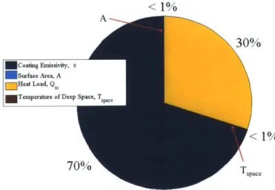
compared to other systems. As an example of how the thermal system impacts resources at the spacecraft level, Figure 1-3 shows the results of a study [32] that examined the composi-tion of an average spacecraft's mass. The study found that the thermal system can comprise approximately six percent of a spacecraft's dry mass. The study in Figure 1-3 contains data from diverse mission types, including the Global Positioning System, communications satel-lites, and science missions. At face value, statistics such as those shown in Figure 1-3 seem to indicate that thermal systems are of second-order importance with respect to a spacecraft's overall resources (in this case mass is shown but similar statistics can be shown for power and volume). However, there can be significant physical couplings between the thermal sys-tem and other spacecraft syssys-tems (i.e., syssys-tems are not independent). Although Figure 1-3 shows that six percent of mass is only thermal system mass, there is mass that exists in other portions of the pie chart for thermal reasons. For example, a spacecraft bus structure receives design inputs from thermal analysis and also serves as a primary mechanism for heat transfer within a system. A component can be both a structural element and a significant thermal path of a spacecraft [9]. The thermal system's impact on spacecraft resources can be larger than six percent when considering the interconnectivity to other spacecraft systems.

Figure 1-3: Dry mass distribution of an average earth-orbiting spacecraft. Figure from [32, Fig. 1].

Furthermore, system-specific factors such as those systems with significant thermal con-trol challenges, those that are highly resource-constrained systems, and those that carry large uncertainty margins due to risk aversion are not captured in Figure 1-3. Such systems

often require more resources to achieve thermal requirements. For example, the James Webb Space Telescope (JWST) sun shield, only a portion of the thermal system, is approximately 12 percent of the total system mass and must be deployed in the space environment because its volume is too big to be open in the launch vehicle fairing [33]. Thermal control drives the JWST system design. For highly resource constrained systems (e.g., small satellites or payload instruments), small decreases in resource consumption are very beneficial because the power, volume, and mass budgets are very restrictive. Although the thermal system may comprise a small portion of the overall resources, design to minimize a resource on a highly resource constrained system (e.g., volume of instrument radiator) should not be overlooked. The REXIS instrument, discussed in Chapter 4, is an example of a resource-constrained instrument.

The TIRS instrument on the Landsat Data Continuity Mission [34] is a recent exam-ple of how thermal model validation can affect cost associated with resource consumption. On TIRS, an aggressive schedule, a need to procure long-lead items early, and large heat load uncertainties led to a risk reduction philosophy that emphasized large thermal design margins. In particular, the TIRS thermal team devoted significant efforts to character-izing the heat loads into the cryogenic subsystem via analysis, hand calculations, and a complex prototype-level test'. Once the flight design was tested in thermal vacuum, better-than-expected-performance of the cryocooler led to considerable margin on the cryocooler radiator. Before launch, ;60% of the radiator's surface area was covered with MLI blankets to ensure that components did not violate minimum temperature limits, as shown in Figure 1-4. The excess cryocooler radiator surface area on TIRS is not only increased mass, volume, and heater power attributed to the thermal system, but the effect of the excess resources propagates through to the resources used by other subsystems (e.g., the TIRS structure must support a radiator with significantly larger mass than is needed). Reduction in the resource consumption of thermal systems is an important component of reducing a spacecraft's overall use of mass, power, and volume and thus, reducing form-related costs.

Although form-related mission costs are sometimes easier to quantify, process-related costs can be just as, if not more, significant. Process cost refers to the cost associated with

Figure 1-4: TIRS instrument radiator with multi-layer insulation blankets covering ~60% of radiator surface area [35]

spacecraft development and operation such as technology development, system analyses, system verification and validation, and on-orbit mission control operations. To illustrate the significance of anticipated process-related costs for an interplanetary mission, the operations and data analysis costs comprised approximately $175 million of the $680 million budget of the Mars Reconnaissance Orbiter [36]-a significant portion of the overall MRO mission budget. Model-based design and model validation play an important role in spacecraft development and operation processes and can adversely affect missions when performed inadequately.

For example, insufficient instrument-level thermal model validation led to high process-related costs on the Juno mission immediately after launch. Juno was launched in 2011 and is an interplanetary mission that accomplishes its science objectives in a polar orbit about Jupiter [37]. Soon after launch, two payload instruments began encountering warmer temperatures than expected. A conventional model validation approach did not reveal inad-equacies with the thermal model, analyses, thermal balance testing, and communication of results. Extensive analyses and test efforts were made after launch to detect and mitigate

the problem. Janis Chodas, Juno Project Manager, stated2:

"An improved understanding of the Juno instruments' thermal interactions with the space-craft, and better instrument thermal model validation, would have decreased the amount of post-launch investigative work that the Juno team had to do when some instruments encoun-tered thermal problems inflight."

The instrument problems incurred during the Juno mission are just one example of the im-portance of model validation in the context of process costs. An improvement to the model validation process can result in not only reducing form-related costs but also a reduction in process-related costs, which can be just as if not more significant.

1.3.2

Evaluation of Current Thermal Model Validation

Given the high demand for mission success and resource efficiency, it is prudent to once again review model validation practices for current systems [38]. While Section 1.2 provides high-level information and context for the thermal model validation process, we are left with the question: how effective are current thermal model validation practices? Since model validation requires a comparison of the modeling world with the real world, we can evaluate our validation processes by looking at final thermal model predictions versus actual flight data. The following model validation evaluation questions arise:

" How close are post-validation model predictions and flight temperature data?

" Are there trends in the model predictions and/or data that suggest an opportunity to improve the validation process?

" Are design uncertainty margins appropriately conservative? Is there a better way to quantify and reduce the uncertainty?

" Why buck the status quo?

The comparisons of thermal model predictions and flight data lead to answers for each question. The answer to each is shown in Section 1.3.4.

Current thermal model validation practices, relatively unchanged over several decades, have a long history of leading to successful space missions. However, a comparison of on-orbit temperature data and model predictions reveals limitations with the validation process. In the late 1960-70s, initial comparisons were made between thermal model predictions, thermal vacuum test data, and flight temperatures [30, 31]. Results showed that by correlating a model to test results, the standard deviation to flight data reduced from 9 "C to 5.6 'C [28]. Based on these early examinations of correlated models and flight data, the temperature margins currently in place for military programs (see Section 1.2.4) were adopted.

In 2006, Welch [28] sought to revisit the military standards [22, 23] established in the 1970s by looking at more recent programs. Thermal model predictions and on-orbit tem-perature data from different space programs were analyzed statistically. The study includes spacecraft from DOD programs, ESA programs, an Iridium satellite, and the NASA Ther-mosphere Ionosphere Mesosphere Energetics and Dynamic (TIMED) mission. The results of the study are shown in Table 1.2. The second column in the table indicates the mean difference between the model predictions and temperature data, plus/minus two standard deviations. The third column shows the derived thermal uncertainty margin to capture 95% of the flight temperatures and model prediction discrepancies. The third column is derived from the second column. DOD Programs A and B are programs from the 1980s and serve as a basis for comparison to the more recent programs shown.

The main takeaway from Table 1.2 is that the data suggest that the thermal models are not accurately predicting the flight temperatures for all missions. The derived thermal uncertainty margin refers to the error bounds on the mean of the predictions required to capture the flight temperatures. On average, the derived uncertainty margin to meet the 95% threshold is above 10 *C. For some programs, exceeding a derived uncertainty margin of 10 *C was due to a mean that was far from zero (e.g., NASA TIMED) and for others it was due to a large variance about a near-zero mean (e.g., DOD Program D). Between DOD Programs A and B and more recent missions (from the late 1990s and early 2000s), there is no obvious accuracy improvement even though modeling software tools have greatly improved