EUROPEAN ORGANIZATION FOR NUCLEAR RESEARCH (CERN)
CERN-LHCb-DP-2013-002 February 13, 2015
Measurement of the track
reconstruction efficiency at LHCb
The LHCb collaboration†
Abstract
The determination of track reconstruction efficiencies at LHCb using J/ψ → µ+µ− decays is presented. Efficiencies above 95% are found for the data taking periods in 2010, 2011, and 2012. The ratio of the track reconstruction efficiency of muons in data and simulation is compatible with unity and measured with an uncertainty of 0.8 % for data taking in 2010, and at a precision of 0.4 % for data taking in 2011 and 2012. For hadrons an additional 1.4 % uncertainty due to material interactions is assumed. This result is crucial for accurate cross section and branching fraction measurements in LHCb.
Published in JINST 10 (2015) P02007 c
CERN on behalf of the LHCb collaboration, license CC-BY-3.0.
†Authors are listed on the following pages.
LHCb collaboration
R. Aaij41, B. Adeva37, M. Adinolfi46, A. Affolder52, Z. Ajaltouni5, S. Akar6, J. Albrecht9, F. Alessio38, M. Alexander51, S. Ali41, G. Alkhazov30, P. Alvarez Cartelle37, A.A. Alves Jr25,38, S. Amato2, S. Amerio22, Y. Amhis7, L. An3, L. Anderlini17,g, J. Anderson40, R. Andreassen57, M. Andreotti16,f, J.E. Andrews58, R.B. Appleby54, O. Aquines Gutierrez10, F. Archilli38, A. Artamonov35, M. Artuso59, E. Aslanides6, G. Auriemma25,n, M. Baalouch5, S. Bachmann11, J.J. Back48, A. Badalov36, W. Baldini16, R.J. Barlow54, C. Barschel38, S. Barsuk7, W. Barter47, V. Batozskaya28, V. Battista39, A. Bay39, L. Beaucourt4, J. Beddow51, F. Bedeschi23,
I. Bediaga1, S. Belogurov31, K. Belous35, I. Belyaev31, E. Ben-Haim8, G. Bencivenni18, S. Benson38, J. Benton46, A. Berezhnoy32, R. Bernet40, M.-O. Bettler47, M. van Beuzekom41, A. Bien11, S. Bifani45, T. Bird54, A. Bizzeti17,i, P.M. Bjørnstad54, T. Blake48, F. Blanc39, J. Blouw10, S. Blusk59, V. Bocci25, A. Bondar34, N. Bondar30,38, W. Bonivento15,38, S. Borghi54, A. Borgia59, M. Borsato7, T.J.V. Bowcock52, E. Bowen40, C. Bozzi16, T. Brambach9,
J. van den Brand42, J. Bressieux39, D. Brett54, M. Britsch10, T. Britton59, J. Brodzicka54, N.H. Brook46, H. Brown52, A. Bursche40, G. Busetto22,r, J. Buytaert38, S. Cadeddu15, R. Calabrese16,f, M. Calvi20,k, M. Calvo Gomez36,p, P. Campana18,38, D. Campora Perez38, A. Carbone14,d, G. Carboni24,l, R. Cardinale19,38,j, A. Cardini15, L. Carson50,
K. Carvalho Akiba2, G. Casse52, L. Cassina20, L. Castillo Garcia38, M. Cattaneo38, Ch. Cauet9, R. Cenci58, M. Charles8, Ph. Charpentier38, S. Chen54, S.-F. Cheung55, N. Chiapolini40, M. Chrzaszcz40,26, K. Ciba38, X. Cid Vidal38, G. Ciezarek53, P.E.L. Clarke50, M. Clemencic38, H.V. Cliff47, J. Closier38, V. Coco38, J. Cogan6, E. Cogneras5, P. Collins38,
A. Comerma-Montells11, A. Contu15, A. Cook46, M. Coombes46, S. Coquereau8, G. Corti38, M. Corvo16,f, I. Counts56, B. Couturier38, G.A. Cowan50, D.C. Craik48, M. Cruz Torres60, S. Cunliffe53, R. Currie50, C. D’Ambrosio38, J. Dalseno46, P. David8, P.N.Y. David41, A. Davis57, K. De Bruyn41, S. De Capua54, M. De Cian11, J.M. De Miranda1, L. De Paula2, W. De Silva57, P. De Simone18, D. Decamp4, M. Deckenhoff9, L. Del Buono8, N. D´el´eage4, D. Derkach55, O. Deschamps5, F. Dettori38, A. Di Canto38, H. Dijkstra38, S. Donleavy52, F. Dordei11, M. Dorigo39, A. Dosil Su´arez37, D. Dossett48, A. Dovbnya43, K. Dreimanis52, G. Dujany54, F. Dupertuis39, P. Durante38, R. Dzhelyadin35, A. Dziurda26, A. Dzyuba30, S. Easo49,38, U. Egede53, V. Egorychev31, S. Eidelman34, S. Eisenhardt50, U. Eitschberger9, R. Ekelhof9, L. Eklund51, I. El Rifai5, Ch. Elsasser40, S. Ely59, S. Esen11, H.-M. Evans47, T. Evans55, A. Falabella14, C. F¨arber11, C. Farinelli41, N. Farley45, S. Farry52, RF Fay52, D. Ferguson50, V. Fernandez Albor37, F. Ferreira Rodrigues1, M. Ferro-Luzzi38, S. Filippov33, M. Fiore16,f, M. Fiorini16,f, M. Firlej27, C. Fitzpatrick39, T. Fiutowski27, M. Fontana10, F. Fontanelli19,j, R. Forty38, O. Francisco2, M. Frank38, C. Frei38, M. Frosini17,38,g, J. Fu21,38, E. Furfaro24,l, A. Gallas Torreira37, D. Galli14,d, S. Gallorini22, S. Gambetta19,j, M. Gandelman2, P. Gandini59, Y. Gao3, J. Garc´ıa Pardi˜nas37, J. Garofoli59, J. Garra Tico47, L. Garrido36, C. Gaspar38, R. Gauld55, L. Gavardi9, G. Gavrilov30, E. Gersabeck11, M. Gersabeck54, T. Gershon48, Ph. Ghez4, A. Gianelle22, S. Giani’39, V. Gibson47, L. Giubega29, V.V. Gligorov38, C. G¨obel60, D. Golubkov31, A. Golutvin53,31,38, A. Gomes1,a, C. Gotti20, M. Grabalosa G´andara5,
R. Graciani Diaz36, L.A. Granado Cardoso38, E. Graug´es36, G. Graziani17, A. Grecu29,
E. Greening55, S. Gregson47, P. Griffith45, L. Grillo11, O. Gr¨unberg62, B. Gui59, E. Gushchin33, Yu. Guz35,38, T. Gys38, C. Hadjivasiliou59, G. Haefeli39, C. Haen38, S.C. Haines47, S. Hall53, B. Hamilton58, T. Hampson46, X. Han11, S. Hansmann-Menzemer11, N. Harnew55,
L. Henry8, J.A. Hernando Morata37, E. van Herwijnen38, M. Heß62, A. Hicheur1, D. Hill55, M. Hoballah5, C. Hombach54, W. Hulsbergen41, P. Hunt55, N. Hussain55, D. Hutchcroft52, D. Hynds51, M. Idzik27, P. Ilten56, R. Jacobsson38, A. Jaeger11, J. Jalocha55, E. Jans41, P. Jaton39, A. Jawahery58, F. Jing3, M. John55, D. Johnson55, C.R. Jones47, C. Joram38, B. Jost38, N. Jurik59, M. Kaballo9, S. Kandybei43, W. Kanso6, M. Karacson38, T.M. Karbach38, S. Karodia51, M. Kelsey59, I.R. Kenyon45, T. Ketel42, B. Khanji20, C. Khurewathanakul39, S. Klaver54, K. Klimaszewski28, O. Kochebina7, M. Kolpin11, I. Komarov39, R.F. Koopman42, P. Koppenburg41,38, M. Korolev32, A. Kozlinskiy41, L. Kravchuk33, K. Kreplin11, M. Kreps48, G. Krocker11, P. Krokovny34, F. Kruse9, W. Kucewicz26,o, M. Kucharczyk20,26,38,k,
V. Kudryavtsev34, K. Kurek28, T. Kvaratskheliya31, V.N. La Thi39, D. Lacarrere38,
G. Lafferty54, A. Lai15, D. Lambert50, R.W. Lambert42, G. Lanfranchi18, C. Langenbruch48, B. Langhans38, T. Latham48, C. Lazzeroni45, R. Le Gac6, J. van Leerdam41, J.-P. Lees4, R. Lef`evre5, A. Leflat32, J. Lefran¸cois7, S. Leo23, O. Leroy6, T. Lesiak26, B. Leverington11, Y. Li3, T. Likhomanenko63, M. Liles52, R. Lindner38, C. Linn38, F. Lionetto40, B. Liu15, S. Lohn38, I. Longstaff51, J.H. Lopes2, N. Lopez-March39, P. Lowdon40, H. Lu3, D. Lucchesi22,r, H. Luo50, A. Lupato22, E. Luppi16,f, O. Lupton55, F. Machefert7, I.V. Machikhiliyan31,
F. Maciuc29, O. Maev30, S. Malde55, G. Manca15,e, G. Mancinelli6, J. Maratas5, J.F. Marchand4, U. Marconi14, C. Marin Benito36, P. Marino23,t, R. M¨arki39, J. Marks11, G. Martellotti25, A. Martens8, A. Mart´ın S´anchez7, M. Martinelli41, D. Martinez Santos42, F. Martinez Vidal64, D. Martins Tostes2, A. Massafferri1, R. Matev38, Z. Mathe38, C. Matteuzzi20, A. Mazurov16,f, M. McCann53, J. McCarthy45, A. McNab54, R. McNulty12, B. McSkelly52, B. Meadows57, F. Meier9, M. Meissner11, M. Merk41, D.A. Milanes8, M.-N. Minard4, N. Moggi14,
J. Molina Rodriguez60, S. Monteil5, M. Morandin22, P. Morawski27, A. Mord`a6, M.J. Morello23,t, J. Moron27, A.-B. Morris50, R. Mountain59, F. Muheim50, K. M¨uller40, M. Mussini14,
B. Muster39, P. Naik46, T. Nakada39, R. Nandakumar49, I. Nasteva2, M. Needham50, N. Neri21, S. Neubert38, N. Neufeld38, M. Neuner11, A.D. Nguyen39, T.D. Nguyen39, C. Nguyen-Mau39,q, M. Nicol7, V. Niess5, R. Niet9, N. Nikitin32, T. Nikodem11, A. Novoselov35, D.P. O’Hanlon48, A. Oblakowska-Mucha27, V. Obraztsov35, S. Oggero41, S. Ogilvy51, O. Okhrimenko44,
R. Oldeman15,e, G. Onderwater65, M. Orlandea29, J.M. Otalora Goicochea2, P. Owen53, A. Oyanguren64, B.K. Pal59, A. Palano13,c, F. Palombo21,u, M. Palutan18, J. Panman38, A. Papanestis49,38, M. Pappagallo51, L.L. Pappalardo16,f, C. Parkes54, C.J. Parkinson9,45, G. Passaleva17, G.D. Patel52, M. Patel53, C. Patrignani19,j, A. Pazos Alvarez37, A. Pearce54, A. Pellegrino41, M. Pepe Altarelli38, S. Perazzini14,d, E. Perez Trigo37, P. Perret5,
M. Perrin-Terrin6, L. Pescatore45, E. Pesen66, K. Petridis53, A. Petrolini19,j,
E. Picatoste Olloqui36, B. Pietrzyk4, T. Pilaˇr48, D. Pinci25, A. Pistone19, S. Playfer50, M. Plo Casasus37, F. Polci8, A. Poluektov48,34, E. Polycarpo2, A. Popov35, D. Popov10, B. Popovici29, C. Potterat2, E. Price46, J. Prisciandaro39, A. Pritchard52, C. Prouve46, V. Pugatch44, A. Puig Navarro39, G. Punzi23,s, W. Qian4, B. Rachwal26, J.H. Rademacker46, B. Rakotomiaramanana39, M. Rama18, M.S. Rangel2, I. Raniuk43, N. Rauschmayr38,
G. Raven42, S. Reichert54, M.M. Reid48, A.C. dos Reis1, S. Ricciardi49, S. Richards46, M. Rihl38, K. Rinnert52, V. Rives Molina36, D.A. Roa Romero5, P. Robbe7, A.B. Rodrigues1,
E. Rodrigues54, P. Rodriguez Perez54, S. Roiser38, V. Romanovsky35, A. Romero Vidal37, M. Rotondo22, J. Rouvinet39, T. Ruf38, F. Ruffini23, H. Ruiz36, P. Ruiz Valls64,
J.J. Saborido Silva37, N. Sagidova30, P. Sail51, B. Saitta15,e, V. Salustino Guimaraes2, C. Sanchez Mayordomo64, B. Sanmartin Sedes37, R. Santacesaria25, C. Santamarina Rios37, E. Santovetti24,l, A. Sarti18,m, C. Satriano25,n, A. Satta24, D.M. Saunders46, M. Savrie16,f,
D. Savrina31,32, M. Schiller42, H. Schindler38, M. Schlupp9, M. Schmelling10, B. Schmidt38, O. Schneider39, A. Schopper38, M.-H. Schune7, R. Schwemmer38, B. Sciascia18, A. Sciubba25, M. Seco37, A. Semennikov31, I. Sepp53, N. Serra40, J. Serrano6, L. Sestini22, P. Seyfert11, M. Shapkin35, I. Shapoval16,43,f, Y. Shcheglov30, T. Shears52, L. Shekhtman34, V. Shevchenko63, A. Shires9, R. Silva Coutinho48, G. Simi22, M. Sirendi47, N. Skidmore46, T. Skwarnicki59, N.A. Smith52, E. Smith55,49, E. Smith53, J. Smith47, M. Smith54, H. Snoek41, M.D. Sokoloff57, F.J.P. Soler51, F. Soomro39, D. Souza46, B. Souza De Paula2, B. Spaan9, A. Sparkes50,
P. Spradlin51, S. Sridharan38, F. Stagni38, M. Stahl11, S. Stahl11, O. Steinkamp40, O. Stenyakin35, S. Stevenson55, S. Stoica29, S. Stone59, B. Storaci40, S. Stracka23,38, M. Straticiuc29, U. Straumann40, R. Stroili22, V.K. Subbiah38, L. Sun57, W. Sutcliffe53, K. Swientek27, S. Swientek9, V. Syropoulos42, M. Szczekowski28, P. Szczypka39,38, D. Szilard2, T. Szumlak27, S. T’Jampens4, M. Teklishyn7, G. Tellarini16,f, F. Teubert38, C. Thomas55, E. Thomas38, J. van Tilburg41, V. Tisserand4, M. Tobin39, S. Tolk42, L. Tomassetti16,f, D. Tonelli38, S. Topp-Joergensen55, N. Torr55, E. Tournefier4, S. Tourneur39, M.T. Tran39, M. Tresch40, A. Tsaregorodtsev6, P. Tsopelas41, N. Tuning41, M. Ubeda Garcia38, A. Ukleja28, A. Ustyuzhanin63, U. Uwer11, V. Vagnoni14, G. Valenti14, A. Vallier7, R. Vazquez Gomez18, P. Vazquez Regueiro37, C. V´azquez Sierra37, S. Vecchi16, J.J. Velthuis46, M. Veltri17,h, G. Veneziano39, M. Vesterinen11, B. Viaud7, D. Vieira2, M. Vieites Diaz37,
X. Vilasis-Cardona36,p, A. Vollhardt40, D. Volyanskyy10, D. Voong46, A. Vorobyev30,
V. Vorobyev34, C. Voß62, H. Voss10, J.A. de Vries41, R. Waldi62, C. Wallace48, R. Wallace12, J. Walsh23, S. Wandernoth11, J. Wang59, D.R. Ward47, N.K. Watson45, D. Websdale53, M. Whitehead48, J. Wicht38, D. Wiedner11, G. Wilkinson55, M.P. Williams45, M. Williams56, F.F. Wilson49, J. Wimberley58, J. Wishahi9, W. Wislicki28, M. Witek26, G. Wormser7, S.A. Wotton47, S. Wright47, S. Wu3, K. Wyllie38, Y. Xie61, Z. Xing59, Z. Xu39, Z. Yang3, X. Yuan3, O. Yushchenko35, M. Zangoli14, M. Zavertyaev10,b, L. Zhang59, W.C. Zhang12, Y. Zhang3, A. Zhelezov11, A. Zhokhov31, L. Zhong3, A. Zvyagin38.
1Centro Brasileiro de Pesquisas F´ısicas (CBPF), Rio de Janeiro, Brazil 2Universidade Federal do Rio de Janeiro (UFRJ), Rio de Janeiro, Brazil 3Center for High Energy Physics, Tsinghua University, Beijing, China 4LAPP, Universit´e de Savoie, CNRS/IN2P3, Annecy-Le-Vieux, France
5Clermont Universit´e, Universit´e Blaise Pascal, CNRS/IN2P3, LPC, Clermont-Ferrand, France 6CPPM, Aix-Marseille Universit´e, CNRS/IN2P3, Marseille, France
7LAL, Universit´e Paris-Sud, CNRS/IN2P3, Orsay, France
8LPNHE, Universit´e Pierre et Marie Curie, Universit´e Paris Diderot, CNRS/IN2P3, Paris, France 9Fakult¨at Physik, Technische Universit¨at Dortmund, Dortmund, Germany
10Max-Planck-Institut f¨ur Kernphysik (MPIK), Heidelberg, Germany
11Physikalisches Institut, Ruprecht-Karls-Universit¨at Heidelberg, Heidelberg, Germany 12School of Physics, University College Dublin, Dublin, Ireland
13Sezione INFN di Bari, Bari, Italy 14Sezione INFN di Bologna, Bologna, Italy 15Sezione INFN di Cagliari, Cagliari, Italy 16Sezione INFN di Ferrara, Ferrara, Italy 17Sezione INFN di Firenze, Firenze, Italy
18Laboratori Nazionali dell’INFN di Frascati, Frascati, Italy 19Sezione INFN di Genova, Genova, Italy
20Sezione INFN di Milano Bicocca, Milano, Italy 21Sezione INFN di Milano, Milano, Italy
23Sezione INFN di Pisa, Pisa, Italy
24Sezione INFN di Roma Tor Vergata, Roma, Italy 25Sezione INFN di Roma La Sapienza, Roma, Italy
26Henryk Niewodniczanski Institute of Nuclear Physics Polish Academy of Sciences, Krak´ow, Poland 27AGH - University of Science and Technology, Faculty of Physics and Applied Computer Science,
Krak´ow, Poland
28National Center for Nuclear Research (NCBJ), Warsaw, Poland
29Horia Hulubei National Institute of Physics and Nuclear Engineering, Bucharest-Magurele, Romania 30Petersburg Nuclear Physics Institute (PNPI), Gatchina, Russia
31Institute of Theoretical and Experimental Physics (ITEP), Moscow, Russia
32Institute of Nuclear Physics, Moscow State University (SINP MSU), Moscow, Russia
33Institute for Nuclear Research of the Russian Academy of Sciences (INR RAN), Moscow, Russia 34Budker Institute of Nuclear Physics (SB RAS) and Novosibirsk State University, Novosibirsk, Russia 35Institute for High Energy Physics (IHEP), Protvino, Russia
36Universitat de Barcelona, Barcelona, Spain
37Universidad de Santiago de Compostela, Santiago de Compostela, Spain 38European Organization for Nuclear Research (CERN), Geneva, Switzerland 39Ecole Polytechnique F´ed´erale de Lausanne (EPFL), Lausanne, Switzerland 40Physik-Institut, Universit¨at Z¨urich, Z¨urich, Switzerland
41Nikhef National Institute for Subatomic Physics, Amsterdam, The Netherlands
42Nikhef National Institute for Subatomic Physics and VU University Amsterdam, Amsterdam, The
Netherlands
43NSC Kharkiv Institute of Physics and Technology (NSC KIPT), Kharkiv, Ukraine
44Institute for Nuclear Research of the National Academy of Sciences (KINR), Kyiv, Ukraine 45University of Birmingham, Birmingham, United Kingdom
46H.H. Wills Physics Laboratory, University of Bristol, Bristol, United Kingdom 47Cavendish Laboratory, University of Cambridge, Cambridge, United Kingdom 48Department of Physics, University of Warwick, Coventry, United Kingdom 49STFC Rutherford Appleton Laboratory, Didcot, United Kingdom
50School of Physics and Astronomy, University of Edinburgh, Edinburgh, United Kingdom 51School of Physics and Astronomy, University of Glasgow, Glasgow, United Kingdom 52Oliver Lodge Laboratory, University of Liverpool, Liverpool, United Kingdom 53Imperial College London, London, United Kingdom
54School of Physics and Astronomy, University of Manchester, Manchester, United Kingdom 55Department of Physics, University of Oxford, Oxford, United Kingdom
56Massachusetts Institute of Technology, Cambridge, MA, United States 57University of Cincinnati, Cincinnati, OH, United States
58University of Maryland, College Park, MD, United States 59Syracuse University, Syracuse, NY, United States
60Pontif´ıcia Universidade Cat´olica do Rio de Janeiro (PUC-Rio), Rio de Janeiro, Brazil, associated to 2 61Institute of Particle Physics, Central China Normal University, Wuhan, Hubei, China, associated to3 62Institut f¨ur Physik, Universit¨at Rostock, Rostock, Germany, associated to11
63National Research Centre Kurchatov Institute, Moscow, Russia, associated to31
64Instituto de Fisica Corpuscular (IFIC), Universitat de Valencia-CSIC, Valencia, Spain, associated to36 65KVI - University of Groningen, Groningen, The Netherlands, associated to41
66Celal Bayar University, Manisa, Turkey, associated to38
aUniversidade Federal do Triˆangulo Mineiro (UFTM), Uberaba-MG, Brazil
bP.N. Lebedev Physical Institute, Russian Academy of Science (LPI RAS), Moscow, Russia cUniversit`a di Bari, Bari, Italy
dUniversit`a di Bologna, Bologna, Italy eUniversit`a di Cagliari, Cagliari, Italy
fUniversit`a di Ferrara, Ferrara, Italy gUniversit`a di Firenze, Firenze, Italy hUniversit`a di Urbino, Urbino, Italy
iUniversit`a di Modena e Reggio Emilia, Modena, Italy jUniversit`a di Genova, Genova, Italy
kUniversit`a di Milano Bicocca, Milano, Italy lUniversit`a di Roma Tor Vergata, Roma, Italy mUniversit`a di Roma La Sapienza, Roma, Italy nUniversit`a della Basilicata, Potenza, Italy
oAGH - University of Science and Technology, Faculty of Computer Science, Electronics and
Telecommunications, Krak´ow, Poland
pLIFAELS, La Salle, Universitat Ramon Llull, Barcelona, Spain qHanoi University of Science, Hanoi, Viet Nam
rUniversit`a di Padova, Padova, Italy sUniversit`a di Pisa, Pisa, Italy
tScuola Normale Superiore, Pisa, Italy
1
Introduction
The track reconstruction efficiency is an important quantity in many physics analyses, especially those that aim at measuring a production cross section or a branching fraction. The uncertainty on the track reconstruction efficiency was a source of large systematic uncertainties with early LHCb data [1]. The method presented in this paper has significantly reduced this uncertainty for recent measurements [2].
In physics analysis, the track reconstruction efficiency is usually estimated with sim-ulated events. To take possible differences between simulation and data into account, a data-driven correction procedure is applied. A clean sample of J/ψ → µ+µ− decays is selected in data with a tag-and-probe approach. J/ψ → µ+µ− decays are ideal candidates
for efficiency measurements as they are abundant, clean, and the decay products cover the momentum spectrum needed in most physics analyses in LHCb. The purity of the sample is enhanced by selecting J/ψ from b-hadron decays. The tag track is fully reconstructed and is well identified as a muon. The probe track is only partially reconstructed, not using infor-mation from at least one subdetector which is probed. The track reconstruction efficiency is determined by checking for the existence of a fully reconstructed track corresponding to the probe track as this allows to determine the efficiency of the subdetector that is not used in the reconstruction of the probe track. It is calculated as a function of the momentum of the probe track, p, its pseudorapidity, η, and the track multiplicity of the event, Ntrack.
These are chosen because the efficiency is most affected by them. No strong dependence on the polar angle φ is observed. The main result of this paper is the track reconstruction efficiency ratio between data and simulation for prompt tracks and tracks from B and D mesons. This ratio is used in physics analyses to correct the track reconstruction efficiency in simulated events and to determine its uncertainty. The measurement is performed on several data samples to meet the requirements of the analyses performed at LHCb. In this paper, the results are presented for the three data samples from run I, corresponding to different running conditions, proton-proton (pp) centre-of-mass energies and integrated luminosities: data taken in 2010 at √s = 7 TeV corresponding to 29 pb−1, data taken in 2011 at √s = 7 TeV corresponding to 1 fb−1, and data taken in 2012 at √s = 8 TeV corresponding to 2 fb−1. The 2010 results are valid for the full 2010 data set, corresponding to a luminosity of 37 pb−1, since the same running conditions and track reconstruction were used throughout this period.
2
Detector and software description
The LHCb detector [3] is a single-arm forward spectrometer covering the pseudorapidity range 2 < η < 5, designed for the study of particles containing b or c quarks. The detector includes a high-precision tracking system consisting of a silicon-strip vertex detector, VELO [4], surrounding the pp interaction region; a large-area silicon-strip detector, TT [5], located upstream of a dipole magnet with a bending power of about 4 Tm; and three stations of silicon-strip detectors (Inner Tracker) [6] and straw drift tubes (Outer Tracker) [7] placed downstream of the magnet, called T stations. The
tracking system provides a measurement of momentum, p, with a relative uncertainty that varies from 0.4% at low momentum to 0.6% at 100 GeV/c. The minimum distance of a track to a primary vertex (PV), the impact parameter (IP), is measured with a resolution of (15 + 29/pT) µm, where pT is the component of p transverse to the beam,
in GeV/c. The polarity of the dipole magnet is reversed periodically throughout data taking. The configuration with the magnetic field vertically upwards (downwards), bends positively (negatively) charged particles in the horizontal plane towards the centre of the LHC. Different types of charged hadrons are distinguished using information from two ring-imaging Cherenkov detectors, RICH1 and RICH2. Photon, electron, and hadron candidates are identified by a calorimeter system consisting of scintillating-pad and preshower detectors, an electromagnetic calorimeter, and a hadronic calorimeter. Muons are identified by a system composed of alternating layers of iron and multiwire proportional chambers [8]. The trigger [9] consists of a hardware stage, based on information from the calorimeter and muon systems, followed by a software stage, which applies a full event reconstruction.
In the simulation, pp collisions are generated using Pythia 6.4 [10] with a specific LHCb configuration [11]. Decays of hadronic particles are described by EvtGen [12], in which final state radiation is generated using Photos [13]. The interaction of the generated particles with the detector and its response are implemented using the Geant4 toolkit [14] as described in Ref. [15]. Hit inefficiencies, e.g. due to dead channels, are typically in the range 1-2% and are included in the simulation. Differences in the positioning of the sensors between data and simulation are at the level of 0.5 mm. Both effects have a negligible impact on the tracking efficiency. The simulated events used in this study are required to contain at least one J/ψ → µ+µ− decay.
Differences in the response of the detectors in simulation and data could potentially lead to a different behaviour of the track reconstruction. The hit efficiencies have been measured in data using tracks. For the different subdetectors, they range from 98-100%. Dead channels are included in the simulation, using an average over the data taking period. From simulations it is known that the (high) hit efficiency does not have any impact on the track reconstruction, as the algorithms have been written to be robust against small hit inefficiencies. The size of the sensitive detector elements are known very accurately and the positioning of the sensitive elements in the simulation is accurate at the level of 0.5 mm. Compared to the overall size of the tracking system, any inaccuracy at this level has negligible impact on the acceptance of the detector.
3
Track reconstruction at LHCb
Owing to the design of the LHCb detector, which consists of tracking detectors mainly outside the magnetic field, charged particle tracks are in approximation straight line segments in the upstream part (VELO and TT) and in the downstream part (T stations). Figure 1 shows an overview of the different track types defined in the LHCb reconstruction: VELO tracks, which have hits in the VELO; upstream tracks, which have hits in the two
Figure 1: Tracking detectors and track types reconstructed by the track finding algorithms at LHCb.
upstream trackers; T tracks, which have hits in the T stations; downstream tracks, which have hits in TT and the T stations; and long tracks, which have hits in the VELO and the T stations. The latter tracks can additionally have hits in TT.
If a particle is reconstructed more than once, as different track types, only the track best suited for analysis purposes is kept. Hereby, long tracks are preferred over any other track type, upstream tracks are preferred over VELO tracks, and downstream tracks are preferred over T tracks. The number of unique tracks in an event, Ntrack, is used in this
study as a measure for the event multiplicity; it is strongly correlated with the number of hits in the tracking detectors. The number of tracks is chosen over the number of hits in a tracker to give a balanced measure of the upstream and the downstream occupancy.
The reconstruction of long tracks starts with a search for VELO tracks [16] [17]. VELO tracks are reconstructed exploiting the fact that tracks form straight lines due to the absence of a magnetic field in the VELO. Two algorithms promote these VELO tracks to long tracks. The first algorithm, called forward tracking [18], combines VELO tracks with hits in the three T stations. For a given VELO track and a single hit in one of the T stations the momentum is fixed, enabling the algorithm to project hits in the T stations along the trajectory. Hits which form clusters in the projection are used to define the final long track. In the second algorithm, called track matching [19] [20], long tracks are made combining VELO tracks with T tracks, which are found by a standalone track finding algorithm [21].
If hits compatible with the long track trajectory are found in TT, they are added to the track to improve the momentum resolution and as discrimination against fake tracks. This procedure is identical for the forward tracking and the track matching.
Most analyses use long tracks because they provide the best momentum and spatial resolution among all track types. Unless otherwise stated, track reconstruction at LHCb refers to the reconstruction of long tracks. In a typical signal triggered event in 2011 or 2012, around 60 long tracks are reconstructed. Other track types, such as downstream
tracks [22], are used for the reconstruction of decay products of long-lived particles such as K0
S mesons, or for internal alignment of the tracking detectors. They are reconstructed
from T tracks, which are propagated back through the magnetic field to find corresponding hits in the TT stations.
The efficiency to reconstruct charged particles as long tracks is determined in two approaches. The first approach measures the track reconstruction efficiency in the VELO and in the T stations individually and combines these efficiencies to a single measurement. The second approach determines the efficiency to reconstruct a long track directly.
4
Tag-and-probe methods
The tag-and-probe method uses two-prong decays, where one of the decay products, the “tag”, is fully reconstructed as a long track, while the other particle, the “probe”, is only partially reconstructed. The probe should carry enough momentum information that the invariant mass of the parent particle can be reconstructed with a sufficiently high resolution. The invariant mass of the two-prong decay allows for a discrimination against background. The track reconstruction efficiency for long tracks is then obtained by matching the partially reconstructed probe track to a long track. If a match is found, the probe track is defined as efficient. The three methods described below all use J/ψ → µ+µ−
decays, as the daughter particles have information in the muon system which can be exploited in the reconstruction of the probe track. The approaches, however, use different combinations of tracking detectors for the partial reconstruction of the probe track.
4.1
VELO method
The track reconstruction efficiency in the VELO is measured using downstream tracks as probes, as illustrated in Fig. 2(a). A downstream track and a long track of the same muon do not necessarily share all hits in the T stations. Therefore, a probe track is considered to be found as a long track if there is a long track with at least 50% common hits in the T stations. In simulated events the fraction of 50% common hits is found to be an appropriate and stable matching criterion.
4.2
T-station method
The measurement of the track reconstruction efficiency in the T stations for particles that have VELO and muon segments is illustrated in Fig. 2(b). A dedicated algorithm reconstructs muons as straight tracks starting from hits in the last muon station, see for example Refs. [23, 24]. These are subsequently matched to VELO tracks.
A long track is considered to be matched to a probe track if two requirements are met. Firstly, the probe track and the long track have to be reconstructed from the same VELO seed. Secondly, at least two hits on the probe track in the muon stations have to be compatible with the extrapolation of the long track into the muon stations. It is found
(a)
(b)
(c)
Figure 2: Illustration of the three tag-and-probe methods: (a) the VELO method, (b) the T-station method, and (c) the long method. The VELO (black rectangle), the two TT layers (short bold lines), the magnet coil, the three T stations (long bold lines), and the five muon stations (thin lines) are shown in all three subfigures. The upper solid blue line indicates the tag track, the lower line indicates the probe with red dots where hits are required and dashes where a detector is probed.
in simulated events that requiring two common hits in the muon stations is sufficient to ensure compatible trajectories of the long track and the VELO-muon probe track.
Table 1: Settings of the software trigger selection as a function of data taking period. Only the tag muon is required to pass the selection. For more information see Refs. [9, 25–27].
2010 2011 2012 2012
(first 0.7 fb−1) (remaining 1.3 fb−1) IP > 0.11 mm IP > 0.5 mm IP > 0.5 mm IP > 0.5 mm
χ2IP > 16 χ2IP > 200 χ2IP> 200 χ2IP > 200 p > 8.0 GeV/c p > 8.0 GeV/c p > 8.0 GeV/c p > 3.0 GeV/c pT > 1.0 GeV/c pT > 1.3 GeV/c pT> 1.3 GeV/c pT > 1.3 GeV/c χ2/ndf(track) < 2 χ2/ndf(track) < 2 χ2/ndf(track) < 2.5 χ2/ndf(track) < 2.5
4.3
Long method
The long method uses probe tracks that have hits in the TT and in the muon stations as illustrated in Fig. 2(c). This method measures the efficiency to reconstruct long tracks because the long-track-finding algorithms do not require the presence of TT hits. Therefore, the efficiency to find a long track is, to first order, independent of the efficiency to find such a TT-muon track. These (TT-muon) tracks are found by a dedicated reconstruction of tracks in the muon stations, which are subsequently matched to TT hits. A TT-muon track is considered to be reconstructed as a long track in case more than 70% of the hits in the muon stations are compatible with the extrapolation of the long track into the muon stations. In case the long track has TT hits, it needs to share at least 60% of the TT hits as well. These fractions have been optimised in simulation and the results are stable with respect to small differences in data and simulation.
5
Trigger and selection requirements
The candidate decays are first required to pass a hardware trigger, which selects muons in the muon system with a transverse momentum, pT > 1.48 GeV/c, or dimuons where the
product of the two transverse momenta is greater than pT1× pT2 > (1.296 GeV/c)2. In
2012 these thresholds have been raised to pT > 1.76 GeV/c and pT1× pT2 > (1.6 GeV/c)2,
respectively. The reconstruction of both muons in the hardware trigger does not bias the determination of the track reconstruction efficiency since it does not use information from the tracking system (VELO, TT, and T stations).
The subsequent software stage reconstructs the tag muon in the entire tracking system and in the muon system. The tag muon is required to have high pT, high p, large IP
and χ2IP with respect to all PVs in the event, where χ2IP is defined as the difference in χ2 of a given PV reconstructed with and without the considered track. Furthermore,
a good χ2 per degree of freedom (χ2/ndf) of the trigger track fit is required. Different
selection criteria are used during data taking as listed in Table 1 to fit different data taking conditions. The IP and χ2
IP requirements restrict the sample to J/ψ originating
Table 2: Selection requirements on the tag and probe tracks and on the combination into a J/ψ candidate for the three different methods.
VELO T-station Long
method method method
Tag Long track
used in single muon trigger
DLLµπ > 2 DLLµπ > 2
χ2/ndf(track) < 5 χ2/ndf(track) < 3 χ2/ndf(track) < 2
p > 5.0 GeV/c p > 7.0 GeV/c p > 10 GeV/c
pT> 0.7 GeV/c pT > 0.5 GeV/c pT > 1.3 GeV/c IP > 0.5 mm
Probe Downstream track VELO-muon track TT-muon track
p > 5.0 GeV/c p > 5.0 GeV/c p > 5.0 GeV/c
pT> 0.7 GeV/c pT > 0.5 GeV/c pT > 0.1 GeV/c
J/ψ Mµµ ∈ [2.9, 3.3] GeV/c2 Mµµ ∈ [2.7, 3.5] GeV/c2 Mµµ ∈ [2.6, 3.6] GeV/c2 χ2/ndf(vertex) < 5 χ2/ndf(vertex) < 5 χ2/ndf(vertex) < 5
NJ/ψ = 1 NJ/ψ = 1 NJ/ψ = 1
p > 7.0 GeV/c IP < 0.8 mm
trigger in order to avoid any bias on the track reconstruction efficiency, caused by fully reconstructing the two-prong decay with two long tracks.
Further selection criteria are applied as listed in Table 2: the χ2/ndf from the track fit
of the tag tracks must be small to reduce the number of fake tracks. Tag tracks have to fulfil the standard muon selection, which requires hits in the muon stations in a search window around the track extrapolation as explained in Ref. [28]. Both the tag and probe tracks have minimal p and pT requirements to remove badly reconstructed tracks and
combinatorial background. In order to remove contamination from hadrons, the particle identification system is used. The differences between the logarithm of the likelihood of the tag to be a muon and to be a pion, DLLµπ, is computed and only tag tracks with a
high DLLµπ are used. The range of the invariant mass of the µ+µ− combination, Mµµ, is
chosen sufficiently large to estimate the background contribution from the mass sidebands. Finally, the χ2/ndf from the vertex fit of the tag- and the probe-track has to be small, in order to remove combinatorial background; and the number of J/ψ decays per event (NJ/ψ)
must be one, to simplify the association procedure described in the preceding subsections. Additionally, the T-station method only considers J/ψ candidates with a momentum greater than 7 GeV/c, and the long method only J/ψ candidates with an IP smaller than 0.8 mm, as both selections are effective in reducing background contamination without biasing the efficiency determination. After the full selection chain the sample amounts to about 6 000 decays for 2010 for the long and the T method, while for the VELO method 12 000 decays are selected. The 2011 and 2012 data samples comprise more than 300 000 decays in total for all methods and data taking periods.
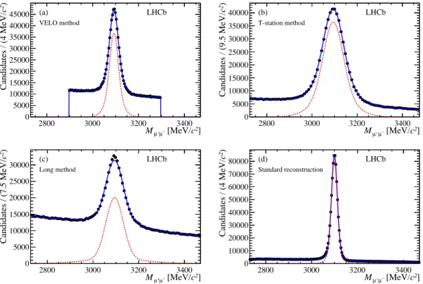
] 2 c [MeV/ − µ + µ M 2800 3000 3200 3400 ) 2c Candidates / (4 MeV/ 0 5000 10000 15000 20000 25000 30000 35000 40000 45000 (a) LHCb VELO method ] 2 c [MeV/ − µ + µ M 2800 3000 3200 3400 ) 2c Candidates / (9.5 MeV/ 0 5000 10000 15000 20000 25000 30000 35000 40000 (b) LHCb T-station method ] 2 c [MeV/ − µ + µ M 2800 3000 3200 3400 ) 2c Candidates / (7.5 MeV/ 0 5000 10000 15000 20000 25000 30000 (c)Long method LHCb ] 2 c [MeV/ − µ + µ M 2800 3000 3200 3400 ) 2 c Candidates / (4 MeV/ 0 10000 20000 30000 40000 50000 60000 70000 80000 (d) LHCb Standard reconstruction
Figure 3: Invariant mass distributions for reconstructed J/ψ candidates from the 2011 dataset. The solid line shows the fitted distribution for signal and background, the dotted line is the signal component. The subfigures are (a) the VELO method, (b) the T-station method, (c) the long method. For comparison of resolution and signal purity (d) shows the invariant mass distribution of J/ψ candidates obtained with the standard reconstruction at LHCb.
5.1
Mass resolution
To illustrate the mass resolutions that can be achieved, the dimuon invariant mass distributions from J/ψ candidates in the three methods are shown in Fig. 3 using the 2011 data sample. The difference in the visible ranges in Fig. 3(a) compared with the other distributions in Fig. 3 is a consequence of the different dimuon invariant mass cuts as listed in Table 2. The invariant mass distribution using two long tracks is shown in Fig. 3(d) for comparison. The signal peak is fitted with the sum of two Gaussian functions for this illustration. The effective mass resolution is about 24 MeV/c2 for the VELO method, 57 MeV/c2 for the T-station method and for the long method. This is to be compared to
the standard reconstruction with two long tracks that achieves a resolution of 16 MeV/c2.
6
Calculation of efficiency
The track reconstruction efficiency is calculated as the fraction of reconstructed J/ψ decays where the probe track can be matched to a long track. To estimate the number
of J/ψ decays, an unbinned extended maximum likelihood fit is performed to the mass distributions. For the VELO and T-station methods the mass distributions are described by a single Gaussian function for the signal and an exponential function for the combinatorial background. This model is preferred over the aforementioned sum of two Gaussian functions to improve the fit stability when measuring the dependence of the track reconstruction efficiency on kinematic variables and other event parameters. For the long method, a Crystal Ball function [29] is used for the signal, to take the tail on the left-hand side of the mass peak into account. Since the number of decays in the 2010 data is relatively low, in this case a simple sideband subtraction is applied for the VELO and T-station methods. All shape parameters were allowed to vary in the fit for the denominator of the efficiency; they were constrained to the found values for the numerator of the efficiency. This procedure was performed to stabilise the fit, as no difference in the shape of the numerator and denominator could be observed. It has been checked that the choice of the model for the mass distribution has a negligible effect on the efficiency determination.
The efficiencies obtained from the VELO and T-station methods are assumed to be uncorrelated, aside from effects due to dependencies on the track kinematics and the event multiplicity. The data sample is binned in kinematic variables and Ntrack to combine the
VELO and T-station efficiencies. The efficiencies obtained with the VELO and T-station methods can be multiplied in each bin to obtain the efficiency for finding long tracks. This combined efficiency can be compared with the efficiency found by the long method, giving two independent methods to probe the long track reconstruction efficiency.
There are, however, small differences between these two approaches. The long method measures the efficiency for tracks that pass through TT. In the combined method, only the VELO method requires this. Furthermore, both the VELO method and T-station method include the efficiency that, given that both the VELO and the T-station segment tracks are reconstructed, the corresponding long track is found. Therefore, in the combined efficiency, this so-called matching efficiency is counted twice. All these effects can lead to small differences in the measured long-track efficiency. For this reason, the ratio between the efficiencies in data and simulation is used to compare the methods, as these uncertainties are common for simulated and real decays and cancel when the ratio of efficiencies is formed.
On simulated events the track reconstruction efficiency is commonly defined as the fraction of simulated charged particles with sufficient hits in the VELO and T stations that can be associated to a track that shares at least 70% of the hits in each participating subdetector with this particle. For all methods, this so-called hit-based efficiency in simulation agrees within 1% with the efficiency measured with the tag-and-probe methods. Furthermore the matching efficiency was determined to be very close to 100%. The very small matching inefficiency does not affect the agreement between the hit-based efficiency and the tag-and-probe based efficiency in simulation. By taking the ratio between the efficiencies on data and simulation, these discrepancies are reduced to a negligible level.
Table 3: Track reconstruction efficiencies in % for the individual running periods using the long method for positive and negative muons and different magnetic field polarities (statistical uncertainties only).
Magnet up Magnet down
Data Positive Negative Positive Negative
2010 94.1 ± 1.3 96.0 ± 1.3 99.3+0.7−1.8 98.4+1.6−1.7 2011 97.0 ± 0.3 97.3 ± 0.3 97.2 ± 0.3 97.4 ± 0.3 2012 96.2 ± 0.2 96.2 ± 0.2 96.2 ± 0.2 96.3 ± 0.2
7
Efficiency dependencies
Using the momentum spectrum of the J/ψ decay products obtained with the VELO method from data as a benchmark, the average track reconstruction efficiency for long tracks is measured to be (95.4 ± 0.7)% for 2010 data, (97.78 ± 0.07)% for 2011 data and (96.99 ± 0.05)% for 2012 data. All results confirm the good performance of the LHCb tracking system. The uncertainties on these numbers are statistical only; they are binomial errors with additional terms to account for the statistical uncertainty on the number of background events. Systematic uncertainties are discussed in Sect. 8. The difference in the efficiencies between the three years is a consequence of changes in the track reconstruction and the higher centre-of-mass energy, leading to a higher track multiplicity and hence lower reconstruction efficiency for the 2012 running period. Dependencies on the polarity of the dipole magnet, the charge of the muons, and kinematic properties as well as the agreement with the simulation are investigated in further detail in the following subsections.
7.1
Comparison of magnetic field polarities
The track reconstruction efficiencies determined from the long method are split up into positively and negatively charged muons and into the two different magnetic field polarities (named up and down). The results are summarised in Table 3. They show compatible
numbers for magnetic field up and down and for positive and negative muons.
For data from 2011 and 2012 there is no difference between positive and negative muons or between the different magnet polarities. In 2010 data, a 2.3 σ difference between the different magnet polarities is observed for positive muons. No unambiguous source of the difference is found.
7.2
Dependencies of track reconstruction efficiency
The efficiency to reconstruct long tracks mainly depends on the particle kinematics and the number of charged particles in an event. As a parametrisation p, η and Ntrackare chosen, as
the track reconstruction efficiency shows the largest dependence on these three observables. The simulated events are weighted according to the Ntrack distribution observed in data.
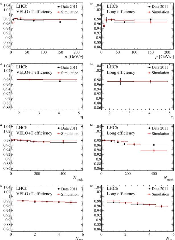
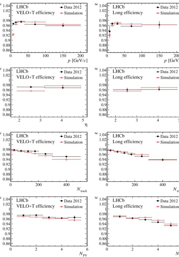
The track reconstruction efficiencies for the combination of the VELO and T-station methods and for the long method are shown for the different data-taking periods in Figs. 4–6 as a function of p, η, Ntrack, and as a function of the number of reconstructed
primary vertices, NPV. The efficiency coming from the combination of the VELO and
the T-station method is calculated by multiplying the individual efficiencies. Overall, a reasonable agreement is found between simulated and real data for all data-taking periods. As the agreement between the tag-and-probe based track reconstruction efficiency and the true track reconstruction efficiency (based on hit information) is within 1%, the results shown in Figs. 4–6 give an accurate description of the efficiency in simulation.
7.3
Efficiency ratios
The efficiency ratio is defined as the efficiency measured in data divided by the efficiency measured in simulation,
ratio = εdata εsim
. (1)
The efficiency dependence versus Ntrack and NPV is reasonably well described in the
simu-lation, see Figs. 4–6: When fitting a first-order polynomial to the efficiency distributions in simulation and real data, the slopes agree with each other within 2 standard deviations, except for the efficiency as a function of the number of tracks in the combination of the VELO and T-station method in 2012. It is therefore sufficient to weight the simulated events to establish agreement in Ntrack while the efficiency ratio is determined in bins of
p and η. The number of bins is chosen to keep the statistical uncertainty in each bin sufficiently small. For the final result, the weighted average of the combined and long method is taken in each bin of p and η.
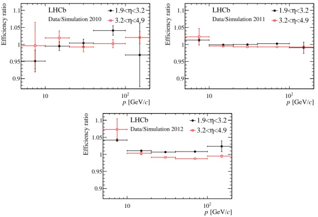
Figure 7 shows the efficiency ratio versus p for run I, weighted by the event track multiplicity observed in data; the data are split into two ranges of η. Overall a good agreement of the track finding efficiency is found between events in simulation and in data for all data taking periods and most momenta and pseudorapidity regions. The difference between the track finding efficiencies is generally smaller than 1% between events from simulation and data and no trend can be observed for the 2011 and 2012 dataset, with the number of events being too low to draw conclusions from the 2010 dataset. The agreement is worse for tracks with momentum below 10 GeV/c, which might point to a less accurate modelling of multiple scattering effects in the simulation.
The overall efficiency ratio and its uncertainty depend on the particle distribution of the data in terms of p and η. Using the momentum spectrum of the J/ψ decay products obtained with the VELO method from data, an average efficiency ratio is found of 0.994 ± 0.007 for 2010 data, 0.9983 ± 0.0009 for 2011 data and 1.0053 ± 0.0008 for 2012 data. The uncertainties represent the statistical uncertainties only. The ratio is close to one in all three cases as different features seen in the efficiency distributions in simulation and data average out when integrating over the full momentum spectrum or pseudorapidity range.
] c [GeV/ p 0 50 100 150 200 ε 0.86 0.88 0.9 0.92 0.94 0.96 0.98 1 1.02 1.04 Data 2010 Simulation LHCb VELO+T efficiency ] c [GeV/ p 0 50 100 150 200 ε 0.86 0.88 0.9 0.92 0.94 0.96 0.98 1 1.02 1.04 Data 2010 Simulation LHCb Long efficiency η 2 3 4 5 ε 0.86 0.88 0.9 0.92 0.94 0.96 0.98 1 1.02 1.04 Data 2010 Simulation LHCb VELO+T efficiency η 2 3 4 5 ε 0.86 0.88 0.9 0.92 0.94 0.96 0.98 1 1.02 1.04 Data 2010 Simulation LHCb Long efficiency track N 0 200 400 ε 0.86 0.88 0.9 0.92 0.94 0.96 0.98 1 1.02 1.04 Data 2010 Simulation LHCb VELO+T efficiency track N 0 200 400 ε 0.86 0.88 0.9 0.92 0.94 0.96 0.98 1 1.02 1.04 Data 2010 Simulation LHCb Long efficiency PV N 0 2 4 6 ε 0.86 0.88 0.9 0.92 0.94 0.96 0.98 1 1.02 1.04 Data 2010 Simulation LHCb VELO+T efficiency PV N 0 2 4 6 ε 0.86 0.88 0.9 0.92 0.94 0.96 0.98 1 1.02 1.04 Data 2010 Simulation LHCb Long efficiency
Figure 4: Track reconstruction efficiencies for the 2010 data and for weighted simulation. The left-hand column shows the results of the combined method while the right-hand column shows the results of the long method. The efficiency is shown as a function of p (first row), η (second row), Ntrack (third row), and NPV (fourth row). The error bars indicate the statistical uncertainties.
] c [GeV/ p 0 50 100 150 200 ε 0.86 0.88 0.9 0.92 0.94 0.96 0.98 1 1.02 1.04 Data 2011 Simulation LHCb VELO+T efficiency ] c [GeV/ p 0 50 100 150 200 ε 0.86 0.88 0.9 0.92 0.94 0.96 0.98 1 1.02 1.04 Data 2011 Simulation LHCb Long efficiency η 2 3 4 5 ε 0.86 0.88 0.9 0.92 0.94 0.96 0.98 1 1.02 1.04 Data 2011 Simulation LHCb VELO+T efficiency η 2 3 4 5 ε 0.86 0.88 0.9 0.92 0.94 0.96 0.98 1 1.02 1.04 Data 2011 Simulation LHCb Long efficiency track N 0 200 400 ε 0.86 0.88 0.9 0.92 0.94 0.96 0.98 1 1.02 1.04 Data 2011 Simulation LHCb VELO+T efficiency track N 0 200 400 ε 0.86 0.88 0.9 0.92 0.94 0.96 0.98 1 1.02 1.04 Data 2011 Simulation LHCb Long efficiency PV N 0 2 4 6 ε 0.86 0.88 0.9 0.92 0.94 0.96 0.98 1 1.02 1.04 Data 2011 Simulation LHCb VELO+T efficiency PV N 0 2 4 6 ε 0.86 0.88 0.9 0.92 0.94 0.96 0.98 1 1.02 1.04 Data 2011 Simulation LHCb Long efficiency
Figure 5: Track reconstruction efficiencies for the 2011 data and for weighted simulation. The left-hand column shows the results of the combined method while the right-hand column shows the results of the long method. The efficiency is shown as a function of p (first row), η (second row), Ntrack (third row), and NPV (fourth row). The error bars indicate the statistical uncertainties.
] c [GeV/ p 0 50 100 150 200 ε 0.86 0.88 0.9 0.92 0.94 0.96 0.98 1 1.02 1.04 Data 2012 Simulation LHCb VELO+T efficiency ] c [GeV/ p 0 50 100 150 200 ε 0.86 0.88 0.9 0.92 0.94 0.96 0.98 1 1.02 1.04 Data 2012 Simulation LHCb Long efficiency η 2 3 4 5 ε 0.86 0.88 0.9 0.92 0.94 0.96 0.98 1 1.02 1.04 Data 2012 Simulation LHCb VELO+T efficiency η 2 3 4 5 ε 0.86 0.88 0.9 0.92 0.94 0.96 0.98 1 1.02 1.04 Data 2012 Simulation LHCb Long efficiency track N 0 200 400 ε 0.86 0.88 0.9 0.92 0.94 0.96 0.98 1 1.02 1.04 Data 2012 Simulation LHCb VELO+T efficiency track N 0 200 400 ε 0.86 0.88 0.9 0.92 0.94 0.96 0.98 1 1.02 1.04 Data 2012 Simulation LHCb Long efficiency PV N 0 2 4 6 ε 0.86 0.88 0.9 0.92 0.94 0.96 0.98 1 1.02 1.04 Data 2012 Simulation LHCb VELO+T efficiency PV N 0 2 4 6 ε 0.86 0.88 0.9 0.92 0.94 0.96 0.98 1 1.02 1.04 Data 2012 Simulation LHCb Long efficiency
Figure 6: Track reconstruction efficiencies for the 2012 data and for weighted simulation. The left-hand column shows the results of the combined method while the right-hand column shows the results of the long method. The efficiency is shown as a function of p (first row), η (second row), Ntrack (third row), and NPV (fourth row). The error bars indicate the statistical uncertainties.
] c [GeV/ p 10 102 Efficiency ratio 0.9 0.95 1 1.05 1.1 1.9<η<3.2 <4.9 η 3.2< LHCb Data/Simulation 2010 ] c [GeV/ p 10 102 Efficiency ratio 0.9 0.95 1 1.05 1.1 1.9<η<3.2 <4.9 η 3.2< LHCb Data/Simulation 2011 ] c [GeV/ p 10 102 Efficiency ratio 0.9 0.95 1 1.05 1.1 1.9<η<3.2 <4.9 η 3.2< LHCb Data/Simulation 2012
Figure 7: Track reconstruction efficiency ratios as a function of p between data and simulation for (left) 2010 data, (right) 2011 data, and (bottom) 2012 data.
8
Systematic uncertainties
Small differences in the ratio of efficiencies are seen when reweighting the simulated samples in different parameters such as the number of primary vertices, or the number of hits or tracks in the different subdetectors. The largest of these differences is taken as a systematic uncertainty and amounts to 0.4%. No systematic uncertainty is assigned for the agreement of the track reconstruction efficiency determined by the tag-and-probe method and the hit-based method (which is on the order of 1%), as the differences cancel when forming the efficiency ratio. Accordingly, no systematic uncertainties are assigned for the fit model as these cancel when forming the fraction of reconstructed J/ψ decays where the probe can be matched to a long track. It has been checked that this is true for a range of fit models, the largest variation being 0.2%. Furthermore, no systematic uncertainty is assigned to the possible matching of a correctly reconstructed probe track to a fake long track, as the requirement for a large overlap in the subdetectors ensure that both reconstructed tracks are either real tracks or fake tracks, where the latter would not peak at the J/ψ mass. No systematic uncertainty is assigned for the fact that the VELO + T-station method and the long method show slightly different results in Figs. 4–6, as both methods probe different momentum spectra and any residual difference will cancel
when forming the ratio with simulation. No systematic uncertainty is assigned for the double-counting of the matching efficiency in the combined method, as this efficiency is very close to 100%, and any uncertainty would get further reduced when forming the ratio with simulation. No systematic uncertainty is assigned for the large difference for the VELO + T efficiency between simulation and data at low momenta in 2011 and 2012, as this is automatically taken into account when forming the ratio of efficiencies. Despite this difference, the integrated track reconstruction efficiencies between simulation and data are in agreement due to compensation of this effect for high momenta, where the efficiency is higher in simulation than in data.
9
Hadronic interactions
The methods presented in this paper are based on muons and require that they reach the muon stations. Thus, these methods are not sensitive to the effects from hadronic interactions and large-angle scatterings with the detector material. For hadrons, the largest effect is due to hadronic interactions. The cross section depends on the particle type, charge and the momentum. A simulation of B0 → J/ψ K∗0 decays (where K∗0→ K+π−) shows
that about 11% of the kaons (averaged over positive and negative kaons) and about 14% of the pions cannot be reconstructed due to hadronic interactions that occur before the last T station. This number depends primarily on the momentum of the particle. Due to the uncertainty on the material budget and consequently on the interaction with the detector material, the reconstruction efficiency obtained from simulation has an intrinsic uncertainty, which is not accounted for in the track reconstruction efficiencies measured with muons. When assuming that the total material budget in the simulation has an uncertainty of 10%, the systematic uncertainty due to hadronic interactions is between 1.1–1.4%. The 10% uncertainty is used as a conservative upper limit and is composed as follows: for the VELO a calculation in Ref. [4] shows an uncertainty on the material budget of 6%. No direct measurements exist for the T and TT stations. However, weight measurements for the Inner Tracker for the silicon sensors and the detector boxes give an accuracy of 2%, while an agreement of 5% is reached for the cables and the support structure [30, 31]. The Outer Tracker modules have been weighted and this measurement is precise to about 1% [32]. Furthermore, the sum of the weights of the individual components of a module adds up to the total weight of a module within the uncertainties. Taking into account that some level of detail is missing in the detector description in the simulation, an uncertainty of 5% is assumed for the outer tracker. Weight measurements for the sensor modules and the insulation material of TT have been performed. Given the detail of the detector description [33] an uncertainty of 5% on the material budget is well justified. The beam-pipe was implemented in the software following the design drawings, where a precision better than 10% for all pieces was confirmed following measurements after production. The solid radiator (aerogel) and the gas radiator (C4F10) contribute more than two-third
of the material budget for the RICH1 detector [34]. The amount of aerogel is known up to 2% and the differences between 2011 and 2012 are accounted for in the simulation. The
density of the C4F10 was monitored, with the RMS of the distribution being about 1%.
The other components of RICH1 have a smaller contribution to the interaction length. The overall uncertainty of 10% for the full material budget was then chosen to also take uncertainties on the Geant4 cross-sections and additional uncertainties, coming from simplified descriptions of the detector elements in the simulation, into account.
10
Conclusion
Track reconstruction efficiencies at LHCb have been measured using a tag-and-probe method with J/ψ → µ+µ− decays. The average efficiency is better than 95% in the
momentum region 5 GeV/c < p < 200 GeV/c and in the pseudorapidity region 2 < η < 5, which covers the phase space of LHCb. The uncertainty per track is below 0.5% for muons and below 1.5% for pions and kaons, where the larger uncertainty takes the uncertainty on hadronic interactions into account. All uncertainties have been added in quadrature. Furthermore, the ratio of the track reconstruction efficiency of muons in data and simulation is measured, where an uncertainty of 0.8 % for data collected in 2010 and an uncertainty of 0.4 % for data collected in 2011 and 2012 is achieved. The integrated efficiency ratios for all three years of data taking are compatible with unity. This result presents a significant improvement over the uncertainties determined with previous methods ranging from 3 to 4%.
Acknowledgements
We express our gratitude to our colleagues in the CERN accelerator departments for the excellent performance of the LHC. We thank the technical and administrative staff at the LHCb institutes. We acknowledge support from CERN and from the national agencies: CAPES, CNPq, FAPERJ, and FINEP (Brazil); NSFC (China); CNRS/IN2P3 (France); BMBF, DFG, HGF, and MPG (Germany); SFI (Ireland); INFN (Italy); FOM and NWO (The Netherlands); MNiSW and NCN (Poland); MEN/IFA (Romania); MinES and FANO (Russia); MinECo (Spain); SNSF and SER (Switzerland); NASU (Ukraine); STFC (United Kingdom); NSF (USA). The Tier1 computing centres are supported by IN2P3 (France), KIT and BMBF (Germany), INFN (Italy), NWO and SURF (The Netherlands), PIC (Spain), GridPP (United Kingdom). We are indebted to the communities behind the multiple open source software packages on which we depend. We are also thankful for the computing resources and the access to software R&D tools provided by Yandex LLC (Russia). Individual groups or members have received support from EPLANET, Marie Sk lodowska-Curie Actions, and ERC (European Union), Conseil g´en´eral de Haute-Savoie, Labex ENIGMASS, and OCEVU, R´egion Auvergne (France), RFBR (Russia), XuntaGal, and GENCAT (Spain), Royal Society and Royal Commission for the Exhibition of 1851 (United Kingdom).
References
[1] LHCb collaboration, R. Aaij et al., Measurement of σ(pp → bbX) at √s = 7 TeV in the forward region, Phys. Lett. B694 (2010) 209, arXiv:1009.2731.
[2] LHCb collaboration, R. Aaij et al., Production of J/ψ and Υ mesons in pp collisions at √s = 8 TeV, JHEP 06 (2013) 064, arXiv:1304.6977.
[3] LHCb collaboration, A. A. Alves Jr. et al., The LHCb detector at the LHC, JINST 3 (2008) S08005.
[4] R. Aaij et al., Performance of the LHCb Vertex Locator, JINST 9 (2014) 09007, arXiv:1405.7808.
[5] LHCb collaboration, LHCb reoptimized detector design and performance: Technical Design Report, CERN-LHCC-2003-030. LHCB-TDR-009.
[6] LHCb collaboration, LHCb inner tracker: Technical Design Report, CERN-LHCC-2002-029. LHCB-TDR-008.
[7] R. Arink et al., Performance of the LHCb Outer Tracker, JINST 9 (2014) P01002, arXiv:1311.3893.
[8] A. A. Alves Jr. et al., Performance of the LHCb muon system, JINST 8 (2013) P02022, arXiv:1211.1346.
[9] R. Aaij et al., The LHCb trigger and its performance in 2011, JINST 8 (2013) P04022, arXiv:1211.3055.
[10] T. Sj¨ostrand, S. Mrenna, and P. Skands, PYTHIA 6.4 physics and manual, JHEP 05 (2006) 026, arXiv:hep-ph/0603175.
[11] I. Belyaev et al., Handling of the generation of primary events in Gauss, the LHCb simulation framework, Nuclear Science Symposium Conference Record (NSS/MIC) IEEE (2010) 1155.
[12] D. J. Lange, The EvtGen particle decay simulation package, Nucl. Instrum. Meth. A462 (2001) 152.
[13] P. Golonka and Z. Was, PHOTOS Monte Carlo: a precision tool for QED corrections in Z and W decays, Eur. Phys. J. C45 (2006) 97, arXiv:hep-ph/0506026.
[14] Geant4 collaboration, J. Allison et al., Geant4 developments and applications, IEEE Trans. Nucl. Sci. 53 (2006) 270; Geant4 collaboration, S. Agostinelli et al., Geant4: a simulation toolkit, Nucl. Instrum. Meth. A506 (2003) 250.
[15] M. Clemencic et al., The LHCb simulation application, Gauss: design, evolution and experience, J. Phys. Conf. Ser. 331 (2011) 032023.
[16] D. Hutchcroft, VELO pattern recognition, CERN-LHCB-2007-013.
[17] O. Callot, FastVelo, a fast and efficient pattern recognition package for the Velo, LHCb-PUB-2011-001, CERN-LHCb-PUB-2011-001.
[18] O. Callot and S. Hansmann-Menzemer, The Forward Tracking, LHCb-2007-015, CERN-LHCb-2007-015.
[19] M. Needham and J. Van Tilburg, Performance of the track matching, LHCb-2007-020, CERN-LHCb-2007-020.
[20] M. Needham, Performance of the track matching, CERN-LHCB-2007-129.
[21] O. Callot and M. Schiller, PatSeeding: A standalone track reconstruction algorithm, CERN-LHCB-2008-042.
[22] O. Callot, Downstream pattern recognition, CERN-LHCB-2007-026.
[23] G. Manca, L. Mou, and B. Saitta, Studies of Efficiency of the LHCb Muon Detector Using Cosmic Rays, LHCb-PUB-2009-017.
[24] G. Passaleva, A recurrent neural network for track reconstruction in the LHCb Muon System, Nuclear Science Symposium Conference Record, 2008. NSS ’08. IEEE (2008) 867 .
[25] J. Albrecht, L. de Paula, A. P´erez-Calero Yzquierdo, and F. Teubert, Commissioning and Performance of the LHCb HLT1 muon trigger, LHCb-PUB-2011-006.
[26] V. V. Gligorov, A single track HLT1 trigger, LHCb-PUB-2011-003.
[27] J. Albrecht, V. Gligorov, G. Raven, and S. Tolk, Performance of the LHCb High Level Trigger in 2012, arXiv:1310.8544.
[28] F. Archilli et al., Performance of the muon identification at LHCb, JINST 8 (2013) P10020, arXiv:1306.0249.
[29] T. Skwarnicki, A study of the radiative cascade transitions between the Upsilon-prime and Upsilon resonances, PhD thesis, Institute of Nuclear Physics, Krakow, 1986, DESY-F31-86-02.
[30] V. Fave, Estimation of the material budget of the Inner Tracker, LHCb-2008-054, CERN-LHCb-2008-054.
[31] V. Fave, Survey of the Cables of the Inner Tracker, LHCb-2008-055, CERN-LHCb-2008-055.
[32] J. Nardulli and N. Tuning, A Study of the Material in an Outer Tracker Module, LHCb-2004-114, CERN-LHCb-2004-114.
[33] C. Salzmann and J. Van Tilburg, TT detector description and implementation of the survey measurements, LHCb-2008-061, CERN-LHCb-2008-061.
[34] LHCb RICH Collaboration, N. Brook et al., LHCb RICH1 Engineering Design Review Report, LHCb-2004-121. CERN-LHCb-2004-121.