HAL Id: hal-03013571
https://hal.uca.fr/hal-03013571
Preprint submitted on 20 Nov 2020
HAL is a multi-disciplinary open access archive for the deposit and dissemination of sci-entific research documents, whether they are pub-lished or not. The documents may come from teaching and research institutions in France or
L’archive ouverte pluridisciplinaire HAL, est destinée au dépôt et à la diffusion de documents scientifiques de niveau recherche, publiés ou non, émanant des établissements d’enseignement et de recherche français ou étrangers, des laboratoires
Dutch Disease in Africa: Evidence from a Panel of Nine
Oil-Exporting Countries
Edouard Mien
To cite this version:
Edouard Mien. External and Internal Real Exchange Rates and the Dutch Disease in Africa: Evidence from a Panel of Nine Oil-Exporting Countries. 2020. �hal-03013571�
C E N T R E D' ÉT U D E S E T D E R E C H E R C H E S S U R L E D E V E L O P P E M E N T I N T E R N A T I O N A L
SÉRIE ÉTUDES ET DOCUMENTS
External and Internal Real Exchange Rates and the Dutch Disease in
Africa: Evidence from a Panel of Nine Oil‐Exporting Countries
Edouard Mien
Études et Documents n°10
November 2020 To cite this document: Mien E. (2020) “External and Internal Real Exchange Rates and the Dutch Disease in Africa: Evidence from a Panel of Nine Oil‐Exporting Countries”, Études et Documents, n°10, CERDI. CERDI POLE TERTIAIRE 26 AVENUE LÉON BLUM F‐ 63000 CLERMONT FERRAND TEL. + 33 4 73 17 74 002 The author Edouard Mien PhD Student, School of Economics, University of Clermont Auvergne, CNRS, CERDI, F‐63000 Clermont‐Ferrand, France. Email address: edouard.mien@uca.fr Corresponding author: Edouard Mien
This work was supported by the LABEX IDGM+ (ANR‐10‐LABX‐14‐01) within the program “Investissements d’Avenir” operated by the French National Research Agency (ANR). Études et Documents are available online at: https://cerdi.uca.fr/etudes‐et‐documents/ Director of Publication: Grégoire Rota‐Graziosi Editor: Catherine Araujo‐Bonjean Publisher: Aurélie Goumy ISSN: 2114 ‐ 7957 Disclaimer:
Études et Documents is a working papers series. Working Papers are not refereed, they constitute
research in progress. Responsibility for the contents and opinions expressed in the working papers rests solely with the authors. Comments and suggestions are welcome and should be addressed to the authors.
Abstract
Despite a large number of empirical studies on Dutch disease in developing countries and the evidence that oil revenues tend to appreciate the real exchange rate, there remains little discussion about the definition of real exchange rates. This article intends to fill this gap by using four different proxies of the real exchange rate, differentiating the internal and the external real exchange rates for agricultural and manufacturing sectors. Using Pooled‐Mean‐ Group and Mean‐Group estimates on a panel of nine African net oil‐exporting countries, results show a clear appreciation of the RER generated by oil revenues except for the internal real exchange rate for manufacturing goods. This could imply that oil revenues more clearly affect agricultural compared to manufacturing competitiveness in these African countries. Keywords Dutch disease, Oil revenues, Pooled‐Mean‐Group estimator, Equilibrium real exchange rate, Africa JEL Codes C23, F31, 013, 024, 055 Acknowledgments I am thankful to Michael Goujon for his comments on the preliminary version of this paper. I also thank all FERDI staff members for all data and information provided, and particularly Camille Da Piedade for his help. I am finally thankful to all CERDI staff members for their helpful comments on my work.
1. Introduction
There is an important literature related to the role that natural resources, and especially oil, can play in explaining the absence of growth-producing structural transformations in several developing countries, and particularly in Africa (McMillan et al., 2014 ; Rodrik, 2016...). This question is even more prevalent today, due to the numerous discoveries in the 2010’s all around the continent of new reserves of oil (Niger and the Mozambique Channel at the beginning of the 2010 decade, Senegal in the mid-2010’s...) and gas (Egypt in the first half of the decade). One of the most common explanation for this phenomenon is the so-called Dutch disease (DD) effect, a widely known phenomenon that has been extensively discussed in the theoretical and empirical literature since the first models developed in the early 1980’s (Buiter and Purvis, 1980 ; Bruno and Sachs, 1982 ; Corden and Neary, 1982 ; van Wijnbergen, 1984....). This concept implies that natural resources tend to appreciate the real exchange rate (RER) through several channels which in return reduces the competitiveness of the non-resource tradable sector. Yet, despite the extensive literature on the subject, the question of the definition of RER has often been evacuated in empirical analyses. Indeed, one can broadly distinguish between two types of measures: the “internal” RER from the model of Corden and Neary (1982), defined as the ratio of price of non-tradable over tradable products, and the “external” RER, defined as the ratio of domestic over foreign prices. This distinction is important because those two indicators can be interpreted differently. The “internal” RER is a measure of the profitability differential between sectors, and hence explains structural transformations, whereas the “external” RER measures the external competitiveness of a country’s production, explaining declining export revenues in the non-resource sectors. Thus, both may not show the same patterns over time, especially when a boom occurs, while most empirical studies use only the external definition of the RER, even when they directly refer to the Corden-Neary model as the core theoretical model. There is then a clear and quite surprising gap between the importance of the discussion related to exchange rates in the early theoretical literature, and the empirical literature in which the external definition is predominant and in which the difference between both approaches is hardly ever discussed. This gap can be explained by three reasons. First, the external exchange rate has now become the canonical definition of the exchange rate in the economic literature. Second, even though their definitions differ, there is a mathematical relationship between the two RER (see section 3). Finally, while several institutions (World Bank, IMF, UNCTAD...) provide measures of the external RER, reliable data for internal RER are much more difficult to obtain. This remark is particularly true for developing countries, which have attracted most of the interest in the Dutch disease literature for the last two decades.
This paper intends to fill this gap by determining whether oil revenues have been associated in Africa with an appreciation of the external real exchange rate, with an appreciation of the internal real exchange rate, or both. Using a panel of nine African oil-exporting countries between 1995 and 2017, I investigate the long-run and short-run impacts of oil revenues on four different exchange rate indicators. These indicators correspond to the exchange rate computed for the main agricultural exports and for the main manufacturing exports for the internal and for the external exchange rates. The choice of using two indicators for each RER helps to strengthen the results and contributes to understand which export sector are the more likely to suffer from Dutch disease consequences. For this analysis, I apply the Pooled-Mean-Group estimator proposed by Pesaran et al. (1999) to the panel dataset and tests its robustness by using the Mean-Group estimators. I also use two different explanatory variables: oil revenues expressed in % of total GDP and the
international price of oil. Finally, I account for potential cross-sectional dependence by applying the Cross-Sectionally Augmented Pooled-Mean-Group estimator.
The panel data estimation reveals a clear and significant appreciation of the two external RER caused by oil revenues in the sample. Regarding internal measures of the RER, only the variable for agriculture clearly reveals the presence of a disease while the other variable provides mixed results, implying that oil revenues could have more agriculturalization” than “de-industrialization” effects in our panel.
The contribution of this article to the existing literature is threefold. First, it is the only attempt to investigate the effects of DD on four different RER to account for the difference between internal and external exchange rates and between manufactured and agricultural competitiveness. Second, it focuses on a panel of nine net oil-exporting African countries, while empirical analyses of Dutch disease in Africa usually explore country-case studies or on specific areas (such as Northern Africa or the CFA Franc Zone). Finally, this study exploits brand new indicators of RER. This last point is of special interest for the analysis of internal RER, due to the frequent lack of data in developing countries.
In a first step, I briefly review the theoretical and empirical literature relative to the impact of natural resource revenues on the RER and link the Dutch disease models with the literature relative to the determinants of long-run equilibrium exchange rate (section 2). Then, I detail the two definitions of the RER given in this article and discuss the relationship between them (section 3). Third, I describe the source of the data and justify the variables used in this paper (section 4). Then, I detail the econometric specification and the results and present several tests of robustness (section 5). The last section concludes and comments on the main limitations of the analysis (section 6).
2. A Short Review of Empirical and Theoretical Literature
2.1 The Dutch Disease Models
The term “Dutch disease” has been applied for the first time by the journal The Economist to describe the appreciation of the RER and the subsequent decline in competitiveness of the manufacturing sector in the Netherlands caused by gas exports during the 1960’s and 1970’s. Following this, a large theoretical literature has emerged in the early 1980’s to explain this phenomenon (Buiter and Purvis, 1980 ; Bruno and Sachs, 1982 ; Corden and Neary, 1982 ; van Wijnbergen, 1984...) with different assumptions, theoretical foundations and definitions.
Today, empirical studies almost always refer to the so-called model of Corden-Neary (Corden and Neary, 1982) and its extension (Corden, 1984) as the seminal theoretical model of Dutch disease. In that model, a boom in natural resources generates an exchange rate appreciation through two main channels: (i) by increasing public and private expenditures, it leads to a rise in the price of non-tradable goods while tradable goods prices are assumed exogenous (Spending effect), (ii) by attracting labor into the resource sector it puts pressure on wages in the two other sectors, leading to a rise in wages and hence in prices in the non-tradable sector while the wages in the tradable non-resource sectors are also exogenous (Resource-Movement Effect). In this model, the real
exchange rate is defined as the ratio of domestic tradable over domestic non-tradable goods (called the internal real exchange rate or IRER in the rest of this paper). Yet, other definitions of the RER have been proposed in several models. For instance, Buiter and Purvis (1980) define the RER as the ratio of domestic and foreign prices, following the currently most common definition of the exchange rate (called the external real exchange rate or ERER in the rest of this paper), but describe only the Spending effect. In this paper, I specifically target the link between natural resources revenues and the different real exchange rates to compare the predictions of these different models of Dutch disease. Another major point relative to these models is that they often assume the existence of a perfectly non-tradable and a perfectly non-resource tradable sector, while imperfect tradability could exist in some sectors. On the contrary, Benjamin et al. (1989) assume imperfect substitutability between foreign and domestic goods in the tradable sectors in the Cameroonian case, considering this assumption to be more relevant when studying developing countries. This implies that a disease could have different effects on the different tradable sectors, depending on their level of substitutability in international markets. This question will also be investigated here thanks to the use of different proxies of RER for agricultural and manufacturing products.
2.2 Equilibrium Exchange Rates and Fundamentals
We now turn to the theoretical and empirical studies relative to the determinants of the external real exchange rate because it has produced a much more abundant literature than the internal real exchange rate. Since the first Purchasing Power Parity approach coming back from Cassel (1916), there has been a large development of new approaches aiming at capturing the concept of “equilibrium exchange rate” and of short-run misalignment. Among them, the two most popular approaches are the Fundamental Equilibrium Exchange Rate (FEER) associated with Williamson (1994) and the Behavioural Equilibrium Exchange Rate proposed by Clark and MacDonald (1999) (for a more detailed description of all approaches see Egert et al., 2006). The FEER approach considers the equilibrium exchange rate as the exchange rate that simultaneously allows for external balance sustainability (exports equal imports) and for internal balance equilibrium (defined as the non-accelerating inflation rate of unemployment or NAIRU). On the contrary, the BEER approach focuses on a list of variables that are supposed to determine the long-run value of the real exchange rate. Since the paper from Clark and MacDonald, a large empirical literature has emerged, trying to estimate the main determinants of long-run real exchange rates. These fundamentals traditionally include GDP per capita or any other variable allowing to capture the Balassa-Samuelson effect, terms of trade, trade openness, public expenditures, investment, foreign capital inflows or net foreign assets... Consistent with the Dutch disease hypothesis, some studies also include causes for the DD in the fundamentals, such as international oil prices or resource revenues. This literature typically follows two steps. First, estimating the equilibrium exchange rate based on a set of fundamentals among the ones mentioned above. Then, computing the short-run misalignments defined as the difference between the equilibrium exchange rate estimated as the observed exchange rate.
In Africa, there has been an important literature relative to the understanding of exchange rate fundamentals. For instance, Roudet et al. (2007) estimate the impact of five fundamentals (terms of trade, government expenditures, openness, Balassa-Samuelson effect, and investment) on the exchange rate of WAEMU countries. For this, they first apply the Fully Modified Ordinary Least Squares (FMOLS) and the Pooled-Mean-Group (PMG) strategies to estimate the equilibrium RER
for the complete panel and find similar results with both methodologies. Then, they apply the Hodrick-Prescott filter to evaluate short-run misalignments and conclude to the presence of an overvaluation of the RER before the devaluation of the CFA Franc in 1994. Finally, they apply the Johansen maximum likelihood procedure and the ARDL approach to each country of the sample, allowing them to account for the heterogeneity in the panel. Similarly, Couharde et al. (2013) estimate the long-run relationship between the RER and a set of five fundamentals (terms of trade, Balassa-Samuelson, openness, public spending and NFA) in a panel of thirteen CFA area country members1) using Dynamic OLS (DOLS) estimation. They also use VECM methodology to capture
short-run dynamics for the variables. Nouira and Sekkat (2015) investigate the impact of five fundamentals (trade openness, net capital inflows, terms of trade, country debt service, government expenditures and Balassa-Samuelson effect) on the long-run equilibrium exchange rate using DOLS for a panel of 51 developing countries over 1980-2010. They also estimate short-run misalignments of this RER using the modified Hodrik-Prescott filter and find results that are overall consistent with the expectations.
2.3 Equilibrium Exchange Rates and the Dutch Disease
In line with the DD model, an important strand of the literature tries to estimate the impact of resource revenues on exchange rates, either considering resource revenues as a fundamental similar to trade openness or productivity per capita, or focusing on short-run variations caused by natural resources discoveries or international price variations. For example, by focusing on international oil price variations in a panel of 32 developing oil-producing countries and by implementing both a first-difference and a system-GMM methodology, Arezki and Ismail (2013) observe that oil prices are positively correlated with government spending which in return has an appreciation effect on the RER. This supports the evidence of a Spending effect in their panel of oil-exporting countries. Coudert et al. (2015) also investigate the impact of international commodity prices for a panel of 68 commodity exporters (including 26 developing, 37 intermediate and 5 advanced countries). Using Dynamic OLS, and accounting for cross-sectional dependence, they estimate the impact of three variables on long-run equilibrium exchange rates and on short-run ER variations: workers productivity (i.e. the Balassa-Samuelson effect), Net Foreign Assets, and what they call commodity Terms of Trade which aim to capture the variations of commodity prices. They finally conclude to an appreciation effect caused by commodities exports, with a much stronger coefficient in low income countries. In a country-case perspective, Essien and Akipan investigate the impact of a set of key fundamentals on the Nigerian equilibrium exchange rate (Essien and Akipan, 2016). They include the Balassa-Samuelson effect, the size of M2 in total economy, government expenditures, net foreign assets, trade openness and the international price of oil. In line with the DD, they conclude to a positive impact of oil prices on RER, with an average coefficient even higher than NFA, public expenditures and M2. It has also been argued in the empirical literature that Dutch disease could be driven by other channels than natural resources, such as international aid or migrant remittances. Regarding international aid, the seminal empirical investigation of Dutch disease in panel data comes from Rajan and Subramanian (2011). With a panel of 32 developing countries between 1980 and 2000, they estimate the impact of aid on several indicators, including a value for the excess appreciation of the RER based notably on the Balassa-Samuelson effect. Fielding and Gibson (2012) apply Vector Autoregressive (VAR) specifications to multiple
time-series for 36 African countries between 1970 and 2009. By including the logarithm of international aid commitment, the logarithm of real GDP, the logarithm of the real effective exchange rate and a dummy for the 1994 nominal devaluation for CFA countries, they observe that foreign aid can contribute to RER appreciation but with a large heterogeneity across countries. Similarly, Nketiah et al. (2019) estimate the long-run impact of remittances on the Ghanaian RER based on a Pooled OLS and including remittances, public expenditures, openness, capital inflows and terms of trade as fundamentals. Yet, their results are mixed, since the coefficient for remittances appears to be very low and mostly insignificant.
This article follows this empirical literature by assessing the impact of oil revenues on exchange rates in a panel of nine oil-exporting African countries. However, the aim is here only to determine the relationship between oil revenues and ER in oil-exporting countries. Then, the methodology implemented allows to evaluate short-run and long-run impacts of oil revenues variations on the RER but does not aim to estimate short-run misalignments from the equilibrium ER.
3. External and Internal Exchange Rates
The first question is the definition of the RER. Indeed, one can broadly define two different exchange rates. The “external” real exchange rate is the most popular interpretation of the exchange rate and corresponds to the ratio of domestic over foreign prices. On the contrary, some studies sometimes use what will be called here an “internal” exchange rate, defined as the ratio of domestic non-tradable over domestic tradables prices. It is noticeable that the seminal Corden-Neary model of Dutch disease never uses foreign prices but focuses only on the internal RER (Corden and Neary, 1982 ; Corden, 1984), contrary to Buiter and Purvis (1980) who prefer the external approach of the RER. Yet, surprisingly, most empirical studies of Dutch disease adopt the external RER, even when they directly refer to the model of Corden-Neary2.
Here, I follow Hinkle and Montiel (1999) and define the internal real exchange rate (IRER) and the external real bilateral exchange rate (ERER)3 as:
𝐼𝑅𝐸𝑅 𝑃𝑃;
; 1
With 𝑃; and 𝑃; the price indexes in non-tradable and tradable sectors respectively.
𝐸𝑅𝐸𝑅; 𝐸; .
𝑃
𝑃 2
With 𝐸; the nominal bilateral exchange rate between the two currencies, and 𝑃 and 𝑃 the price
2 One major exception is the study from Sala-i-Martin and Subramanian (2012) who exploit both internal and external exchange
rate indicators in their investigation of an oil curse in Nigeria.
3 For both the internal and the external exchange rates, there are always two different ways to define the ER and that depend on
which price index is the numerator and which is the denominator. Here, I define them such that an increase in the ratio always means an appreciation of the exchange rate.
indexes in countries i and j respectively. From equation 2, the external real effective exchange rate is given by:
𝐸𝑅𝐸𝐸𝑅 𝐸; .𝑃𝑃 3
With 𝛾 a weight given to each partner country j. Usually, this weight corresponds to the share of trade between country i and country j in total trade of country i. However, these weights can be measured differently. Since this study focuses on the external competitiveness of oil-exporting countries, I prefer another weight whose construction will be detailed in next section and capturing competitors rather than partners shares.
Let us now define 𝜆 as the share of tradables in total production of country j with 0 𝜆 1. It follows that 𝑃 𝑃; ∗ 𝑃;
Equation 3 then becomes:
𝐸𝑅𝐸𝐸𝑅 𝐸; . 𝑃; ∗ 𝑃; 𝑃; ∗ 𝑃; 𝐸; . 𝑃; 𝑃; ∗ 𝐸; . 𝑃; ∗ 𝑃; 𝑃; ∗ 𝑃; 𝐸; .𝑃𝑃; ; ∗ ⎝ ⎜ ⎛ 𝐸; . 𝑃; 𝑃; 𝑃; 𝑃; ⎠ ⎟ ⎞ We finally get: 𝐸𝑅𝐸𝐸𝑅 𝐸; .𝑃𝑃; ; ∗ 𝐸; . 𝐼𝑅𝐸𝑅 𝐼𝑅𝐸𝑅 4
Under the Law of One Price and assuming that the IRER of foreign countries are exogenous, a rise in the domestic IRER implies a similar rise in the EREER. However, if these assumptions are not met, the two RER can have different patterns over time. The rest of this paper therefore aims to estimate the impact of oil revenues on the internal and external RER given by equations 1 and 3.
4. Data
I use data from several sources (FERDI-OCD, World Economic Outlook, World development Indicators and the UNCTAD) for nine main African oil exporting countries between 1995 and 2017 to investigate the long-run relationship between the external and internal exchange rates and the set of fundamentals. The choice of this period corresponds to the availability of data for the
different measures of exchange rates. It also presents the advantage of including periods of booms and busts in oil production prices, and does not include the devaluation that occurred in the CFA Franc Zones countries in 1994 (which concerns four countries of the sample: Cameroon, the Republic of Congo, Equatorial Guinea and Gabon). I selected the countries among the main oil-producers in Africa according to the World Development Indicators (see table 5 in the Appendix). Since the empirical methodology applied here requires a variability in oil rent across time within each country, I included only countries which were net oil-exporters over the whole 1995-2017 period. Due to a lack of data availability and to the political instability that could have led to poor quality of data, I excluded Libya and Sudan from the sample, keeping nine net oil-exporting countries: Algeria, Angola, Cameroon, the Republic of Congo, Egypt, Equatorial Guinea, Gabon, Nigeria and Tunisia. Data sources are described in table 4. I detail in the following subsections the justification and definition of the variables used. Descriptive statistics and the matrix of correlation between all variables are displayed in the appendix.
4.1 The Dependent Variables
I use four different variables to capture the effects of oil revenues in net oil-exporting countries. The dependent variables all come from the Sustainable Competitiveness Observatory (OCD) of the Foundation for Studies and Research on International Development (FERDI) and are two internal and two external RER, computed for agricultural and manufacturing goods separately4.
Now I present the way these four proxies have been computed5. Regarding the internal real
exchange rates, both indicators are defined as:
𝐼𝑅𝐸𝑅 𝑃
𝑃 5
With P the consumer price index and 𝑃 ∑ 𝑠 with k the five main agricultural and five main manufactured products exported by the country and 𝑠 the share of each good k among these five exports. To avoid variations in the index that would not be caused by changes in prices but by changes in the share of each good among total exports, the weights 𝑠 attributed to each good k are constant over time and based on the average composition of exports over the period 2008-2012. The internal real exchange rates of the OCD are thus defined as the ratio of the price index over respectively agricultural exports prices and manufactured exports prices. This definition differs slightly from the IRER as defined in Corden and Neary (1982), but it is easily proved that they are linked with the following relationship6:
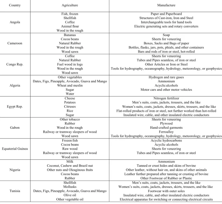
4 Agricultural products include food products either transformed or not (such as cereals, vegetables, fish, meat or dairy) as well as
primary goods produced for exports (such as coffee, rubber, tobacco or wood). Manufacturing products include transformed non-agricultural goods. For Angola and the republic of Congo which exports diamonds, the exchange rate variables have been computed by the author with the four other products using the reweighted average of the index of these products so that none of the exchange rate variables include oil or mineral products. For simplicity purpose, we will call them “agricultural” and “manufacturing” goods from now. The goods included in each exchange rate for each product is are detailed in the appendix (table 6).
5 All variables used are described in OCD (2017) and can be found at https:// competitivite.ferdi.fr/. The indexes are constructed by
the FERDI based on data from the Centre d’études prospectives et d’informations internationales (CEPII) and International
Financial Statistics (IFS). More details in the appendix.
𝐼𝑅𝐸𝑅 𝑃
𝑃 𝐼𝑅𝐸𝑅 6
It must be noted that the value in level for the exchange rates does not mean much in itself, the only condition required here is that changes in our proxy follow the same patterns as changes in the Corden-Neary internal real exchange rate. The choice of using average prices (estimated by the Consumer Price Index) instead of the price of non-tradables only is justified by the difficulty to differentiate perfectly non-tradable from other products. Indeed, while theoretical models tend to distinguish perfectly non-tradable from perfectly tradable goods, most goods are imperfectly tradable and differ in their level of tradability. In that case, it can be quite challenging to identify a representative basket of perfectly non-tradable goods or services. This issue is more easily dealt with for the basket of tradable goods since it is based on export prices, the most exported goods being here assumed to be representative of the main tradable goods.
We now move to the definitions of the external real effective exchange rates. Like the IRER, two indexes are constructed, both following the same equation:
𝐸𝑅𝐸𝐸𝑅 𝐸; .𝑃 ;
𝑃 ; 7
with 𝑃; the price of good k in country j and 𝐸; the bilateral nominal exchange rate between
countries i and j. Here, and contrary to the common definitions of the EREER used by the World Bank or the IMF, the weights attributed to each foreign country 𝛾 correspond to the share of each country j among total exports of good k in the world for the ten main exporting countries of good k. Therefore, the weights are not based on the partner shares of each country, but on competition between i and j. It is an important distinction from traditional empirical studies, which often use an index based on partner shares, especially for countries that are specialized in primary products and that do not export products to or import them from the countries that are specialized in the same production. Since the aim is to analyze the impact of resource revenues on external competitiveness, it seems more relevant to focus on competitors rather than trade partners. Due to the difficulty to aggregate price data from a large sample of countries, and the high imprecision that may result from the lack of data availability in many African countries, the index is restricted to the ten main exporters for each good k. Finally, the two indexes are computed as the weighted average for the five main agricultural and the five main manufactured goods separately, with 𝑠 the shares of each good k in exports of country i. Similarly to the IRER, the weights are constant over time and based on the shares calculated for the period 2008-2012. A major advantage of these variables is that, by focusing only on the five main agricultural and manufacturing exports, they do not include oil, contrary to traditional measures of the real effective exchange rate.
4.2 The Explanatory Variables
4.2.1 Oil Revenuesstraightforward variable is the share of resources (here oil) in total GDP or in total exports. This variable presents the advantage of directly capturing the impact of resource revenues on the economy. However, it also suffers from obvious endogeneity issues. First, for a given value of oil revenues, a poorer country will have a higher share of oil revenues in total GDP than a richer one. Reciprocally, one can assume that a more developed country will have more opportunities to develop a resource sector, or less incentives to do so, than a poor country. In both cases, the level of economic development affects the variable used for oil revenues. Another difficulty arising from the use of this variable is the fact that the shares of all sectors among total GDP adds up to 100%, i.e. a sudden drop or boom in one sector generates a symmetric rise or fall in the share of resource revenues in GDP even without any change in the resource sector, creating obvious reverse causality issues in empirical studies. However, this issue is particularly challenging when estimating the impact of resources on sectoral value-added, and not so much for exchange rate analysis.
The other most common strategy corresponds to the use of international prices (mainly oil prices such as the Brent or WTI crude oil price). The clear advantage of this variable relies on its supposed exogeneity7. However, this proxy is also subject to some key limitations. First, resource revenues
do not depend only on prices but also on other variables such as reserves discoveries or the political will to exploit natural resources. In that case, resource revenues can be weakly correlated with prices, making it more difficult to detect Dutch disease effects. Second, the exogeneity assumption requires that domestic resource production does not react to international price variations. Yet, a country or a firm can reduce its production when prices are low and increase it when they are high. In that case, oil revenues tend to overreact to oil prices movements.
A final strand of the literature relies on the timing of resource discoveries to estimate the impact of booms in production on the RER (for instance Arezki and Ismail, 2013). This methodology allows to implement different econometric strategies, such as difference-in-difference or synthetic control methods. I will not detail this literature here since, while it is helpful to estimate the impact of large booms, it is less useful when investigating the long-run relationships between resource revenues and exchange rates. This methodology also tends to require larger datasets than other strategies. Due to the main issues mentioned for the use of international oil prices, I choose here to use both oil revenues and international crude oil prices. For oil revenues, I use the traditional oil rent variable provided by the World Development Indicators and expressed in percent of total GDP. Regarding international oil prices, I exploit both the Brent and the West Texas Intermediate spot oil prices, which are the two main crude oil prices on international markets and the more likely to affect African oil prices to export.
4.2.2 Other Fundamentals
The control variables are the traditional fundamentals of the real effective exchange rate used in the literature on exchange rate misalignments, following the Behavioural Exchange Rate (BEER) approach. I select here four fundamentals among the most frequent in the literature.
The first fundamental is the degree of trade openness computed as the sum of total exports and
7 It is possible for some large oil exporters, such as Saudi Arabia, that the hypothesis of small economy is not verified. However,
total imports expressed in % of total GDP (from the UNCTAD). According to theoretical and empirical literature, this index is expected to be negatively associated with exchange rates. Indeed, from a theoretical point of view, higher trade barriers usually result in both lower trade openness and higher prices, hence implying a negative correlation between trade openness and real exchange rates (Égert et al., 2006). This argument is supported by the empirical studies for the external RER (Couharde et al., 2013 ; Diop et al., 2018...) Regarding our proxies for the internal RER, trade openness is expected to reduce domestic prices (the numerator) and thus the IRER.
I also include a proxy for the Balassa-Samuelson effect constructed by the FERDI-OCD as a ratio of oil GDP per capita against neighboring countries oil GDP per capita. The use of non-oil GDP is important because (i) it captures more precisely productivity gains (which is the goal of a Balassa-Samuelson index) than total GDP and (ii) it does not include oil resource booms (which would lead to underestimate the impact of our oil revenues variable). Theoretically, the expected sign of this proxy should be positive: an increase in total productivity is associated with an appreciation of the exchange rate. The empirical evidence in the literature is quite mixed but suggests overall to expect a positive sign for this variable. For instance, Coudert et al. (2015) find for a large panel of countries that productivity implies appreciation in low income countries but not in richer countries.
Then, I use a variable for Net Foreign Assets expressed in % GDP (from the UNCTAD). The theoretical literature suggests a positive relationship between NFA and exchange rates. However, empirical evidence remains mixed. Égert et al. (2006) argue that NFA may be negatively correlated with capital inflows in the medium-run but positively in the long-run (if foreign capital inflows are invested in the export sector, they will increase competitiveness and boost exports in the long-run). If capital inflows tend to generate an appreciation effect, one will observe a negative correlation between NFA and RER in the medium-run and a positive one in the long-run. In that case, the heterogeneity in results depends mainly on the number of periods in the sample (i.e. the size of T). In this case, the expected sign of NFA can also depend on the nature of foreign capital inflows and on the type of sector they are invested in, which depend themselves on the level of economic development. For instance, using a panel of countries with different levels of economic development, Coudert et al. (2015) observe a positive impact of NFA for developing countries (and to a lesser extent for advanced countries) but a negative coefficient for intermediate ones.
The final explanatory variable is the value of total investment (public and private) expressed in % of GDP. There is no consensus neither in the theoretical nor in the empirical literature on the expected sign for this variable. For instance, Diop et al. (2018) find a positive impact of investment on the RER in Senegal based on a Johansen and an ARDL model while Saxegaard (2007) finds a negative impact for this country. One could expect that, in the short-run, investment plays a role in appreciating the exchange rate (like consumption) by increasing domestic prices. However, in the long-run, investment can help firms to become more productive and reduce prices, generating depreciation effects. This effect however depends on the nature of investment (public or private, external or domestic...) and can differ across sectors.
Except for Net Foreign Assets and Oil Rent, all variables (including dependent and explanatory variables) are in logarithms. I do not include the terms of trade (which are also a common fundamental for the exchange rate in the empirical literature) since they could partly capture the
appreciation effect of the Dutch disease.
5. Methodology and Results
5.1 Integration and Co-Integration Tests
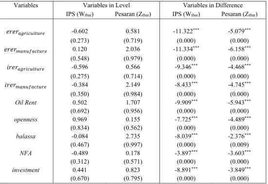
I begin by testing for the presence of unit-roots in the selected variables. For this, I apply the Panel-data unit-root test proposed by Im, Pesaran and Shin (2003) which has proved to provide consistent estimates even in small samples (Hurlin and Mignon, 2005). To account for potential cross-section dependence between countries in the variables of interest, I also use the test proposed by Pesaran (2003) which has been specifically designed to deal with this issue. Since the Brent and the WTI oil prices are repeated time-series, I use the simple time-series Augmented-Dickey-Fuller and Phillips-Perron unit-root tests for these two variables. Results are reported in tables 7 and 8 in the appendix. Both integration test results clearly indicate that all variables are I(1).
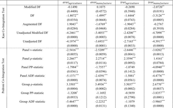
I test now for the presence of a co-integrating relationship among the variables. For this, I apply the test proposed by Kao (1999) and the test of Pedroni (2004). Indeed, the Kao co-integration test tends to have more power in small samples than other tests such as the original test proposed by Pedroni or the Larsson et al.’s (2001) co-integration tests (Gutierrez, 2003 ; Hurlin and Mignon, 2007). This test provides five statistics based on the Dickey-Fuller and Augmented Dickey-Fuller statistics, which are recognized to perform better in small-sample size panel than the Phillips-Perron based statistics (Davidson and MacKinnon, 2003). However, the Pedroni co-integration test has more power in sample with a fixed N and an increasing T and, compared to the previous tests, it also presents the advantage of overcoming the potential issue of more than one co-integration relationship between variables. This test provides seven different statistics, relying on different assumptions, and grouped into four Panel-Cointegration Statistics based on within-dimension and three Group-Mean Cointegration Statistics based on between-dimension. Results are reported in tables 9, 10 and 11. Overall, the results indicate to strongly reject the null hypothesis of absence of co-integration for the two external RER and for the internal RER for manufacture. Regarding the IRER for agricultural products, only four out of seven Pedroni statistics indicate to reject the null hypothesis when the main explanatory variable is oil rent and three for oil prices. Yet, all five statistics from Kao strongly suggest rejecting the null hypothesis of no co-integration, which seems more than enough to accept the hypothesis of co-integration among variables in the regressions.
5.2 Pooled-Mean-Group Estimation Results
Now, the aim is to estimate both the sign and the magnitude of the long-run relationships between each fundamental and the outcomes. The traditional empirical literature relative to the long-run determinants of real exchange rates in panel data has identified several econometric specifications to estimate such long-run relationships. These methods can be divided into two groups. In one side, pooling methods consist in using all data in the same regressions, and therefore require the assumption of homogeneity of effects across countries. On the contrary, “group-mean” specifications consist in (i) estimating the coefficients separately for each country and (ii) averaging them. These methods do not require the homogeneity assumption but have very low power due to the high number of coefficients to estimate. Therefore, I choose here to implement
the intermediate strategy of the Pooled Mean Group Estimators developed by Pesaran et al. (1999), which presents a higher power than averaging methods but requires weaker assumption than pooling ones. Indeed, the PMG relies on the assumption that long-run coefficients are homogeneous but not short-run coefficients. It consists in estimating the following equation:
Δ𝑦; 𝜙𝑦; 𝛽 𝑥; 𝜆; Δ𝑦; 𝛿; Δ𝑥; 𝜇 𝜖; 8
where 𝑦; is for each country i at time t computed as the logarithm of the external RER for agricultural and manufacturing goods, and of the internal RER for agricultural and manufacturing
goods (noted 𝑒𝑟𝑒𝑟 , 𝑒𝑟𝑒𝑟 , 𝑖𝑟𝑒𝑟 and 𝑖𝑟𝑒𝑟 )8. 𝑥
; is a set
of fundamentals that include our main explanatory variable and the four other control variables presented in section 4. The model also estimates the error-correction term, which indicates the speed of adjustment toward the long-run equilibrium and is expected to be between -1 and 0. Regressions are run first with Oil Rent and second with the two international oil prices as the main explanatory variable. The number of lags (p and q) is selected using the Bayesian Information Criteria, as recommended by Pesaran et al. (1999), with a maximum lag length of 1. Both the AIC and the BIC indicate to prefer an ARDL(111111) for each variable, except for 𝑖𝑟𝑒𝑟
with oil prices where an ARDL(111101) is preferred for the logarithm of the Brent oil price and an ARDL(111100) for the logarithm of the WTI oil price. The coefficients are then obtained through maximum likelihood estimation.
The PMG is preferred over the Mean-Group estimator for two reasons. First, due to the higher number of coefficients estimated in the MG specification, this strategy is very likely to provide imprecise and insignificant results, especially in a limited size sample like ours (207 observations). Second, according to Pesaran et al. (1999), PMG estimates also tend to be less sensitive to outliers than MG ones. The Mean-Group estimates are however also reported in the appendix (see tables 12 and 13). Pesaran et al. (1999) recommend comparing the long-run coefficients provided by MG and PMG specifications to ensure the validity of the second methodology. Since the Hausman test tests the null hypothesis that the long-run coefficients are not systematically different, and under the assumption that MG estimates are unbiased, it results in testing the hypothesis that the long-run PMG coefficients are unbiased. If the coefficients are observed to be significantly different from each other at 5% (i.e. if the p-value < 0.05), the PMG estimators might be biased and Mean-Group procedures are more likely to provide consistent estimates. Otherwise, we are inclined to prefer the PMG over the MG estimators. It must be underlined that this test is not a formal econometric proof that the PMG is or is not unbiased but only an evidence to support the idea that the PMG results can be interpreted, since we are primarily interested in the average long-run effect of oil revenues on the four exchange rates. It can also be noted that it tests the joint difference in coefficients and not the difference for each explanatory variable used separately. Results for the PMG estimates and for the Hausman tests are displayed in tables 1 and 2.
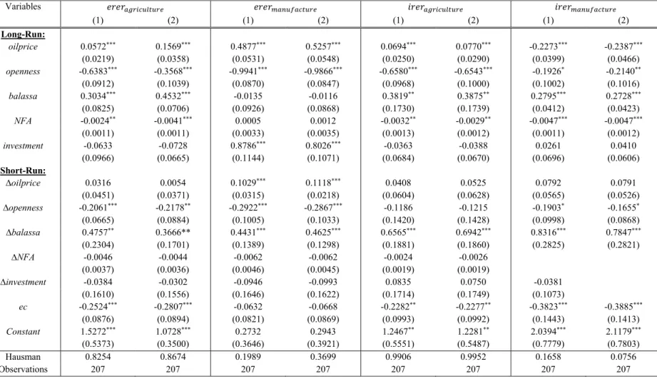
We can first observe a long-run positive and highly significant correlation between oil rent and all four exchange rates, supporting the Dutch disease hypothesis, both for the external and the internal
approaches. Regarding the IRER for manufacturing goods, the coefficient appears to be smaller than the three others, which can be attributed to a lower impact of oil rent on the manufacturing sector. However, due to the limits of the proxy used, one must remain careful about such interpretations, and more analyses are required. The results overall indicate that oil revenues are an important driver of RER fluctuations, even if the coefficient is lower than trade openness or the Balassa-Samuelson effect. Now, we turn to the impact of international oil prices. The results are very similar to the previous ones, with a positive and significant impact of the international Brent and the WTI oil prices on the two ERER and on the first IRER. Yet, the coefficient for manufacturing IRER, which was previously positive and significant at 5%, becomes here negative and significant at 1% in both cases. Two plausible explanations can be provided for this negative coefficient. First, one can assume that manufacture products are not perfectly tradable goods in our sample of countries, or that their degree of tradability is lower than the one of agricultural goods. Since the consumer price index used as the numerator in the construction of this variable includes tradable-goods, a low tradability of manufacturing goods can lead to a negative coefficient. In that case, the Dutch disease would be a concern for the agricultural sector rather than for the manufacturing one. Second, oil can be used as an input for the domestic production of manufacturing goods, meaning that an exogeneous price increase in international markets raises the production costs and the prices of these goods (even if the country is an exporter since oil-producing firms sell their production at the international market price even on domestic markets), counterbalancing the Dutch disease effects. However, the approximation used to construct the internal exchange rates is obviously imperfect and may also partly explain this surprising result. Regarding the other fundamentals, the coefficients are mainly as expected. The variable for trade openness is always negative and significant, in line with both theoretical and empirical literature, whereas the Balassa-Samuelson proxy is always positive except for the external exchange rate for manufacturing products, reinforcing the idea that agriculture and manufacture should be analyzed differently when estimating equilibrium exchange rates. Even if the coefficient for trade openness seems to be quite large when comparing it with other main determinants such as the Balassa-Samuelson effect or investment, its size remains reasonable. The only relatively surprising result is that Net Foreign Assets are indicated to generate depreciating effects while we were expecting an appreciation. Nevertheless, it is not in total contradiction with the literature since the evidence that NFA accumulation appreciates the ER is mixed in empirical analyses (see section 4). The variable for total investment is overall positive and strongly significant for the regressions based on oil rent. Finally, the error-correction term is as expected negative and most of the time significant.
The results for the Mean-Group estimators are displayed in tables 12 and 13 in the appendix, even when the Hausman test suggests accepting the PMG. As expected, the results are mostly insignificant even if the coefficients remain of the same sign that with the PMG. The few significant coefficients (𝑖𝑟𝑒𝑟 with oil rent, 𝑒𝑟𝑒𝑟 with WTI and 𝑖𝑟𝑒𝑟 with both Brent and WTI prices) also tend to support the evidence of a DD effect related to oil revenues.
Table 1: Pooled-Mean-Group Results for Oil Rent Variables 𝑒𝑟𝑒𝑟 𝑒𝑟𝑒𝑟 𝑖𝑟𝑒𝑟 𝑖𝑟𝑒𝑟 Long-Run: Oil Rent 0.0216*** 0.0190*** 0.0239*** 0.0053** (0.0029) (0.0023) (0.0031) (0.0025) openness -1.0164*** -0.8024*** -0.6813*** -0.6678*** (0.1142) (0.0964) (0.1064) (0.1316) balassa 0.5204*** 0.8065*** 0.9813*** 0.0524 (0.0885) (0.0770) (0.1116) (0.0647) NFA -0.0039*** -0.0023*** -0.0039*** -0.0096*** (0.0011) (0.0006) (0.0010) (0.0013) investment 0.3056*** 0.1675** 0.1199** 0.1918** (0.0977) (0.0749) (0.0589) (0.0782) Short-Run: ∆Oil Rent -0.0011 0.0004 -0.0050 0.0119 (0.0040) (0.0036) (0.0045) (0.0120) ∆openness -0.2054*** -0.2100*** -0.0323 -0.1155 (0.0679) (0.0736) (0.1804) (0.1114) ∆balassa 0.3880* 0.3579 0.4985*** 0.8202** (0.2279) (0.2237) (0.1825) (0.4111) ∆NFA -0.0044 -0.0038 -0.0032* -0.0048* (0.0034) (0.0033) (0.0016) (0.0027) ∆investment -0.1209 -0.1233 0.0076 -0.0082 (0.1888) (0.1752) (0.1893) (0.1198) ec -0.1491 -0.2254** -0.2351** -0.4702*** (0.0993) (0.1049) (0.1022) (0.1161) Constant 0.7961 0.8099** 0.5160** 3.2702*** (0.5401) (0.4133) (0.2509) (0.8124) Hausman 0.5462 0.9390 0.7995 Observations 207 207 207 207
Note: Hausman test reports the p-value for the Hausman test of PMG against MG. We prefer the Mean-Group over the Pooled-Mean-Group Estimator
if P < 0.05. In the last column, the Hausman statistic is negative, which could either indicate a strong evidence that we fail to reject the null hypothesis or that the model is misspecified. Variables in lower-case letters are expressed in logarithms, whereas Oil Rent and NFA are in % GDP. The number of lags is selected using the Bayesian Information Criterion. Standard errors are in parentheses. * Significant at 10%. ** Significant at 5%. ***Significant at 1%.
Table 2: Pooled-Mean-Group Results for Oil Prices
Note: Column (1) shows the results for the logarithm of the Brent oil price and column (2) for the logarithm of the WTI oil price. Hausman test reports the p-value for the Hausman test of PMG against MG.
We prefer the Mean-Group over the Pooled-Mean- Group Estimator if P < 0.05. Variables in lower-case letters are expressed in logarithms, whereas NFA is in % GDP. The number of lags is selected using the Bayesian Information Criterion. Standard errors are in parentheses. * Significant at 10%. ** Significant at 5%. ***Significant at 1%.
Variables 𝑒𝑟𝑒𝑟 𝑒𝑟𝑒𝑟 𝑖𝑟𝑒𝑟 𝑖𝑟𝑒𝑟 (1) (2) (1) (2) (1) (2) (1) (2) Long-Run: oilprice 0.0572*** 0.1569*** 0.4877*** 0.5257*** 0.0694*** 0.0770*** -0.2273*** -0.2387*** (0.0219) (0.0358) (0.0531) (0.0548) (0.0250) (0.0290) (0.0399) (0.0466) openness -0.6383*** -0.3568*** -0.9941*** -0.9866*** -0.6580*** -0.6543*** -0.1926* -0.2140** (0.0912) (0.1039) (0.0870) (0.0847) (0.0968) (0.1000) (0.1002) (0.1016) balassa 0.3034*** 0.4532*** -0.0135 -0.0116 0.3819** 0.3875** 0.2795*** 0.2728*** (0.0825) (0.0706) (0.0926) (0.0868) (0.1730) (0.1739) (0.0412) (0.0423) NFA -0.0024** -0.0041*** 0.0005 0.0012 -0.0032** -0.0029** -0.0047*** -0.0047*** (0.0011) (0.0011) (0.0033) (0.0035) (0.0013) (0.0012) (0.0011) (0.0012) investment -0.0633 -0.0728 0.8786*** 0.8026*** -0.0363 -0.0388 0.0261 0.0410 (0.0966) (0.0665) (0.1144) (0.1071) (0.0684) (0.0670) (0.0696) (0.0606) Short-Run: ∆oilprice 0.0316 0.0054 0.1029*** 0.1118*** 0.0408 0.0525 0.0792 0.0791 (0.0451) (0.0371) (0.0315) (0.0218) (0.0604) (0.0628) (0.0565) (0.0526) ∆openness -0.2061*** -0.2178** -0.2922*** -0.2867*** -0.1186 -0.1215 -0.1903* -0.1655* (0.0665) (0.0884) (0.1005) (0.1033) (0.1420) (0.1428) (0.0998) (0.0868) ∆balassa 0.4757** 0.3666** 0.4431*** 0.4625*** 0.6565*** 0.6942*** 0.8316*** 0.7847*** (0.2304) (0.1701) (0.1389) (0.1298) (0.1881) (0.1860) (0.2825) (0.2821) ∆NFA -0.0046 -0.0044 -0.0062 -0.0062 -0.0024 -0.0026 (0.0037) (0.0036) (0.0046) (0.0045) (0.0019) (0.0019) ∆investment -0.0384 -0.0302 -0.0946 -0.0993 0.0835 0.0750 -0.0381 (0.1610) (0.1556) (0.1646) (0.1622) (0.1714) (0.1749) (0.1073) ec -0.2524*** -0.2807*** -0.0632 -0.0668 -0.2282** -0.2277** -0.3823*** -0.3885*** (0.0876) (0.0894) (0.0821) (0.0869) (0.0993) (0.0992) (0.1443) (0.1413) Constant 1.5272*** 1.0728*** 0.2732 0.2943 1.2467** 1.2281** 2.0394*** 2.1179*** (0.5373) (0.3500) (0.3646) (0.3921) (0.5551) (0.5487) (0.7779) (0.7803) Hausman 0.8254 0.8674 0.1989 0.3699 0.9906 0.9952 0.1658 0.0756 Observations 207 207 207 207 207 207 207 207
5.3 Testing for Cross-Section Dependence
One common issue when dealing with panel data is the potential presence of cross-section dependence. This can occur when there is interdependence across countries such that a shock in each country can affect other countries, or when omitted shocks affect error terms in all countries. In that case, Pesaran et al. (1999) noted that the econometric model is likely to be misspecified. To test for the presence of cross-section dependence in the results, I implement the Breusch-Pagan Lagrange-Multiplier test (Breusch and Pagan, 1980). This test has indeed proved to be more efficient in panels with T larger than N than other tests, such as the CD test that is more efficient in panels with large N (Pesaran, 2015). Results are displayed in table 14 in the appendix and strongly suggest the presence of cross-section dependence in the model with Oil Rent as the main explanatory outcome. To deal with cross-section dependence, I follow the recommendation made by Pesaran et al. (1999) by implementing the Cross-Sectionally Augmented Pooled-Mean-Group (CPMG) approach used in several empirical papers such as Cavalcanti et al. (2012) or Grekou (2018). This strategy consists in including the cross-sectional average over all countries at time t for the variables of interest (written 𝑥 ∑ 𝑥; ) in the Pooled-Mean-Group estimation. The main drawback of this empirical strategy is that it increases the number of parameters to estimate. Due to the small size of our sample, it is unfortunately not possible to include all cross-section averages for all (dependent and explanatory) variables. It is noticeable that the four exchange rates and the proxy for the Balassa-Samuelson effect are defined as a base 100 index (equals to 100 in 2010 for all countries), hence the cross-section average (and the divergence for a given country from this average) does not make much sense here. I therefore restrict the regressions to include only the cross-section averages of three main explanatory variables, oil rent, trade openness and net foreign assets, which are the more likely to suffer from cross-section dependence because they are very likely to be affected by global shocks in international commodity prices. Since the international price of oil is a repeated time-series and is the same for each country, I cannot apply cross-sectionally augmented empirical strategies to this variable and restrict this procedure to the equation where oil rent is the main explanatory variable. Results are displayed in table 3.
The results tend to confirm the previous analyses, since the coefficients associated with oil rent are positive and strongly significant in the two first regressions and positive but less significant for the two internal exchange rates. All these results overall support the Dutch disease hypothesis, particularly for the agricultural sector since both external and internal exchange rate coefficients are significant, positive and of sizes that have economic sense.
Table 3: Cross-Sectionally Augmented Pooled-Mean-Group Results for Oil Rent Variables 𝑒𝑟𝑒𝑟 𝑒𝑟𝑒𝑟 𝑖𝑟𝑒𝑟 𝑖𝑟𝑒𝑟 Long-Run : 𝑂𝑖𝑙 𝑅𝑒𝑛𝑡 0.0035*** 0.0159*** 0.5155* 0.0064* (0.0013) (0.0029) (0.2639) (0.0037) 𝑜𝑝𝑒𝑛𝑛𝑒𝑠𝑠 -0.2293*** -0.9968*** -0.0735 -0.8729*** (0.0756) (0.0839) (0.7786) (0.1764) 𝑏𝑎𝑙𝑎𝑠𝑠𝑎 0.1107*** 0.6535*** -1.0615 -0.0785 (0.0191) (0.0617) (1.5531) (0.0854) 𝑁𝐹𝐴 -0.0022*** -0.0051*** -0.0804* -0.0095*** (0.0008) (0.0008) (0.0426) (0.0016) 𝑖𝑛𝑣𝑒𝑠𝑡𝑚𝑒𝑛𝑡 -0.0448 0.3484*** -1.5249 0.1087 (0.0353) (0.0766) (1.0146) (0.1143) 𝑂𝚤𝑙 𝑅𝑒𝑛𝑡 -0.0128*** 0.0075 -0.1452* -0.0380*** (0.0030) (0.0053) (0.0767) (0.0076) 𝑜𝑝𝑒𝑛𝑛𝑒𝑠𝑠 0.3753*** -0.1735 -7.6979* 1.6761*** (0.1010) (0.1866) (4.0508) (0.2528) 𝑁𝐹𝐴 0.0022 0.0061** -0.0287 0.0197*** (0.0014) (0.0025) (0.0348) (0.0037) Short-Run : Δ𝑂𝑖𝑙 𝑅𝑒𝑛𝑡 0.0024 0.0034 -0.0085 -0.0086 (0.0049) (0.0047) (0.0091) (0.0066) Δopenness -0.4730* -0.4212* -0.4195** -0.1771 (0.2574) (0.2309) (0.1866) (0.3235) Δ𝑏𝑎𝑙𝑎𝑠𝑠𝑎 0.0926 0.2639** 0.7486 0.2044 (0.1155) (0.1115) (0.5494) (0.2010) Δ𝑁𝐹𝐴 -0.0087 -0.0068 -0.0063* -0.0101 (0.0065) (0.0072) (0.0036) (0.0066) Δ𝑖𝑛𝑣𝑒𝑠𝑡𝑚𝑒𝑛𝑡 -0.0693 -0.1643 0.0946 0.0131 (0.1884) (0.1923) (0.0870) (0.1461) Δ𝑂𝚤𝑙 𝑅𝑒𝑛𝑡 -0.0019 -0.0024 0.0070 0.0061 (0.0043) (0.0038) (0.0096) (0.0047) Δ𝑜𝑝𝑒𝑛𝑛𝑒𝑠𝑠 0.7222 0.8461 0.1853 0.3128 (0.7286) (0.6193) (0.5699) (0.9217) Δ𝑁𝐹𝐴 0.0013 -0.0001 -0.0022 0.0018 (0.0021) (0.0030) (0.0064) (0.0051) ec -0.3774*** -0.2473** -0.0320 -0.4582*** (0.1249) (0.1096) (0.0246) (0.1221) Constant 1.4524*** 1.2612** 1.4625 0.8527*** (0.4794) (0.5679) (1.1328) (0.2250) Observations 207 207 207 207
Note: Variables in lower-case letters are expressed in logarithms, whereas Oil Rent and NFA are in % GDP. Standard errors are in parentheses.
6. Conclusion
Based on brand-new data, I investigate in this paper the long-run relationship between oil revenues and four different variables for the real exchange rate in nine main African net oil-exporting countries. The results clearly indicate that both the external interpretation of the Dutch disease (resource revenues weaken external competitiveness of other sectors and reduce non-resource exports) and the internal interpretation (resource revenues boost the development of non-tradable sectors at the expense of tradable ones and encourage structural transformations) are empirically confirmed in our panel of countries, supporting the seminal theoretical models of Dutch disease. From the external perspective, these findings imply that oil revenues tend to appreciate the exchange rate apart from its “classical” long-run fundamentals (such as trade openness or productivity per worker) and to make non-resource products less competitive on international markets. From an internal point of view, they generally confirm the model of Corden-Neary at least for agricultural products, implying that oil revenues can lead to “de-agriculturalization”. The evidence of a disease on both external and internal exchange rates for agricultural goods is of special interest for policy deciders by highlighting the importance for well-targeted public policies aiming at dealing with Dutch disease consequences not to neglect the agricultural sector. This is particularly relevant for African countries where agriculture often represents a higher share of the economy than manufacture, while empirical studies of Dutch disease focus more often on de-industrialization consequences. Another policy implication directly arises from the observation of differences between internal and external definitions of the RER. Indeed, the choice of the indicator selected to assess Dutch disease affects the results and the conclusions that can be drawn from these results. As mentioned earlier, there has been for the last decades a shift in empirical analyses toward the use of external definitions of exchange rates as the expense of internal ones. Yet, the two approaches differ in their interpretation and policymakers could benefit from using both types of indexes, depending on the issues they investigate.
However, these results should be carefully interpreted, due to major data limitations. In fact, the use of proxies for the internal exchange rates that do not perfectly correspond to the Corden-Neary definition of the RER, as well as the fact these proxies are based on a few products rather than on all exports by sectors, could have resulted in noise in the results. Therefore, more analyses are required to investigate the impact of natural resources on internal exchange rates, and to determine the differential impacts of Dutch disease effects on different tradable sectors. Finally, the empirical strategy implemented here does not allow to observe potential heterogeneity across countries. This is a major issue for external approaches in particular since all countries of the database do not share the same exchange rate and monetary targets (with four among the nine countries belonging to the common Central African CFA Franc Zone while the five other have adopted flexible nominal exchange rate policies). Further analyses relying on time-series could solve this issue and help to understand which countries in Africa are the most prone to Dutch disease.
7. Appendix
7.1 Mathematics
I investigate here the relationship between the OCD proxy for the two internal real exchange rates called 𝐼𝑅𝐸𝑅 and the internal exchange rate as defined in Corden and Neary (1982) and called 𝐼𝑅𝐸𝑅 . If we note α the share of the five main (agricultural and manufactured) exports in total domestic tradables such that 0 𝛼 1 and note 𝑃 the index of prices for the tradable goods that are not among the five main exports such that 𝑃 𝑃 ∗ 𝑃 9, then:
𝐼𝑅𝐸𝑅 𝑃 𝑃 𝑃 𝑃 . 𝑃 𝑃 𝑃 . 𝑃 𝑃 𝐼𝑅𝐸𝑅 𝑃 𝑃 𝑃 . 𝑃 𝑃 𝑃 . 𝑃 . 𝑃 . 𝑃 𝑃 . 𝑃 . 𝑃 . 𝑃 𝑃 𝑃 . 1 𝑃 . 𝑃 𝑃 . 𝑃 𝑃 𝑃 . 𝑃 𝑃 . 𝑃 𝑃 Thus: 𝐼𝑅𝐸𝑅 𝑃 𝑃 . 𝐼𝑅𝐸𝑅
Since 𝑃 𝑃 ∗ 𝑃 , we finally obtain:
𝐼𝑅𝐸𝑅 𝑃
𝑃 . 𝐼𝑅𝐸𝑅
Hence, there is a direct relationship between the internal real exchange rate and our proxy. Some main points must be noticed regarding this relationship:
Since λ < 1, the greater the share of traded goods in total domestic production (i.e. the greater λ), the greater the divergence between the internal real exchange rate as defined by Corden and Neary and its OCD proxy.
Due to possible changes in production structures, λ can change over time. Therefore, our proxy can change even when the internal exchange rate is constant (i.e. without changes in prices) if λ varies (i.e. with changes in the share of tradables among total production). Under the assumption that λ does not change, which is a plausible assumption in the short run, an increase in the IRER implies an increase in the proxy, but the relationship between them is not linear.
The higher the share of our five main exports among total tradables (i.e. the higher α), the lower the divergence between our proxy and the theoretical Corden-Neary IRER. The higher the divergence between 𝑃 and 𝑃 , the higher the divergence between our
proxy and the IRER of Corden-Neary. Since the exchange rates are always defined with a base 100 in a given year t, the comparisons in levels are not meaningful, but the variations in the exchange rates are. In our case, it means that a general fall in the price of all tradables (i.e. an increase in the external competitiveness), will not only directly affect the prices of all tradable goods 𝑝 ; but also the relative shares of H and X among T (some previously tradable but not exported goods will start being exported), and therefore that the difference between 𝑃 and 𝑃 decreases (making 𝐼𝑅𝐸𝑅 a better proxy for the Internal RER of Corden-Neary).
The impact of a variation in 𝑃 on 𝐼𝑅𝐸𝑅 is difficult to estimate: a rise in 𝑃 increases the ratio 𝑃 /𝑃 but is also likely to increase α (the non-ten best exports become less competitive hence the five best exports share in total exports rises) and reduce 1 − α.
7.2 Descriptive Statistics
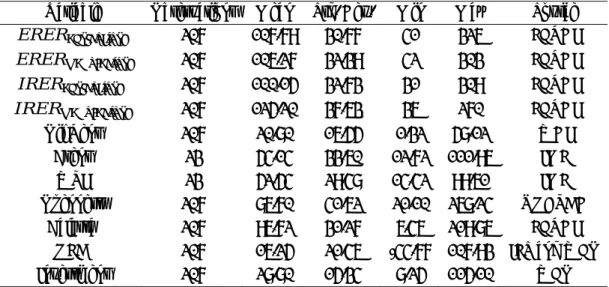
Table 4: Descriptive Statistics
Variable Observations Mean Std. Dev. Min Max Source
ERERagriculture 207 107.79 30.77 41 326 FERDI
ERERmanufacture 207 106.27 32.39 42 303 FERDI
IRERagriculture 207 100.15 32.73 31 309 FERDI
IRERmanufacture 207 125.20 37.63 36 270 FERDI
Oil Rent 207 20.80 16.55 1.32 58.12 WDI
Brent 23 54.14 33.60 12.72 111.96 IMF
WTI 23 52.54 29.48 14.42 99.61 IMF
Openness 207 86.70 41.62 21.10 268.24 UNCTAD
Balassa 207 96.72 31.27 6.46 219.86 FERDI
NFA 207 16.25 21.46 -44.77 107.93 IFS and WEO
Investment 207 28.80 15.34 8.25 115.10 WEO
“Oil Rent” is the share of oil revenues expressed in % GDP (World Development Indicators). Four observations are missing for Equatorial Guinea between 2001 and 2004. These data were reconstructed using country’s oil production (BEAC Central Bank) before 2001 and after 2005 and assuming similar trends.
“Brent” and “WTI” are respectively the Brent and WTI crude oil price per barrel (IMF Commodity Statistics Database). They are repeated time-series and are expressed in international US Dollars. “Trade Openness” is the sum of total exports and total imports expressed in % GDP (UNCTAD). Three observations are missing for Equatorial Guinea in 2017 and Gabon in 2016 and 2017. The data are reconstructed based on data for trade openness from the WDI and assuming similar trends.
“Balassa” is the ratio of domestic non-resource GDP per capita over foreign non-resource GDP per capita of the main partner countries (FERDI-OCD). It is in base 100 for the year 2010. Four observations are missing for Egypt between 1995 and 1998. They are reconstructed using FERDI-OCD data for the Balassa-Samuelson effect based on imports only and assuming similar trends.
“NFA” is the ratio of Net Foreign Assets held by the Central Bank (International Financial Statistics) over total GDP (World Economic Outlook). It is expressed in % GDP.
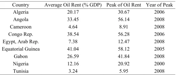
Table 5: Oil Rent by Country
Country Average Oil Rent (% GDP) Peak of Oil Rent Year of Peak
Algeria 20.17 30.67 2006
Angola 33.45 56.14 2008
Cameroon 4.64 8.91 2008
Congo Rep. 38.54 56.28 2006
Egypt, Arab Rep. 7.38 12.47 2008
Equatorial Guinea 41.04 58.12 2005
Gabon 26.59 41.84 2008
Nigeria 12.16 20.92 2000
Tunisia 3.24 5.95 2008
Note: Oil Rent is provided by the World Development Indicators. The mean and value of peak are based