HAL Id: hal-01966862
https://hal.archives-ouvertes.fr/hal-01966862
Submitted on 30 Dec 2018
HAL is a multi-disciplinary open access
archive for the deposit and dissemination of
sci-entific research documents, whether they are
pub-lished or not. The documents may come from
teaching and research institutions in France or
abroad, or from public or private research centers.
L’archive ouverte pluridisciplinaire HAL, est
destinée au dépôt et à la diffusion de documents
scientifiques de niveau recherche, publiés ou non,
émanant des établissements d’enseignement et de
recherche français ou étrangers, des laboratoires
publics ou privés.
Control via Protocol Composition
Mário Alvim, Konstantinos Chatzikokolakis, Yusuke Kawamoto, Catuscia
Palamidessi
To cite this version:
Mário Alvim, Konstantinos Chatzikokolakis, Yusuke Kawamoto, Catuscia Palamidessi. A
Game-Theoretic Approach to Information-Flow Control via Protocol Composition. Entropy, MDPI, 2018,
20 (5), pp.382. �10.3390/e20050382�. �hal-01966862�
Article
A Game-Theoretic Approach to Information-Flow
Control via Protocol Composition
Mário S. Alvim1,*ID, Konstantinos Chatzikokolakis2,3 ID, Yusuke Kawamoto4ID
and Catuscia Palamidessi2,5,*ID
1
Computer Science Department, Universidade Federal de Minas Gerais (UFMG), Belo Horizonte-MG 31270-110, Brazil
2 École Polytechnique, 91128 Palaiseau, France 3
Centre National de la Recherche Scientifique (CNRS), 91190 Gif-sur-Yvette, France; [email protected] 4
National Institute of Advanced Industrial Science and Technology (AIST), Tsukuba 305-8560, Japan; [email protected]
5
INRIA Saclay, 91120 Palaiseau, France
* Correspondence: [email protected] (M.S.A.); [email protected] (C.P.) Received: 24 March 2018; Accepted: 11 May 2018; Published: 17 May 2018
Abstract: In the inference attacks studied in Quantitative Information Flow (QIF), the attacker typically tries to interfere with the system in the attempt to increase its leakage of secret information. The defender, on the other hand, typically tries to decrease leakage by introducing some controlled noise. This noise introduction can be modeled as a type of protocol composition, i.e., a probabilistic choice among different protocols, and its effect on the amount of leakage depends heavily on whether or not this choice is visible to the attacker. In this work, we consider operators for modeling visible and hidden choice in protocol composition, and we study their algebraic properties. We then formalize the interplay between defender and attacker in a game-theoretic framework adapted to the specific issues of QIF, where the payoff is information leakage. We consider various kinds of leakage games, depending on whether players act simultaneously or sequentially, and on whether or not the choices of the defender are visible to the attacker. In the case of sequential games, the choice of the second player is generally a function of the choice of the first player, and his/her probabilistic choice can be either over the possible functions (mixed strategy) or it can be on the result of the function (behavioral strategy). We show that when the attacker moves first in a sequential game with a hidden choice, then behavioral strategies are more advantageous for the defender than mixed strategies. This contrasts with the standard game theory, where the two types of strategies are equivalent. Finally, we establish a hierarchy of these games in terms of their information leakage and provide methods for finding optimal strategies (at the points of equilibrium) for both attacker and defender in the various cases.
Keywords:information leakage; quantitative information flow; game theory; algebraic properties
1. Introduction
A fundamental problem in computer security is the leakage of sensitive information due to the correlation of secret values with observables, i.e., any information accessible to the attacker, such as, for instance, the system’s outputs or execution time. The typical defense consists of reducing this correlation, which can be done in, essentially, two ways. The first, applicable when the correspondence secret-observable is deterministic, consists of coarsening the equivalence classes of secrets that give rise to the same observables. This can be achieved with post-processing, i.e., sequentially composing the original system with a program that removes information from observables. For example, a typical
attack on encrypted web traffic consists of the analysis of the packets’ length, and a typical defense consists of padding extra bits so as to diminish the length variety [1].
The second kind of defense, on which we focus in this work, consists of adding controlled noise to the observables produced by the system. This can be usually seen as a composition of different protocols via probabilistic choice.
Example 1(Differential privacy). Consider a counting query f , namely a function that, applied to a dataset x, returns the number of individuals in x that satisfies a given property. A way to implement differential privacy [2] is to add geometrical noise to the result of f , so as to obtain a probability distribution P on integers of the form P(z) = c e∣z− f (x)∣, where c is a normalization factor. The resulting mechanism can be interpreted as a probabilistic choice on protocols of the form f(x), f (x) + 1, f (x) + 2, . . . , f (x) − 1, f (x) − 2, . . ., where the probability assigned to f(x) + n and to f (x) − n decreases exponentially with n.
Example 2(Dining cryptographers). Consider two agents running the dining cryptographers protocol [3], which consists of tossing a fair binary coin and then declaring the exclusive or ⊕ of their secret value x and the result of the coin. The protocol can be thought of as the fair probabilistic choice of two protocols, one consisting simply of declaring x and the other declaring x ⊕ 1.
Most of the work in the literature of Quantitative Information Flow (QIF) considers passive attacks, in which the attacker only observes the system. Notable exceptions are the works [4–6], which consider attackers who interact with and influence the system, possibly in an adaptive way, with the purpose of maximizing the leakage of information.
Example 3(CRIME attack). Compression Ratio Info-leak Made Easy (CRIME) [7] is a security exploit against secret web cookies over connections using the HTTPS and SPDY protocols and data compression. The idea is that the attacker can inject some content a into the communication of the secret x from the target site to the server. The server then compresses and encrypts the data, including both a and x, and sends back the result. By observing the length of the result, the attacker can then infer information about x. To mitigate the leakage, one possible defense would consist of transmitting, along with x, also an encryption method f selected randomly from a set F. Again, the resulting protocol can be seen as a composition, using probabilistic choice, of the protocols in the set F.
Example 4(Timing side-channels). Consider a password-checker, or any similar system in which the user authenticates himself/herself by entering a secret that is checked by the system. An adversary does not know the real secret, of course, but a timing side-channel could reveal the part (e.g., which bit) of the secret in which the adversary’s input fails. By repeating the process with different inputs, the adversary might be able to fully retrieve the secret. A possible counter measure is to make the side channel noisy, by randomizing the order in which the secret’s bits are checked against the user input. This example is studied in detail in Section7.
In all examples above, the main use of the probabilistic choice is to obfuscate the relation between secrets and observables, thus reducing their correlation; and hence, the information leakage. To achieve this goal, it is essential that the attacker never comes to know the result of the choice. In the CRIME example, however, if f and a are chosen independently, then (in general) it is still better to choose f probabilistically, even if the attacker will come to know, afterwards, the choice of f . In fact, this is true also for the attacker: his/her best strategies (in general) are to choose a according to some probability distribution. Indeed, suppose that F ={ f1, f2} are the defender’s choices and A = {a1, a2} are the
attacker’s and that f1(⋅, a1) leaks more than f1(⋅, a2), while f2(⋅, a1) leaks less than f2(⋅, a2). This is a
scenario like the matching pennies in game theory: if one player selects an action deterministically, the other player may exploit this choice and get an advantage. For each player, the optimal strategy is to play probabilistically, using a distribution that maximizes his/her own gain for all possible actions of the attacker. In zero-sum games, in which the gain of one player coincides with the loss of the
other, the optimal pair of distributions always exists, and it is called the saddle point. It also coincides with the Nash equilibrium, which is defined as the point at which neither of the two players gets any advantage in changing his/her strategy unilaterally.
Motivated by these examples, this paper investigates the two kinds of choice, visible and hidden (to the attacker), in a game-theoretic setting. Looking at them as language operators, we study their algebraic properties, which will help reason about their behavior in games. We consider zero-sum games, in which the gain (for the attacker) is represented by the leakage. While for the visible choice, it is appropriate to use the “classic” game-theoretic framework, for the hidden choice, we need to adopt the more general framework of the information leakage games proposed in [6]. This happens because, in contrast with standard game theory, in games with hidden choice, the payoff of a mixed strategy is a convex function of the distribution on the defender’s pure actions, rather than simply the expected value of their utilities. We will consider both simultaneous games, in which each player chooses independently, and sequential games, in which one player chooses his/her action first. We aim at comparing all these situations and at identifying the precise advantage of the hidden choice over the visible one.
To measure leakage, we use the well-known information-theoretic model. A central notion in this model is that of entropy, but here, we use its converse, vulnerability, which represents the magnitude of the threat. In order to derive results as general as possible, we adopt the very comprehensive notion of vulnerability as any convex and continuous function, as used in [4] and [8]. This notion has been shown [8] to be, in a precise sense, the most general information measure w.r.t. a set of fundamental information-theoretic axioms. Our results, hence, apply to all information measures that respect such fundamental principles, including the widely-adopted measures of Bayes vulnerability (also known as min-vulnerability, also known as (the converse of) Bayes risk) [9,10], Shannon entropy [11], guessing entropy [12] and g-vulnerability [13].
The main contributions of this paper are:
• We present a general framework for reasoning about information leakage in a game-theoretic setting, extending the notion of information leakage games proposed in [6] to both simultaneous and sequential games, with either a hidden or visible choice.
• We present a rigorous compositional way, using visible and hidden choice operators, for representing attacker’s and defender’s actions in information leakage games. In particular, we study the algebraic properties of visible and hidden choice on channels and compare the two kinds of choice with respect to the capability of reducing leakage, in the presence of an adaptive attacker.
• We provide a taxonomy of the various scenarios (simultaneous and sequential) showing when randomization is necessary, for either attacker or defender, to achieve optimality. Although it is well known in information flow that the defender’s best strategy is usually randomized, only recently has it been shown that when defender and attacker act simultaneously, the attacker’s optimal strategy also requires randomization [6].
• We compare the vulnerability of the leakage games for these various scenarios and establish a hierarchy of leakage games based on the order between the value of the leakage in the Nash equilibrium. Furthermore, we show that when the attacker moves first in a sequential game with hidden choice, the behavioral strategies (where the defender chooses his/her probabilistic distribution after he/she has seen the choice of the attacker) are more advantageous for the defender than the mixed strategies (where the defender chooses the probabilistic distribution over his/her possible functional dependency on the choice of the attacker). This contrast with the standard game theory, where the two types of strategies are equivalent. Another difference is that in our attacker-first sequential games, there may not exist Nash equilibria with deterministic strategies for the defender (although the defender has full visibility of the attacker’s moves). • We use our framework in a detailed case study of a password-checking protocol. A naive program,
because it reveals at each attempt (via a timing side-channel) the maximum correct prefix. On the other hand, if we continue checking until the end of the string (time padding), the program becomes very inefficient. We show that, by using probabilistic choice instead, we can obtain a good trade-off between security and efficiency.
Plan of the Paper
The remainder of the paper is organized as follows. In Section2, we review some basic notions of game theory and quantitative information flow. In Section3, we introduce our running example. In Section 4, we define the visible and hidden choice operators and demonstrate their algebraic properties. In Section 5, the core of the paper, we examine various scenarios for leakage games. In Section6, we compare the vulnerability of the various leakage games and establish a hierarchy among those games. In Section7, we show an application of our framework to a password checker. In Section8, we discuss related work, and finally, in Section9, we conclude.
A preliminary version of this paper appeared in [14]. One difference with respect to [14] is that in the present paper, we consider both behavioral and mixed strategies in the sequential games, while in [14], we only considered the latter. We also show that the two kinds of strategies are not equivalent in our context (Example10: the optimal strategy profile yields a different payoff depending on whether the defender adopts mixed strategies or behavioral ones). In light of this difference, we provide new results that concern behavioral strategies, and in particular:
• Theorem3, which concerns the defender’s behavioral strategies in the defender-first game with visible choice (Game II),
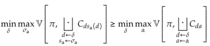
• the second half of Theorem6, which deals with the adversary’s behavioral strategies in the attacker-first game with hidden choice (Game VI).
Furthermore, in this paper, we define formally all concepts and provide all the proofs. In particular, we provide a precise formulation of the comparison among games with visible/hidden choices (Propositions4and5, Corollaries3–5) in Section6. Finally, in Section7, we provide a new result, expressed by Theorem7, regarding the optimal strategies for the defender in the presence of a uniform prior on passwords.
2. Preliminaries
In this section, we review some basic notions from game theory and quantitative information flow. We use the following notation: Given a set I, we denote byDI the set of all probability distributions over I. Given µ ∈DI, its support supp(µ)def= {i ∈ I ∶ µ(i) > 0} is the set of its elements with positive probability. We use i←µ to indicate that a value i∈I is sampled from a distribution µ on I. A set S ⊆ Rn is convex if ts0+ (1 − t)s1 ∈ S for all s0, s1 ∈ S and t ∈ [0, 1]. For such a set, a function
f ∶ S →Ris convex if f(ts0+ (1 − t)s1) ≤ t f (s0) + (1 − t) f (s1) for all s0, s1∈S, t ∈[0, 1], and concave
if − f is convex.
2.1. Basic Concepts from Game Theory 2.1.1. Two-Player Games
Two-player games are a model for reasoning about the behavior of two players. In a game, each player has at its disposal a set of actions that he/she can perform, and he/she obtains some gain or loss depending on the actions chosen by both players. Gains and losses are defined using a real-valued payoff function. Each player is assumed to be rational, i.e., his/her choice is driven by the attempt to maximize his/her own expected payoff. We also assume that the set of possible actions and the payoff functions of both players are common knowledge.
In this paper, we only consider finite games, in which the set of actions available to the players is finite, which are also zero-sum games, so the payoff of one player is the loss of the other. Next,
we introduce an important distinction between simultaneous and sequential games. In the following, we will call the two players defender and attacker.
2.1.2. Simultaneous Games
In a simultaneous game, each player chooses his/her action without knowing the action chosen by the other. The term “simultaneous” here does not mean that the players’ actions are chosen at the same time, but only that they are chosen independently. Formally, such a game is defined as a tuple (following the convention of security games, we set the first player to be the defender) (D, A, ud, ua), where D is a nonempty set of defender’s actions, A is a nonempty set of attacker’s
actions, ud ∶ D × A → R is the defender’s payoff function and ua ∶ D × A → Ris the attacker’s payoff function.
Each player may choose an action deterministically or probabilistically. A pure strategy of the defender (respectively attacker) is a deterministic choice of an action, i.e., an element d ∈ D (respectively a ∈ A). A pair(d, a) is called pure strategy profile, and ud(d, a), ua(d, a) represent the
defender’s and the attacker’s payoffs, respectively. A mixed strategy of the defender (respectively attacker) is a probabilistic choice of an action, defined as a probability distribution δ ∈DD (respectively
α ∈DA). A pair(δ, α) is called mixed strategy profile. The defender’s and the attacker’s expected payoff functions for mixed strategies are defined, respectively, as:
Ud(δ, α)def= E d←δ a←α ud(d, a) = ∑ d∈D a∈A δ(d)α(a)ud(d, a) and: Ua(δ, α) def = E d←δ a←α ua(d, a) = ∑ d∈D a∈A δ(d)α(a)ua(d, a).
A defender’s mixed strategy δ ∈ DD is the best response to an attacker’s mixed strategy
α ∈ DA if Ud(δ, α) = maxδ′∈DDUd(δ′, α). Symmetrically, α ∈DA is the best response to δ ∈DD if Ua(δ, α) = maxα′∈DAUd(δ, α′). A mixed-strategy Nash equilibrium is a profile (δ∗, α∗) such that δ∗is
the best response to α∗and vice versa. This means that in a Nash equilibrium, no unilateral deviation by any single player provides better payoff to that player. If δ∗and α∗are point distributions concentrated on some d∗ ∈D and a∗∈A, respectively, then(δ∗, α∗) is a pure-strategy Nash equilibrium and will be denoted by(d∗, a∗). While not all games have a pure strategy Nash equilibrium, every finite game has a mixed strategy Nash equilibrium.
2.1.3. Sequential Games
In a sequential game, players may take turns in choosing their actions. In this paper, we only consider the case in which each player moves only once, in such a way that one of the players (the leader) chooses his/her action first, and commits to it, before the other player (the follower) makes his/her choice. The follower may have total knowledge of the choice made by the leader, or only partial. We refer to the two scenarios by the terms perfect and imperfect information, respectively. Another distinction is the kind of randomization used by the players, namely whether the follower chooses probabilistically his/her action after he/she knows (partially or totally) the move of the leader, or whether he/she chooses at the beginning of the game a probabilistic distribution on (deterministic) strategies that depend on the (partial or total) knowledge of the move of the leader. In the first case, the strategies are called behavioral, in the second case mixed.
We now give the precise definitions assuming that the leader is the defender. The definitions for the case in which the leader is the attacker are analogous.
A defender-first sequential game with perfect information is a tuple(D, D → A, ud, ua) where
D, A, udand uaare defined as in simultaneous games: The choice of an action d ∈ D represents a
prior choice d of the defender, and for this reason, the pure strategies of the attacker are functions sa∶ D → A. As for the probabilistic strategies, those of the defender are defined as in simultaneous
games: namely, they are distributions δ ∈DD. On the other hand, the attacker’s probabilistic strategies can be defined in two different ways: In the behavioral case, an attacker’s probabilistic strategy is a function φa ∶ D → D(A). Namely, the attacker chooses a distribution on his/her actions after he/she sees the move of the defender. In the mixed case, an attacker’s probabilistic strategy is a probability distribution σa∈D(D → A). Namely, the attacker chooses a priori a distribution on pure strategies. The defender’s and the attacker’s expected payoff functions for mixed strategies are defined, respectively, as: Behavioral case: ⎧⎪⎪⎪⎪⎪⎨ ⎪⎪⎪⎪ ⎪⎩ Ud(δ, φa) def = E d←δa←φEa(d) ud(d, a) = ∑ d∈D δ(d) ∑ a∈A φa(d)(a) ud(d, a) Ua(δ, φa) def = E d←δa←φEa(d) ua(d, a) = ∑ d∈D δ(d) ∑ a∈A φa(d)(a) ua(d, a) Mixed case: ⎧⎪⎪⎪ ⎪⎪⎪⎪ ⎪⎨⎪ ⎪⎪⎪⎪ ⎪⎪⎪ ⎩ Ud(δ, σa) def = E d←δ sa←σa ud(d, sa(d)) = ∑ d∈D sa∶D → A δ(d)σa(sa)ud(d, sa(d)) Ua(δ, σa) def= E d←δ sa←σa ua(d, sa(d)) = ∑ d∈D sa∶D → A δ(d)σa(sa)ua(d, sa(d))
The case of imperfect information is typically formalized by assuming an indistinguishability (equivalence) relation over the actions chosen by the leader, representing a scenario in which the follower cannot distinguish between the actions belonging to the same equivalence class. The pure strategies of the followers, therefore, are functions from the set of the equivalence classes on the actions of the leader to his/her own actions. Formally, a defender-first sequential game with imperfect information is a tuple(D, Ka → A, ud, ua) where D, A, ud and uaare defined as in simultaneous games, and Kais a partition of D. The expected payoff functions are defined as before, except that now
the argument of φaand sais the equivalence class of d. Note that in the case in which all defender’s
actions are indistinguishable from each other in the eyes of the attacker (totally imperfect information), we have Ka={D}, and the expected payoff functions coincide with those of the simultaneous games.
In contrast, in the games in which all defender’s actions are distinguishable from the viewpoint of the attacker (perfect information), we have Ka={{d} ∣ d ∈ D}.
In the standard game theory, under the assumption of perfect recall (i.e., the players never forget what they have learned), behavioral and mixed strategies are equivalent, in the sense that for any behavioral strategy, there is a mixed strategy that yields the same payoff, and vice versa. This is true for both cases of perfect and imperfect information; see [15], Chapter 11.4. In our leakage games, however, this equivalence does not hold anymore, as will be shown in Sections5and6.
2.1.4. Zero-Sum Games and the Minimax Theorem
A game(D, A, ud, ua) is zero-sum if for any d ∈ D and any a ∈ A, the defender’s loss is equivalent
to the attacker’s gain, i.e., ud(d, a) = −ua(d, a). For brevity, in zero-sum games, we denote by u the
attacker’s payoff function uaand by U the attacker’s expected payoff Ua(Conventionally in game
theory, the payoff u is set to be that of the first player, but we prefer to look at the payoff from the point of view of the attacker to be in line with the definition of payoff as vulnerability.). Consequently, the goal of the defender is to minimize U, and the goal of the attacker is to maximize it.
In simultaneous zero-sum games, the Nash equilibrium corresponds to the solution of the minimax problem (or equivalently, the maximin problem), namely the strategy profile(δ∗, α∗) such that U(δ∗, α∗) = min
δmaxαU(δ, α). The von Neumann’s minimax theorem, in fact, ensures that such a solution (which always exists) is stable.
Theorem 1 (von Neumann’s minimax theorem). Let X ⊂ Rm and Y ⊂ Rn be compact convex sets, and U ∶ X × Y →Rbe a continuous function such that U(x, y) is a convex function in x ∈ X and a concave function in y ∈ Y. Then:
min
x∈X maxy∈Y U(x, y) = maxy∈Y minx∈XU(x, y).
A related property is that, under the conditions of Theorem1, there exists a saddle point(x∗, y∗) s.t., for all x ∈ X and y ∈ Y: U(x∗, y) ≤ U(x∗, y∗) ≤ U(x, y∗).
The solution of the minimax problem can be obtained by using convex optimization techniques. In the case U(x, y) is affine in x and in y, we can also use linear optimization.
In the case D and A contain two elements each, there is a closed form for the solution. Let D ={d0, d1} and A = {a0, a1}, respectively. Let uij be the payoff of the defender on di, aj. Then,
the Nash equilibrium(δ∗, α∗) is given by: δ∗(d0) = u u11−u10
00−u01−u10+u11 α
∗(a
0) = u u11−u01
00−u01−u10+u11 (1)
if these values are in[0, 1]. Note that, since there are only two elements, the strategy δ∗is completely specified by its value in d0and analogously for α∗.
2.2. Quantitative Information Flow
Finally, we briefly review the standard framework of quantitative information flow, which is concerned with measuring the amount of information leakage in a (computational) system.
2.2.1. Secrets and Vulnerability
A secret is some piece of sensitive information the defender wants to protect, such as a user’s password, social security number or current location. The attacker usually only has some partial knowledge about the value of a secret, represented as a probability distribution on secrets called a prior. We denote by X the set of possible secrets, and we typically use π to denote a prior belonging to the setDX of probability distributions over X .
The vulnerability of a secret is a measure of the payoff that it represents for the attacker. In this paper, we consider a very general notion of vulnerability, following [8], and we define a vulnerability Vto be any continuous and convex function of typeDX → R. It has been shown in [8] that these functions coincide with the set of g-vulnerabilities, and are, in a precise sense, the most general information measures w.r.t. a set of fundamental information-theoretic axioms (more precisely, if posterior vulnerability is defined as the expectation of the vulnerability of posterior distributions, the measure respects the fundamental information-theoretic properties of data-processing inequality (i.e., that post-processing can never increase information, but only destroy it) and of non-negativity of leakage (i.e., that by observing the output of a channel, an actor cannot, on average, lose information) if, and only if, vulnerability is convex). This notion, hence, subsumes all information measures that respect such fundamental principles, including the widely-adopted measures of Bayes vulnerability (also known as min-vulnerability, also known as (the converse of) Bayes risk) [9,10], Shannon entropy [11], guessing entropy [12] and g-vulnerability [13].
2.2.2. Channels, Posterior Vulnerability and Leakage
Computational systems can be modeled as information theoretic channels. A channel C ∶ X × Y → Ris a function in which X is a set of input values, Y is a set of output values and C(x, y) represents the conditional probability of the channel producing output y ∈ Y when input x ∈ X is provided. Every channel C satisfies 0 ≤ C(x, y) ≤ 1 for all x ∈ X and y ∈ Y, and ∑y∈YC(x, y) = 1 for
all x ∈ X .
A distribution π ∈DX and a channel C with inputs X and outputs Y induce a joint distribution p(x, y) = π(x)C(x, y) on X × Y, producing joint random variables X, Y with marginal probabilities
p(x) = ∑yp(x, y) and p(y) = ∑xp(x, y), and conditional probabilities p(x∣y) =p(x,y)/p(y)if p(y) ≠ 0.
For a given y (s.t. p(y) ≠ 0), the conditional probabilities p(x∣y) for each x ∈ X form the posterior distribution pX∣y.
A channel C in which X is a set of secret values and Y is a set of observable values produced by a system can be used to model computations on secrets. Assuming the attacker has prior knowledge π about the secret value, knows how a channel C works and can observe the channel’s outputs, the effect of the channel is to update the attacker’s knowledge from π to a collection of posteriors pX∣y, each occurring with probability p(y).
Given a vulnerabilityV, a prior π and a channel C, the posterior vulnerabilityV[π, C] is the vulnerability of the secret after the attacker has observed the output of the channel C. Formally: V[π, C]def= ∑y∈Yp(y)V[pX∣y].
Consider, for instance, the example of the password-checker with a timing side-channel from the Introduction (Example4, also discussed in detail in Section7). Here, the set of secrets X consists of all possible passwords (say, all strings of n bits), and a natural vulnerability function is Bayes-vulnerability, given byV(π) = maxx∈X π(x). This function expresses the adversary’s probability of guessing correctly the password in one try; assuming that the passwords are chosen uniformly, i.e., π is uniform, any guess would be correct with probability 2−n, givingV(π) = 2−n. Now, imagine that the timing side-channel reveals that the adversary’s input failed on the first bit. The adversary now knows the first bit of the password (say 0); hence, the posterior pX∣yassigns probability zero to all passwords with first bit one and probability 2−(n−1)to all passwords with first bit zero. This happens for all possible posteriors, giving posterior vulnerabilityV[π, C] = 2−(n−1)(two-times greater than the priorV).
It is known from the literature [8] that the posterior vulnerability is a convex function of π. Namely, for any channel C, any family of distributions{πi} and any set of convex coefficients {ci},
we have: V[∑ i ciπi, C] ≤ ∑ i ciV[πi, C]
The (information) leakage of channel C under prior π is a comparison between the vulnerability of the secret before the system was run (called prior vulnerability) and the posterior vulnerability of the secret. Leakage reflects how much the observation of the system’s outputs increases the attacker’s information about the secret. It can be defined either additively (V[π, C] −V[π]) or multiplicatively (V[π,C]/V[π]). In the password-checker example, the additive leakage is 2−(n−1)− 2−n=2−n, and the
multiplicative leakage is2−(n−1)/2−n=2.
3. An Illustrative Example
We introduce an example that will serve as a running example throughout the paper. Although admittedly contrived, this example is simple and yet produces different leakage measures for all different combinations of visible/hidden choice and simultaneous/sequential games, thus providing a way to compare all different scenarios in which we are interested.
Consider that a binary secret must be processed by a program. As usual, a defender wants to protect the secret value, whereas an attacker wants to infer it by observing the system’s output. Assume the defender can choose which among two alternative versions of the program to run. Both programs take the secret value x as high input and a binary low input a whose value is chosen by the attacker. They both return the output in a low variable y (we adopt the usual convention in QIF of referring to secret variables, inputs and outputs in programs as high and to their observable counterparts as low). Program 0 returns the binary product of x and a, whereas Program 1 flips a coin with bias
a/3(i.e., a coin that returns heads with probability a/3) and returns x if the result is heads and the
Program 0 High Input:x ∈{0, 1} Low Input:a ∈{0, 1} Output:y ∈{0, 1} y = x ⋅ a return y Program 1 High Input:x ∈{0, 1} Low Input:a ∈{0, 1} Output:y ∈{0, 1} c ← flip coin with biasa/3
if c = heads{y = x} else{y = x} return y
Figure 1.Alternative programs for the running example.
The combined choices of the defender’s and of the attacker’s determine how the system behaves. Let D = {0, 1} represent the set of the defender’s choices, i.e., the index of the program to use, and A ={0, 1} represent the set of the attacker’s choices, i.e., the value of the low input a. We shall refer to the elements of D and A as actions. For each possible combination of actions d ∈ D and a ∈ A, we can construct a channel Cdamodeling how the resulting system behaves. Each channel Cdais a
function of type X × Y →R, where X ={0, 1} is the set of possible high input values for the system and Y ={0, 1} is the set of possible output values from the system. Intuitively, each channel provides the probability that the system (which was fixed by the defender) produces output y ∈ Y given that the high input is x ∈ X (and that the low input was fixed by the attacker). The four possible channels are depicted in Table1.
Table 1.The four channels Cdafor d, a ∈{0, 1} for the running example.
C00 y = 0 y = 1 x = 0 1 0 x = 1 1 0 C01 y = 0 y = 1 x = 0 1 0 x = 1 0 1 C10 y = 0 y = 1 x = 0 0 1 x = 1 1 0 C11 y = 0 y = 1 x = 0 1/3 2/3 x = 1 2/3 1/3
Note that channel C00does not leak any information about the input x (i.e., it is non-interferent),
whereas channels C01and C10completely reveal x. Channel C11is an intermediate case: it leaks some
information about x, but not all.
We want to investigate how the defender’s and the attacker’s choices influence the leakage of the system. For that, we can just consider the (simpler) notion of posterior vulnerability, since in order to make the comparison fair, we need to assume that the prior is always the same in the various scenarios, and this implies that the leakage is in a one-to-one correspondence with the posterior vulnerability (this happens for both additive and multiplicative leakage).
For this example, assume we are interested in Bayes vulnerability [9,10], defined as V(π) = maxxπ(x) for every π ∈DX . Assume for simplicity that the prior is the uniform prior πu.
In this case, we know from [16] that the posterior Bayes vulnerability of a channel is the sum of the greatest elements of each column, divided by the total number of inputs. Table2provides the Bayes vulnerabilityVda
def
= V[πu, Cda] of each channel considered above.
Table 2.Bayes vulnerability of each channel Cdafor the running example.
V a = 0 a = 1
d = 0 1/2 1 d = 1 1 2/3
Naturally, the attacker aims at maximizing the vulnerability of the system, while the defender tries to minimize it. The resulting vulnerability will depend on various factors, in particular on whether the two players make their choice simultaneously (i.e., without knowing the choice of the opponent) or sequentially. Clearly, if the choice of a player who moves first is known by an opponent who moves second, the opponent will be at an advantage. In the above example, for instance, if the defender knows the choice a of the attacker, the most convenient choice for him/her is to set d = a, and the vulnerability will be at most2/3. The other way around, if the attacker knows the choice d of the defender, the most convenient choice for him/her is to set a ≠ d. The vulnerability in this case will be one.
Things become more complicated when players make choices simultaneously. None of the pure choices of d and a are the best for the corresponding player, because the vulnerability of the system depends also on the (unknown) choice of the other player. Yet, there is a strategy leading to the best possible situation for both players (the Nash equilibrium), but it is mixed (i.e., probabilistic), in that the players randomize their choices according to some precise distribution.
Another factor that affects vulnerability is whether or not the defender’s choice is known to the attacker at the moment in which he/she observes the output of the channel. Obviously, this corresponds to whether or not the attacker knows what channel he/she is observing. Both cases are plausible: naturally, the defender has all the interest in keeping his/her choice (and hence, the channel used) secret, since then, the attack will be less effective (i.e., leakage will be smaller). On the other hand, the attacker may be able to identify the channel used anyway, for instance because the two programs have different running times. We will call these two cases hidden and visible choice, respectively.
It is possible to model players’ strategies, as well as hidden and visible choices, as operations on channels. This means that we can look at the whole system as if it were a single channel, which will turn out to be useful for some proofs of our technical results. The next section is dedicated to the definition of these operators. We will calculate the exact values for our example in Section5.
4. Choice Operators for Protocol Composition
In this section, we define the operators of visible and hidden choice for protocol composition. These operators are formally defined on the channel matrices of the protocols, and since channels are a particular kind of matrix, we use these matrix operations to define the operations of visible and hidden choice among channels and to prove important properties of these channel operations.
4.1. Matrices and Their Basic Operators
Given two sets X and Y, a matrix is a total function of type X × Y → R. Two matrices M1 ∶ X1 × Y1 → R and M2 ∶ X2× Y2 → Rare said to be compatible if X1 = X2. If it is also the case that Y1 =Y2, we say that the matrices have the same type. The scalar multiplication r⋅M
between a scalar r and a matrix M is defined as usual, and so is the summation(∑i∈IMi) (x, y) =
Mi1(x, y) + . . . + Min(x, y) of a family {Mi}i∈Iof matrices all of a same type.
Given a family {Mi}i∈I of compatible matrices s.t. each Mi has type X × Yi → R, their concatenation ◇i∈I is the matrix having all columns of every matrix in the family, in such a way that
every column is tagged with the matrix from which it came. Formally,(◇i∈IMi) (x, (y, j)) = Mj(x, y),
if y ∈ Yj, and the resulting matrix has type X × (⨆i∈IYi) →R. (We use⨆i∈IYi=Yi1⊔ Yi2⊔ . . . ⊔ Yin
to denote the disjoint union{(y, i) ∣ y ∈ Yi, i ∈ I} of the sets Yi1, Yi2, . . ., Yin.) When the family{Mi}
has only two elements we may use the binary version ⋄ of the concatenation operator. The following depicts the concatenation of two matrices M1and M2in tabular form.
M1 y1 y2 x1 1 2 x2 3 4 ⋄ M2 y1 y2 y3 x1 5 6 7 x2 8 9 10 = M1⋄ M2 (y1, 1) (y2, 1) (y1, 2) (y2, 2) (y3, 2) x1 1 2 5 6 7 x2 3 4 8 9 10
4.2. Channels and Their Hidden and Visible Choice Operators
A channel is a stochastic matrix, i.e., all elements are non-negative, and all rows sum up to one. Here, we will define two operators specific for channels. In the following, for any real value 0 ≤ p ≤ 1, we denote by p the value 1 − p.
4.2.1. Hidden Choice
The first operator models a hidden probabilistic choice among channels. Consider a family{Ci}i∈I
of channels of the same type. Let µ ∈DI be a probability distribution on the elements of the index set I. Consider an input x is fed to one of the channels in{Ci}i∈I, where the channel is randomly
picked according to µ. More precisely, an index i ∈ I is sampled with probability µ(i), then the input x is fed to channel Ci, and the output y produced by the channel is then made visible, but not the
index i of the channel that was used. Note that we consider hidden choice only among channels of the same type: if the sets of outputs were not identical, the produced output might implicitly reveal which channel was used.
Formally, given a family{Ci}i∈Iof channels s.t. each Cihas same type X × Y →R, the hidden choice operator⨊i←µis defined as⨊i←µCi =∑i∈Iµ(i) Ci.
Proposition 1(Type of hidden choice). Given a family{Ci}i∈I of channels of type X × Y → R, and a distribution µ on I, the hidden choice⨊i←µCiis a channel of type X × Y →R.
See AppendixAfor the proof.
In the particular case in which the family{Ci} has only two elements Ci1and Ci2, the distribution
µon indexes is completely determined by a real value 0 ≤ p ≤ 1 s.t. µ(i1) = p and µ(i2) = p. In this
case, we may use the binary version p
⊕
of the hidden choice operator: Ci1 p⊕
Ci2 = p Ci1+p Ci2.The example below depicts the hidden choice between channels C1and C2, with probability p=1/3.
C1 y1 y2 x1 1/2 1/2 x2 1/3 2/3 1/3
⊕
C2 y1 y2 x1 1/3 2/3 x2 1/2 1/2 = C11/3⊕
C2 y1 y2 x1 7/18 11/18 x2 4/9 5/9 4.2.2. Visible ChoiceThe second operator models a visible probabilistic choice among channels. Consider a family {Ci}i∈Iof compatible channels. Let µ ∈DI be a probability distribution on the elements of the index
set I. Consider an input x is fed to one of the channels in{Ci}i∈I, where the channel is randomly
picked according to µ. More precisely, an index i ∈ I is sampled with probability µ(i), then the input x is fed to channel Ci, and the output y produced by the channel is then made visible, along with the
index i of the channel that was used. Note that visible choice makes sense only between compatible channels, but it is not required that the output set of each channel be the same.
Formally, given{Ci}i∈Iof compatible channels s.t. each Cihas type X × Yi→R, and a distribution µon I, the visible choice operator&i←µis defined as&i←µCi= ◇i∈I µ(i) Ci.
Proposition 2(Type of visible choice). Given a family{Ci}i∈I of compatible channels s.t. each Ci has
type X × Yi → R and a distribution µ on I, the result of the visible choice&i←µCi is a channel of type X × (⨆i∈IYi) →R.
See AppendixAfor the proof.
In the particular case that the family{Ci} has only two elements Ci1 and Ci2, the distribution µ
case, we may use the binary version p
H
of the visible choice operator: Ci1 pH
Ci2 = p Ci1⋄ p Ci2.The following depicts the visible choice between channels C1and C3, with probability p=1/3.
C1 y1 y2 x1 1/2 1/2 x2 1/3 2/3 1/3
H
C3 y1 y3 x1 1/3 2/3 x2 1/2 1/2 = C11/3H
C3 (y1, 1) (y2, 1) (y1, 3) (y3, 3) x1 1/6 1/6 2/9 4/9 x2 1/9 2/9 1/3 1/34.3. Properties of Hidden and Visible Choice Operators
We now prove algebraic properties of channel operators. These properties will be useful when we model a (more complex) protocol as the composition of smaller channels via hidden or visible choice.
Whereas the properties of hidden choice hold generally with equality, those of visible choice are subtler. For instance, visible choice is not idempotent, since in general Cp
H
C ≠ C (in fact, if C hastype X × Y →R, C p
H
C has type X × (Y ⊔ Y) →R). However, idempotency and other properties involving visible choice hold if we replace the notion of equality with the more relaxed notion of “equivalence” between channels. Intuitively, two channels are equivalent if they have the same inputspace and yield the same value of vulnerability for every prior and every vulnerability function. Definition 1 (Equivalence of channels). Two compatible channels C1 and C2 with domain X are
equivalent, denoted by C1 ≈ C2, if for every prior π ∈ DX and every posterior vulnerabilityV, we have V[π, C1] = V[π, C2].
Two equivalent channels are indistinguishable from the point of view of information leakage, and in most cases, we can just identify them. Indeed, nowadays, there is a tendency to use abstract channels [8,17], which capture exactly the important behavior with respect to any form of leakage. In this paper, however, we cannot use abstract channels because the hidden choice operator needs a concrete representation in order to be defined unambiguously.
The first properties we prove regard idempotency of operators, which can be used do simplify the representation of some protocols.
Proposition 3(Idempotency). Given a family{Ci}i∈Iof channels s.t. Ci=C for all i ∈ I, and a distribution
µ on I, then: (a)⨊i←µCi =C; and (b)&i←µCi ≈C.
See AppendixAfor the proof.
The following properties regard the reorganization of operators, and they will be essential in some technical results in which we invert the order in which hidden and visible choice are applied in a protocol.
Proposition 4(“Reorganization of operators”). Given a family{Cij}i∈I,j∈J of channels indexed by sets I
and J , a distribution µ on I and a distribution η on J : (a) ⨊i←µ⨊j←ηCij=⨊i←µ
j←η
Cij, if all Ci’s have the same type;
(b) &i←µ&j←ηCij≈&i←µ j←η
Cij, if all Ci’s are compatible; and
(c) ⨊i←µ&j←ηCij≈&j←η⨊i←µCij, if, for each i, all Cij’s have the same type X × Yj →R. See AppendixAfor the proof.
Finally, analogous properties of the binary operators are shown in AppendixB. 4.4. Properties of Vulnerability w.r.t. Channel Operators
We now derive some relevant properties of vulnerability w.r.t. our channel operators, which will be later used to obtain the Nash equilibria in information leakage games with different choice operations.
The first result states that posterior vulnerability is convex w.r.t. hidden choice (this result was already presented in [6]) and linear w.r.t. to visible choice.
Theorem 2(Convexity/linearity of posterior vulnerability w.r.t. choices). Let{Ci}i∈I be a family of
channels and µ be a distribution on I. Then, for every distribution π on X and every vulnerabilityV: 1. posterior vulnerability is convex w.r.t. to hidden choice:V[π, ⨊i←µCi] ≤ ∑i∈Iµ(i)V[π, Ci] if all Ci’s
have the same type.
2. posterior vulnerability is linear w.r.t. to visible choice:V[π, &i←µCi] = ∑i∈Iµ(i)V[π, Ci] if all Ci’s
are compatible.
Proof. 1. Let us call X × Y →Rthe type of each channel Ciin the family{Ci}. Then:
V⎡⎢⎢⎢⎢⎢⎢⎢ ⎣ π,⨊ i←µ Ci⎤⎥⎥⎥⎥⎥⎥⎥ ⎦ =V[π, ∑
iµ(i)Ci] (by the definition of hidden choice)
= ∑
y∈Y
p(y) ⋅V[
π(⋅) ∑iµ(i)Ci(⋅, y)
p(y) ] (by the definition of posteriorV) = ∑ y∈Y p(y) ⋅V[∑ i µ(i)π(⋅)Ci(⋅, y) p(y) ] ≤ ∑ y∈Y p(y) ⋅ ∑ i
µ(i)V[π(⋅)Cp(y)i(⋅, y)] (by the convexity ofV) =∑ i µ(i) ∑ y∈Y p(y)V[ π(⋅)Ci(⋅, y) p(y) ] =∑ i µ(i)V[π, Ci]
where p(y) = ∑x∈X π(x) ∑iµ(i)Ci(x, y).
2. Let us call X × Yi→Rthe type of each channel Ciin the family{Ci}. Then: V⎡⎢⎢⎢⎢⎢⎢⎢
⎣π,i←µ'
Ci⎤⎥⎥⎥⎥⎥⎥⎥
⎦
=V[π, ◇iµ(i)Ci] (by the definition of visible choice) = ∑
y∈Y
p(y) ⋅V[π(⋅) ◇ip(y)µ(i)Ci(⋅, y)] (by the definition of posteriorV) = ∑ y∈Y p(y) ⋅V[◇iµ(i)π(⋅)Ci(⋅, y) p(y) ] = ∑ y∈Y p(y) ⋅ ∑ i
µ(i)V[π(⋅)Cp(y)i(⋅, y)] (see (*) below) =∑ i µ(i) ∑ y∈Y p(y)V[π(⋅)Cp(y)i(⋅, y)] =∑ i µ(i)V[π, Ci]
where p(y) = ∑x∈X π(x) ∑iµ(i)Ci(x, y), and step (*) holds because in the vulnerability of a
weight in the concatenation; hence, it is possible to break the vulnerability of a concatenated matrix as the weighted sum of the vulnerabilities of its sub-matrices.
The next result is concerned with posterior vulnerability under the composition of channels using both operators.
Corollary 1(Convex-linear payoff function). Let{Cij}i∈I,j∈J be a family of channels, all with domain X
and with the same type, and let π ∈DX , andVbe any vulnerability. Define U ∶DI ×DJ →Ras follows: U(µ, η)def
= V[π, ⨊i←µ&j←η Cij]. Then, U is convex on µ and linear on η. Proof. To see that U(µ, η) is convex on µ, note that:
U(µ, η) =V⎡⎢⎢⎢⎢⎢⎢⎢ ⎣ π,⨊ i←µ ' j←η Cij⎤⎥⎥⎥⎥⎥⎥⎥ ⎦ (by definition) ≤∑ i µ(i)V⎡⎢⎢⎢⎢⎢⎢⎢ ⎣π,j←η' Cij⎤⎥⎥⎥⎥⎥⎥⎥ ⎦ (by Theorem2) To see that U(µ, η) is linear on η, note that:
U(µ, η) =V⎡⎢⎢⎢⎢⎢⎢⎢ ⎣ π,⨊ i←µ ' j←η Cij⎤⎥⎥⎥⎥⎥⎥⎥ ⎦ (by definition) =V⎡⎢⎢⎢⎢⎢⎢⎢ ⎣π,j←η' ⨊ i←µ Cij⎤⎥⎥⎥⎥⎥⎥⎥ ⎦ (by Proposition4) =∑ j η(j)V⎡⎢⎢⎢⎢⎢⎢⎢ ⎣ π,⨊ i←µ Cij⎤⎥⎥⎥⎥⎥⎥⎥ ⎦ (by Theorem2)
5. Information Leakage Games
In this section, we present our framework for reasoning about information leakage, extending the notion of information leakage games proposed in [6] from only simultaneous games with hidden choice to both simultaneous and sequential games, with either hidden or visible choice.
In an information leakage game, the defender tries to minimize the leakage of information from the system, while the attacker tries to maximize it. In this basic scenario, their goals are just opposite (zero-sum). Both of them can influence the execution and the observable behavior of the system via a specific set of actions. We assume players to be rational (i.e., they are able to figure out what is the best strategy to maximize their expected payoff) and that the set of actions and the payoff function are common knowledge.
Players choose their own strategy, which in general may be probabilistic (i.e., behavioral or mixed) and choose their action by a random draw according to that strategy. After both players have performed their actions, the system runs and produces some output value, which is visible to the attacker and may leak some information about the secret. The amount of leakage constitutes the attacker’s gain and the defender’s loss.
To quantify the leakage, we model the system as an information-theoretic channel (cf. Section2.2). We recall that leakage is defined as the difference (additive leakage) or the ratio (multiplicative leakage) between posterior and prior vulnerability. Since we are only interested in comparing the leakage of
different channels for a given prior, we will define the payoff just as the posterior vulnerability, as the value of prior vulnerability will be the same for every channel.
5.1. Defining Information Leakage Games
A (information) leakage game consists of:
(1) two nonempty sets D, A of defender’s and attacker’s actions, respectively,
(2) a function C ∶ D × A → (X × Y →R) that associates with each pair of actions (d, a) ∈ D × A a channel Cda∶ X × Y →R,
(3) a prior π ∈DX on secrets and
(4) a vulnerability measureV, used to define the payoff function u ∶ D × A →Rfor pure strategies as u(d, a)def
= V[π, Cda]. We have only one payoff function because the game is zero-sum.
Like in traditional game theory, the order of actions and the extent by which a player knows the move performed by the opponent play a critical role in deciding strategies and determining the payoff. In security, however, knowledge of the opponent’s move affects the game in yet another way: the effectiveness of the attack, i.e., the amount of leakage, depends crucially on whether or not the attacker knows what channel is being used. It is therefore convenient to distinguish two phases in the leakage game:
• Phase 1: determination of players’ strategies and the subsequent choice of their actions.
Each player determines the most convenient strategy (which in general is probabilistic) for himself/herself, and draws his/her action accordingly. One of the players may commit first to his/her action, and his/her choice may or may not be revealed to the follower. In general, knowledge of the leader’s action may help the follower choose a more advantageous strategy. • Phase 2: observation of the resulting channel’s output and payoff computation.
The attacker observes the output of the selected channel Cdaand performs his/her attack on the
secret. In case he/she knows the defender’s action, he/she is able to determine the exact channel Cdabeing used (since, of course, the attacker knows his/her own action), and his/her payoff will
be the posterior vulnerabilityV[π, Cda]. However, if the attacker does not know exactly which
channel has been used, then his/her payoff will be smaller.
Note that the issues raised in Phase 2 are typical of leakage games; they do not have a correspondence (to the best of our knowledge) in traditional game theory. Indeed, in traditional game theory, the resulting payoff is a deterministic function of all players’ actions. On the other hand, the extra level of randomization provided by the channel is central to security, as it reflects the principle of preventing the attacker from inferring the secret by obfuscating the link between the secret and observables.
Following the above discussion, we consider various possible scenarios for games, along two lines of classification. The first classification concerns Phase 1 of the game, in which strategies are selected and actions are drawn, and consists of three possible orders for the two players’ actions.
• Simultaneous.
The players choose (draw) their actions in parallel, each without knowing the choice of the other. • Sequential, defender-first.
The defender draws an action, and commits to it, before the attacker does. • Sequential, attacker-first.
The attacker draws an action, and commits to it, before the defender does.
Note that these sequential games may present imperfect information (i.e., the follower may not know the leader’s action) and that we have to further specify whether we use behavioral or mixed strategies.
The second classification concerns Phase 2 of the game, in which some leakage occurs as a consequence of the attacker’s observation of the channel’s output and consists of two kinds of knowledge the attacker may have at this point about the channel that was used.
• Visible choice.
The attacker knows the defender’s action when he/she observes the output of the channel, and therefore, he/she knows which channel is being used. Visible choice is modeled by the operator&.
• Hidden choice.
The attacker does not know the defender’s action when he/she observes the output of the channel, and therefore, in general, he/she does not exactly know which channel is used (although in some special cases, he/she may infer it from the output). Hidden choice is modeled by the operator⨊. Note that the distinction between sequential and simultaneous games is orthogonal to that between visible and hidden choice. Sequential and simultaneous games model whether or not, respectively, the follower’s choice can be affected by knowledge of the leader’s action. This dichotomy captures how knowledge about the other player’s actions can help a player choose his/her own action, and it concerns how Phase 1 of the game occurs. On the other hand, visible and hidden choice capture whether or not, respectively, the attacker is able to fully determine the channel representing the system, once the defender and attacker’s actions have already been fixed. This dichotomy reflects the different amounts of information leaked by the system as viewed by the attacker, and it concerns how Phase 2 of the game occurs. For instance, in a simultaneous game, neither player can choose his/her action based on the choice of the other. However, depending on whether or not the defender’s choice is visible, the attacker will or will not, respectively, be able to completely recover the channel used, which will affect the amount of leakage.
If we consider also the subdivision of sequential games into perfect and imperfect information, there are 10 possible different combinations. Some, however, make little sense. For instance, the defender-first sequential game with perfect information (by the attacker) does not combine naturally with hidden choice⨊, since that would mean that the attacker knows the action of the defender and chooses his/her strategy accordingly, but forgets it at the moment of computing the channel and its vulnerability (we assume perfect recall, i.e., the players never forget what they have learned). Yet, other combinations are not interesting, such as the attacker-first sequential game with (totally) imperfect information (by the defender), since it coincides with the simultaneous-game case. Note that the attacker and defender are not symmetric with respect to hiding/revealing their actions a and d, since the knowledge of a affects the game only in the usual sense of game theory (in Phase 1), while the knowledge of d also affects the computation of the payoff (in Phase 2). Note that the attacker and defender are not symmetric with respect to hiding/revealing their actions a and d, since the knowledge of a affects the game only in the usual sense of game theory, while the knowledge of d also affects the computation of the payoff (cf. “Phase 2” above). Other possible combinations would come from the distinction between behavioral and mixed strategies, but, as we will see, they are always equivalent except in one scenario, so for the sake of conciseness, we prefer to treat it as a case apart.
Table3lists the meaningful and interesting combinations. In Game V, we assume imperfect information: the attacker does not know the action chosen by the defender. In all the other sequential games, we assume that the follower has perfect information. In the remainder of this section, we discuss each game individually, using the example of Section3as a running example.
Table 3.Kinds of games we consider. Sequential games have perfect information, except for Game V.
Order of Action
Simultaneous Defender First Attacker First
Defender’s choice visible& Game I Game II Game III hidden⨊ Game IV Game V Game VI
5.1.1. Game I (Simultaneous with Visible Choice)
This simultaneous game can be represented by a tuple(D, A, u). As in all games with visible choice&, the expected payoff U of a mixed strategy profile (δ, α) is defined to be the expected value of u, as in traditional game theory:
U(δ, α)def = E d←δ a←α u(d, a) = ∑ d∈D a∈A
δ(d) α(a) u(d, a),
where we recall that u(d, a) =V[π, Cda].
From Theorem2(2), we derive that U(δ, α) =V[π, &d←δ
a←αCda], and hence, the whole system can
be equivalently regarded as the channel&d←δ
a←αCda. Still from Theorem2(2), we can derive that U(δ, α)
is linear in δ and α. Therefore the Nash equilibrium can be computed using the standard method (cf. Section2.1).
Example 5. Consider the example of Section3in the setting of Game I, with a uniform prior. The Nash equilibrium(δ∗, α∗) can be obtained using the closed formula from Section2.1, and it is given by δ∗(0) = α∗(0) = (2/3−1)/(1/2−1−1+2/3) = 2/5. The corresponding payoff is U(δ∗, α∗) = 2/5 2/5 1/2+2/5 3/5+3/5 2/5+ 3/5 3/5 2/3=4/5.
5.1.2. Game II (Defender-First with Visible Choice)
This defender-first sequential game can be represented by a tuple(D, D → A, u). We will first consider mixed strategies for the follower (which in this case is the attacker), namely strategies of type D(D → A). Hence, a (mixed) strategy profile is of the form (δ, σa), with δ ∈DD and σa∈D(D → A), and the corresponding payoff is:
U(δ, σa) def = E d←δ sa←σa u(d, sa(d)) = ∑ d∈D sa∶D → A δ(d) σa(sa) u(d, sa(d)), where u(d, sa(d)) =V[π, Cdsa(d)].
Again, from Theorem2(2), we derive: U(δ, σa) =V[π, &d←δ sa←σa
Cdsa(d)], and hence, the system can
be expressed as a channel& d←δ sa←σa
Cdsa(d). From the same theorem, we also derive that U(δ, σa) is linear
in δ and σa, so the mutually optimal strategies can be obtained again by solving the minimax problem.
In this case, however, the solution is particularly simple, because there are always deterministic optimal strategy profiles. We first consider the case of attacker’s strategies of typeD(D → A).
Theorem 3 (Pure-strategy Nash equilibrium in Game II: strategies of type D(D → A)). Consider a defender-first sequential game with visible choice and attacker’s strategies of type D(D → A). Let d∗ def= argmin
dmaxau(d, a), and let s∗a ∶ D → A be defined as s∗a(d) def
= argmax
au(d, a) (if there
is more than one a that maximizes u(d, a), we select one of them arbitrarily). Then, for every δ ∈DD and
Proof. Let δ and σabe arbitrary elements ofDD andD(D → A), respectively. Then: U(d∗, σ a) = ∑ sa∶D → A σa(sa) u(d∗, sa(d∗)) ≤ ∑ sa∶D → A
σa(sa) u(d∗, s∗a(d∗)) (by the definition of s∗a)
= u(d∗, s∗a(d∗)) (since σais a distribution) = ∑
d∈D
δ(d) u(d∗, s∗a(d∗)) (since δ is a distribution)
≤ ∑
d∈D
δ(d) u(d, s∗a(d)) (by the definition of d∗)
= U(δ, s∗a)
Hence, to find the optimal strategy, it is sufficient for the defender to find the action d∗ that minimizes maxau(d∗, a), while the attacker’s optimal choice is the pure strategy s∗a such that
s∗a(d) = argmaxau(d, a), where d is the (visible) move by the defender.
Example 6. Consider the example of Section3in the setting of Game II, with uniform prior. If the defender chooses zero, then the attacker chooses one. If the defender chooses one, then the attacker chooses zero. In both cases, the payoff is one. The game has therefore two solutions,(δ1∗, α∗1) and (δ2∗, α∗2), with δ∗1(0) = 1, α∗1(0) = 0
and δ∗2(0) = 0, α∗2(1) = 1.
Consider now the case of behavioral strategies. Following the same line of reasoning as before, we can see that under the strategy profile(δ, φa), the system can be expressed as the channel:
'
d←δ
'
a←φa(d)
Cda.
This is also in this case that there are deterministic optimal strategy profiles. An optimal strategy for the follower (in this case, the attacker) consists of looking at the action d chosen by the leader and then selecting with probability one the action a that maximizes u(d, a).
Theorem 4 (Pure-strategy Nash equilibrium in Game II: strategies of type D → D(A)). Consider a defender-first sequential game with visible choice and attacker’s strategies of type D → D(A). Let d∗ def= argmin
dmaxau(d, a), and let φ∗a ∶ D → D(A) be defined as φa∗(d)(a) def
= 1 if a = argmaxa′u(d, a′) (if there is more than one such a, we select one of them arbitrarily), and φ∗a(d)(a)
def
= 0 otherwise. Then, for every δ ∈ DD and φa ∶ D → D(A), we have: U(d∗, φa(d∗)) ≤ U(d∗, φa∗(d∗)) ≤
U(δ, φ∗ a).
Proof. Let a∗be the action selected by φa∗(d∗), i.e., φ∗a(d∗)(a∗) def
= 1. Then, u(d∗, a∗) = maxau(d∗, a). Let δ and φabe arbitrary elements ofDD and D →D(A), respectively. Then:
U(d∗, φ a(d∗)) = ∑ a∈A φa(d∗)(a) u(d∗, a) ≤ ∑ a∈A
φa(d∗)(a) u(d∗, a∗) (since u(d∗, a∗) = maxau(d∗, a))
= u(d∗, a∗) (since φa(d∗) is a distribution) = U(d∗, φa∗(d∗)) (by the definition of a∗)
= ∑
d∈D
δ(d) u(d∗, φa∗(d∗)) (since δ is a distribution)
≤ ∑
d∈D
δ(d) u(d, φ∗a(d)) (by the definition of d∗and of φa∗)
= U(δ, φ∗a)
As a consequence of Theorems3and4, we can show that in the games, we consider that the payoff of the optimal mixed and behavioral strategy profiles coincide. Note that this result could also be derived from the result from standard game theory, which states that, in the cases we consider, for any behavioral strategy, there is a mixed strategy that yields the same payoff, and vice versa [15]. However, the proof of [15] relies on Khun’s theorem, which is non-constructive (and rather complicated, because it is for more general cases). In our scenario, the proof is very simple, as we will see in the following corollary. Furthermore, since such a result does not hold for leakage games with hidden choice, we think it will be useful to show the proof formally in order to analyze the difference.
Corollary 2(Equivalence of optimal strategies of typesD(D → A) and D →D(A) in Game II). Consider a defender-first sequential game with visible choice, and let d∗, s∗a and φ∗a be defined as in Theorems3and4,
respectively. Then, u(d∗, s∗
a(d∗)) = U(d∗, φ∗a(d∗)).
Proof. The result follows immediately by observing that u(d∗, s∗a(d∗)) = maxau(d∗, a) = u(d∗, a∗) =
U(d∗, φ∗ a(d∗)).
5.1.3. Game III (Attacker-First with Visible Choice)
This game is also a sequential game, but with the attacker as the leader. Therefore, it can be represented as a tuple of the form(A → D, A, u). It is the same as Game II, except that the roles of the attacker and the defender are inverted. In particular, the payoff of a mixed strategy profile (σd, α) ∈D(A → D) ×DA is given by: U(σd, α) def = E sd←σd a←α u(sd(a), a) = ∑ sd∶A → D a∈A
σd(sd) α(a) u(sd(a), a)
and by Theorem2(2), the whole system can be equivalently regarded as channel '
sd←σd a←α
Csd(a)a. For a
behavioral strategy(φd, α) ∈ (A →D(D)) ×DA, the payoff is given by: U(φd, α) def = E a←α d←φEd(a) u(d, a) = ∑ a∈A α(a) ∑ d∈D φd(a)(d)u(d, a)
and by Theorem2(2), the whole system can be equivalently regarded as channel '
a←α
'
d←φd(a)
Cda.
Obviously, the same results that we have obtained in the previous section for Game II hold also for Game III, with the role of attacker and defender switched. We collect all these results in the following theorem.
Theorem 5(Pure-strategy Nash equilibria in Game III and equivalence ofD(A → D) and (A →D(D))). Consider a defender-first sequential game with visible choice. Let a∗ def= argmaxamindu(d, a). Let s∗d ∶ A → D be defined as s∗d(a)
def
= argmindu(d, a), and let φ∗d ∶ A → D(D) be defined as φ∗d(a)(d) def= 1 if d = argmind′u(d′, a). Then:
2. For every α ∈DA and φd∶ A →D(D), we have: U(φ∗d, α) ≤ U(φd∗(a∗), a∗) ≤ U(φd(a∗), a∗).
3. u(s∗d(a∗), a∗) = U(φd∗(a∗), a∗).
Proof. These results can be proven by following the same lines as the proofs of Theorems3and4
and Corollary2.
Example 7. Consider now the example of Section3in the setting of Game III, with uniform prior. If the attacker chooses zero, then the defender chooses zero, and the payoff is1/2. If the attacker chooses one, then the defender chooses one, and the payoff is2/3. The latter case is more convenient for the attacker; hence, the solution of the game is the strategy profile(δ∗, α∗) with δ∗(0) = 0, α∗(0) = 0.
5.1.4. Game IV (Simultaneous with Hidden Choice)
The simultaneous game with hidden choice is a tuple(D, A, u). However, it is not an ordinary game in the sense that the payoff of a mixed strategy profile cannot be defined by averaging the payoff of the corresponding pure strategies. More precisely, the payoff of a mixed profile is defined by averaging on the strategy of the attacker, but not on that of the defender. In fact, when hidden choice is used, there is an additional level of uncertainty in the relation between the observables and the secret from the point of view of the attacker, since he/she is not sure about which channel is producing those observables. A mixed strategy δ for the defender produces a convex combination of channels (the channels associated with the pure strategies) with the same coefficients, and we know from previous sections that the vulnerability is a convex function of the channel and in general is not linear.
In order to define the payoff of a mixed strategy profile(δ, α), we need therefore to consider the channel that the attacker perceives given his/her limited knowledge. Let us assume that the action that the attacker draws from α is a. He does not know the action of the defender, but we can assume that he/she knows his/her strategy (each player can derive the optimal strategy of the opponent, under the assumption of common knowledge and rational players).
The channel the attacker will see is⨊d←δCda, obtaining a corresponding payoff ofV[π, ⨊d←δCda].
By averaging on the strategy of the attacker, we obtain: U(δ, α)def = E a←αV[π, ⨊ d←δ Cda] = ∑ a∈A α(a)V[π, ⨊ d←δ Cda] .
From Theorem2(2), we derive: U(δ, α) =V[π, &a←α⨊d←δCda], and hence, the whole system
can be equivalently regarded as channel&a←α⨊d←δCda. Note that, by Proposition4c, the order of
the operators is interchangeable, and the system can be equivalently regarded as ⨊d←δ&a←αCda.
This shows the robustness of this model.
From Corollary1, we derive that U(δ, α) is convex in δ and linear in η; hence, we can compute the
Nash equilibrium by the minimax method.
Example 8. Consider now the example of Section3in the setting of Game IV. For δ ∈ DD and α ∈ DA, let p = δ(0) and q = α(0). The system can be represented by the channel (C00 p
⊕
C10)qH
(C01 p⊕
C11)represented below. C00 p
⊕
C10 y = 0 y = 1 x = 0 p p x = 1 1 0 qH
C01 p⊕
C11 y = 0 y = 1 x = 0 1/3+2/3p 2/3−2/3p x = 1 2/3−2/3p 1/3+2/3pFor uniform π, we haveV[π, C00 p