Two phase modeling of the influence of plastic strain on the magnetic and magnetostrictive behaviors of ferromagnetic materials

HAL Id: hal-01530764

https://hal.archives-ouvertes.fr/hal-01530764

Submitted on 31 May 2017

HAL is a multi-disciplinary open access

archive for the deposit and dissemination of

sci-entific research documents, whether they are

pub-lished or not. The documents may come from

teaching and research institutions in France or

abroad, or from public or private research centers.

L’archive ouverte pluridisciplinaire HAL, est

destinée au dépôt et à la diffusion de documents

scientifiques de niveau recherche, publiés ou non,

émanant des établissements d’enseignement et de

recherche français ou étrangers, des laboratoires

publics ou privés.

Two phase modeling of the influence of plastic strain on

the magnetic and magnetostrictive behaviors of

ferromagnetic materials

Olivier Hubert, Said Lazreg

To cite this version:

Olivier Hubert, Said Lazreg. Two phase modeling of the influence of plastic strain on the magnetic and

magnetostrictive behaviors of ferromagnetic materials. Journal of Magnetism and Magnetic Materials,

Elsevier, 2016, 424, pp.421 - 442. �10.1016/j.jmmm.2016.10.092�. �hal-01530764�

Two phase modeling of the influence of plastic strain on the

magnetic and magnetostrictive behaviors of ferromagnetic

materials

Olivier HUBERTa,∗, Said LAZREGa

a_{LMT-Cachan (ENS-Cachan, UMR CNRS 8535, University Paris-Saclay) 61, avenue du pr´esident Wilson 94235} Cachan cedex, France

Abstract

A growing interest of automotive industry in the use of high performance steels is observed. These materials are obtained thanks to complex manufacturing processes whose parameters fluc-tuations lead to strong variations of microstructure and mechanical properties. The on-line mag-netic non-destructive monitoring is a relevant response to this problem but it requires fast models sensitive to different parameters of the forming process. The plastic deformation is one of these important parameters. Indeed, ferromagnetic materials are known to be sensitive to stress appli-cation and especially to plastic strains. In this paper, a macroscopic approach using the kinematic hardening is proposed to model this behavior, considering a plastic strained material as a two phase system. Relationship between kinematic hardening and residual stress is defined in this framework. Since stress fields are multiaxial, an uniaxial equivalent stress is calculated and in-troduced inside the so-called magneto-mechanical multidomain modeling to represent the effect of plastic strain. The modeling approach is complemented by many experiments involving mag-netic and magnetostrictive measurements. They are carried out with or without applied stress, using a dual-phase steel deformed at different levels. The main interest of this material is that the mechanically hard phase, soft phase and the kinematic hardening can be clearly identified thanks to simple experiments. It is shown how this model can be extended to single phase materials. Keywords: Magneto-mechanics, plastic straining, kinematic strengthening, magnetostriction, anhysteretic behavior, dual-phase steel, multiscale modeling

1. Introduction

Since the early works of Mateucci and Villari, mechanical stress has been known to signif-icantly change the magnetic behavior of materials (see for instance the works reported in [1]) as well as their magnetostrictive behavior [2]. Many other works have shown that macroscopic magnetic behavior is sensitive to any mechanical loading depending on the loading level (elas-tic, plastic), the loading sign (tension, compression), and the loading nature (static or dynamic, uniaxial or multiaxial stress). The correlation between mechanical, metallurgical and magnetic

∗_{Corresponding author}

Email address: olivier.hubert@lmt.ens-cachan.fr(Olivier HUBERT)

states has received increasing attention these last years due to the new ability and requirement to perform magnetic non-destructive monitoring (NDM) of materials and structures [3, 4, 5]. Steel manufacturers, for example, plan to generalize the implementation of in-situ magnetic NDM [6, 7, 8] to control the mechanical and metallurgical state of high performance steels (dual-phase, TRIP and TWIP steels [9, 11, 12, 13]). The mechanical behavior of these steels is highly sensitive to the thermo-mechanical history of the material (heat treatments, rolling rate...) and especially sensitive to small variations in the process (e.g. furnace temperature) [9, 10]. For example, the small plastic strains experienced after a skin-pass of a dual-phase steel exhibiting a yield strength of about 450MPa (DP780) can be easily detected by a magnetic measurement.

Plastic strain leads to strong non linear changes in the magnetic behavior [1, 14, 15, 16, 17]. Experiments performed with various carbon steels [18, 19, 20, 21, 22, 23], electrical steels [16, 17, 24, 25], iron-cobalt [26, 27] or nickel alloys [1] have shown that the degradation occurs at the early stages of plastic strain [28, 29]. This change of magnetic behavior (usually qualified as a ”degradation” since magnetic losses are increased and permeability decreased) is associated with a change of magnetostrictive behavior [20, 22, 30, 31] that can not be neglected in a general objective of understanding and modeling. Figure 1 illustrates, for instance, the strong change of magnetic and magnetostrictive behavior of a common iron-silicon electrical steel submitted to a very low plastic strain after a tensile test [30].

0 1000 2000 0 4 8 12 H (A/m) M (10 5A /m ) Undeformed Εp = 10-4

(a) magnetic behavior

0 5 10 15 0 2 4 6 8 M (105 A/m) Ε / / Undeformed Εp µ (ppm ) = 10-4 (b) magnetostrictive behavior

Figure 1: Influence of a very small plastic straining (0.01%) on the anhysteretic magnetic and magnetostrictive behavior of non-oriented 3%silicon-iron [30] - quantities are defined in the next sections.

The influence of plastic deformation on the magnetic state has been studied by many authors, some of them interested by physical mechanisms at the local scale [32, 33, 14], the others look-ing at the influence of cuttlook-ing (and associated plasticity) on the global response of an electrical machine [34, 35, 36]. Interactions between the magnetic microstructure (magnetic domains and walls) and the mechanical microstructure (dislocations, grains, stress fields) are the basis of the phenomenon.

The formulation of an accurate magneto-plastic coupling model provides a correlation be-tween the plastic state and the magnetic behavior parameters. Several authors have tried to express the degradation of the magnetic state as a function of the dislocation density and pinning centers for domain walls [37, 38] and to integrate it into macroscopic approaches. Indeed the

microstructural defect density increases significantly with the plastic deformation (isolated dis-locations, dislocation tangles and walls,..). Some phenomenological models couple the magnetic behavior and plasticity via the dislocation density [39]. However, the evolution of the dislocation density is much more regular with the accumulated plastic strain than the evolution of magnetic properties [16, 17]. To represent the plastic state, other authors have thought to use the con-figuration of dislocations [40, 41] by correlating the degradation of the magnetic state with the hardening of the material. This approach was then clarified in [17] where a link has been made between the magnetic state of a plastically deformed sample and the internal stress level. It is found that the plastic deformation is usually accompanied by a generation of internal stress. The effect of plasticity can be then interpreted as a heterogeneous strain effect, whose amplitude and wavelength depend on the microstructural configurations. This mechanical approach was not im-mediately retained in the scientific community. Most authors still prefer the phenomenological approaches making a link between the change of magnetic parameters (coercive field, magnetic susceptibility, core losses) to the plastic strain level [16, 42, 35, 29] or the stress level reached during deformation [21]. The consequence is that few of these models are able to propose a complete relationship between the stress path including multiaxial state and plastic deformation and the magnetic behavior.

A micro-macro modeling has been previously proposed to reach this goal. This model de-scribes the influence of plastic strain on the overall magneto-mechanical behavior [25, 30]. It first involves a microcrystalline plasticity approach where the material is defined by its orienta-tion distribuorienta-tion funcorienta-tion (ODF). Since plastic flow is different from one grain to another due to different grain sizes and orientations, the stress field becomes heterogeneous and leads to residual stresses when the material is unloaded. The next step consisted in introducing the residual stress tensor solution of the first problem as a loading at the grain scale of a magnetic multiscale and multiaxial model able to describe magnetic and magnetostrictive behaviors [43]. This model was applied to non-oriented Fe-3%Si and simulations of the effect of plasticity are consistent with ex-perimental observations [25, 30]. However, this approach was limited to the plastic deformation range corresponding to intergranular internal stresses. In addition, only the monotonic loading was taken into account and only at the unloaded state. The principle of considering the plasticity as an internal stress state is preserved in the new proposition presented in the paper. Lastly, the challenge is to simplify the micro-macro approach to reduce the computation time for potential NDM applications and make this approach more accessible to the magnetic materials community. In this paper a macroscopic approach for the modeling of the influence of plastic deforma-tion on the magnetic and magnetostrictive behaviors of ferromagnetic materials is proposed. The main assumption is that the material must be considered as a two phase material, with a mechani-cally ”hard” phase and a mechanimechani-cally ”soft” phase (high and low yield strength) and appropriate volume fractions. The material is plastically strained leading to a residual stress field that can be related to the macroscopic quantity called kinematic hardening (or kinematic strenghtening, or backstress). Since stress fields are multiaxial, a magneto-mechanical equivalent stress criterion is applied to calculate the corresponding uniaxial mechanical loading [45]. The exact same two phases material is next considered for the magnetic modeling: the so-called multidomain mod-eling is applied to each phase as already done in [46] for Fe-Al-B alloys. Stresses calculated from the kinematic hardening and strain incompatibilities are used as loadings of the magnetic problem. The average modeling magnetic and magnetostrictive behaviors are finally obtained at a given level of plastic deformation. A superimposed macroscopic stress can be considered if

appropriate.

This theoretical approach is complemented by several experiments involving magnetic and magnetostrictive measurements implemented using a DP780 steel where (mechanically) hard and soft phases are clearly defined. Results obtained using this material allow on the other hand to illustrate various points highlighted in the modeling section. Former experimental results are finally discussed in light of the proposed new approach.

2. Magnetic and mechanical states, associated variables 2.1. Magnetic state and associated variables

Magnetic materials are media which can be magnetized in presence of magnetic field. Their magnetic state can be described by the relationship between two vectors: the magnetic field ⃗H and the magnetization ⃗M. The magnetic behavior is given by: ⃗M = χ ⃗H where χ is the second order magnetic susceptibility tensor. It depends non linearly on the magnetic field and

⃗

Mdescribes therefore a non-linear evolution as a function of ⃗H. The norm of the magnetization reaches a saturation value noted Mswhich is function of the material composition.

Under an alternative magnetic field, the magnetization forms a hysteresis loop illustrating the irreversibility of the magnetic behavior and the presence of dissipative phenomena. This loop is usually characterized by the magnetic field at zero magnetization called coercive field Hc and its area which defines the energy losses per cycle. Figure 2 illustrates the typical uniaxial M(H) behavior of the DP780 steel. Anhysteretic and cyclic behaviors carried out at f=0.1Hz are reported (see paragraph 4.3 for details about the experimental procedure).

−1.5 −1 −0.5 0 0.5 1 1.5 −12 −9 −6 −3 0 3 6 9 12

H (10 A/m)

M

(10 A

/m

)

Figure 2: Magnetic behavior of DP780 steel - cyclic and anhysteretic behaviors.

The application of a magnetic field also induces a deformation of the material. The phe-nomenon is called magnetostriction and represented by the deformation tensor Eµ. It is a spon-taneous intrinsic deformation of the material. It depends on the material’s magnetic state and

is representative of a local state coupling. The amplitude of deformation depends on many mi-crostructural parameters such as the magnetic domains distribution and saturation magnetostric-tion (λ100and λ111for a cubic symmetry material).

The evolution of the macroscopic deformation relative to the magnetic field Eµ( ⃗H)(or associated magnetization ⃗M) describes the magnetostrictive behavior of the material. This behavior is non-linear, usually considered as irreversible, and sometimes non monotonic. The magnetostriction in the direction of applied field reaches a saturation value noted λs which is a function of the material composition and the ODF. Figure 3 illustrates the typical evolution of magnetostriction measured in the direction of the applied field Eµ_//(M) for the DP780 steel (with Eµ_//=t⃗n.Eµ.⃗n, ⃗n denoting the direction of applied field). The anhysteretic behavior and cyclic behavior1carried out at f=0.1Hz are reported (see paragraph 4.3 for details about the experimental procedure).

−12 −9 −6 −3 0 3 6 9 12 −1 −0.5 0 0.5 1 1.5 2 2.5 3 anhysteretic cyclic 5

M (10 A/m)

Ε

(ppm

)

Figure 3: Magnetostrictive behavior of DP780 steel - cyclic and anhysteretic behaviors.

A plastic deformation usually strongly changes both magnetic and magnetostrictive behaviors as outlined in the introduction.

2.2. Mechanical state and associated variables

The mechanical behavior of a material is defined by its stress vs. strain response. Strain and stress are second order symmetric tensors denoted respectively E and Σ. The elasto-plastic response is commonly defined by a mathematical relationship developed in plasticity theory. In the framework of linear elasticity stress and elastic strain are related by the constant fourth order stiffness tensor C so that:

Σ= C ∶ Ee (1)

1_{The irreversible character of cyclic magnetostriction is mainly due to filtering effects (low-pass 10Hz filtering for} data plotted in Figure 3).

The elastic limit (elastic-plastic transition) is defined by a yield surface in the stress space defined as a scalar function f(Σ) = 0 depending on the criterion employed (equivalent stress Σeq) and the reference yield strength Σy:

f(Σ) = Σeq(Σ) − Σy (2)

The flow rules (expression of plastic straining Epas function of the stress path) are usually the framework of associated plasticity for standard materials [47]. A normality hypothesis associated with the Hill principle leads to:

˙

Ep= ˙λd f(Σ)

dΣ (3)

where ˙λ denotes the hardening parameter that can be related to the plastic strain tensor pending on the chosen yield function. An additivity hypothesis (valuable for small elastic de-formation) leads to the calculation of the total deformation after time integration of equation (3):

E= Ee+ Ep (4)

The Σ(E) relationship is illustrated in Figure 4 for the DP780 steel in the case of a tensile test (axial stress Σ and longitudinal deformation E - rational representation). Complementary hardening rules allow one to describe a progressive change of the yield surface during plastic straining and the relationship between multiaxial stress and multiaxial plastic straining rates. The so-called isotropic hardening, R, gives the change of size of the yield surface; the kinematic hardening X gives the yield surface translation in the stress space.

0 0.02 0.04 0.06 0.08 0.1 0.12 0.14 0.16 0.18 0 100 200 300 400 500 600 700 800 900 1000 Ε Σ (M P a)

Figure 4: Tensile test of a DP780 steel - true stress / strain representation.

2.3. Definition of kinematic hardening

It is well established that, in most metallic materials, the stress/strain Σ(E) tension- com-pression test shows a dissymmetry in the yield strength (figure 5). Indeed, the yield strength

in compression is weaker than in tension after a tensile strengthening, leading to a shift of the elastic domain. This phenomenon is the Bauschinger effect. The same kind of dissymmetry is observed when loading begins by a compression. The Bauschinger effect can be directly related to the metallurgical state of the material. It is an indicator of the material heterogeneity: the more heterogeneous the structure, the stronger the Bauschinger effect. Heterogeneities in the material can be either intra-granular (dislocation tangles and walls) and/or inter-granular (strain incompatibilities) depending on the plastic strain level [48, 49]. The stress field consecutive to these configurations is usually called internal stress and the Bauschinger effect is its mechanical signature. Most metallic materials display this phenomenon.

Σ

Ε

Initial tensile yield stress

Tensile yield stress after tensile strengthening

Compressive yield stress after tensile strengthening

Initial compressive yield stress

New elastic domain

Initial elastic domain

Figure 5: Uniaxial tension-compression test and illustration of the Bauschinger effect.

This effect is taken into account in plasticity rules via the kinematic hardening tensor X [47, 48]. Considering a von Mises criterion, an isotropic hardening R, a stress Σ, and a yield strength Σy, the yield function is given by:

f(Σ) = √ 2 3(S − X) ∶ (S − X) − R − Σy (5) with S= Σ −1 3tr(Σ)I (6)

the stress deviator.

X is the center of the yield surface in the deviatoric plane as illustrated in Figure 6. This tensor is deviatoric. The two usual flow rules that describe the kinematic stress rate ˙X as function of plastic strain rate are the linear Prager and the non-linear Armstrong and Frederick rules [47].

S ΙΙΙ ΙΙ Ι S _S S ΙΙΙ ΙΙ Ι S _S X _{Σ +Ry} (a) (b)

Figure 6: Translation of von Mises yielding surface associated to kinematic hardening X: (a) initial yield surface; (b) yield surface after strengthening.

We will suppose that the mechanical behavior of the materials considered for application of the modeling proposed in this paper are simple enough to be described by the mechanical variables detailed above.

3. Macroscopic modeling of the influence of plastic straining on magnetic behavior 3.1. A previous multiscale modeling of the effect of plasticity

The experimental studies reporting the effect of plastic straining on the magnetic behavior are numerous (few of them report the associated changes in the magnetostriction behavior). No sat-isfying model has been proposed except the micro-macro model associated with the multiscale magnetic model that is reviewed in this section. The only few existing macroscopic models are polynomial functions where parameters vary with the plastic strain level [35, 29]. Variation of parameters is usually strongly non linear with plastic strain level (or cumulative plasticity when a multiaxial loading is considered) and applicable for only one particular loading history. On the other hand, some works showed that plastic strains can be interpreted as internal stresses with a characteristic wavelength linked to the deformation level [17, 50]. Indeed several authors remarked that plastic straining and applied stress lead to comparable effects on the magnetic be-havior [2, 51, 20, 21, 22]. The first assumptions and modeling approaches were made by Asti´e [40] for high purity iron and discussed in terms of kinematic hardening by Hubert [17] for a non-oriented 3%silicon-iron alloy. The first numerical application used a multiscale approach [25, 30].

The multiscale modeling procedure uses sequently the calculation of local stress field and the multiscale magnetic modeling. Magnetization and magnetostriction behaviors are finally cal-culated. Reference [25] explains in details how the local plastic straining is calculated using microplasticity tools. References [43] and [44] explain in details the principle of multiscale modeling of magneto mechanical behavior. In this approach the effect of plastic straining on the magnetic and magnetostrictive behaviors is only explained by stress heterogeneities and as-sociated magneto-elastic effects through the magneto-elastic energy term. No complementary

parameter is introduced that makes this modeling the first physically based model able to de-scribe the effect of plastic straining in a multiaxial framework.

Nonetheless the micro macro approach requires the precise knowledge of plastic microscopic parameters (grain size distribution, crystallographic orientations, hardening rules at the crystal scale), that makes this model not easy to extend to other materials. The micro-macro approach leads on the other hand to highly time consuming calculations which makes it irrelevant for a NDM procedure.

The new macroscopic approach proposed below uses a much more simple direct relationship between kinematic hardening and magnetic quantities.

3.2. Mechanical modeling 3.2.1. General framework

As detailed in the previous paragraph, plastic straining leads to multiaxial residual stresses at the grain scale. The multigrain plastic medium can be considered as a multiphased composite medium. The simplest description of such a medium is to consider a two phase medium, as initially proposed by Mughrabi [49], with a soft phase s and a hard phase h, meaning that the s phase exhibits a lower yield strength and strengthening than the h phase. fsand fhindicate the volume fraction of s and h phases. The representative volume element (RVE) made of these two phases is submitted to stress tensor Σ. Ee_{, E}p _{and E denote the elastic, plastic and total strain} tensors respectively so that :

E= Ee+ Ep= C−1∶ Σ + Ep (7)

C indicates the stiffness tensor of the medium. The same decomposition can be made for each phase: ǫh= ǫe_h+ ǫp_h= C−1_h ∶ σh+ ǫph ǫs= ǫes+ ǫ p s = C −1 s ∶ σs+ ǫsp (8)

where Csand Chindicate the stiffness tensor of the soft and hard phases. Macroscopic stress and strain Σ and E always verify:

Σ= fhσh+ fsσs E= fhǫh+ fsǫs (9)

The local stress is given on the other hand by the Hill’s relationship [53] so that:

σs= Σ + C∗∶ (E − ǫs) σh= Σ + C∗∶ (E − ǫh) (10)

C∗ _{indicates the Hill’s constraint tensor. Strains are separated in elastic and plastic parts.} After few calculations, the Berveiller-Zaoui relationship is obtained [54].

σs= Bs∶ Σ + Caccs ∶ (E p− ǫp s) σh= Bh∶ Σ + Cacch ∶ (E p− ǫp h) (11) Cacc_{s and C}acc_{h are two fourth order accommodation stiffness tensors. Bsand Bhare two stress} localization tensors depending on Hill’s constraint, macroscopic and local (hard or soft) stiffness tensors. It is next possible to define two residual stress tensors Dsand Dhsatisfying:

σs= Bs∶ Σ + Ds

σh= Bh∶ Σ + Dh (12)

and

fsDs+ fhDh= 0

fsBs+ fhBh= I (13)

On the other hand an isotropic flow rule is considered for the hard and soft phases. Moreover a von Mises criterion is used for each phase. It is assumed though this description that the kinematic hardening is only linked to the interphase heterogeneities. Yield functions for both phases are: f(σs) = √ 3 2ss∶ ss− σys− Rs f(σh) = √₃ 2sh∶ sh− σyh− Rh (14) si, σyiand Riare respectively the deviatoric tensor, yield strength and isotropic hardening of phase i.

The macroscopic yield function is expressed as a function of the macroscopic deviatoric stress tensor S, yield strength Σy, isotropic R and kinematic X hardening components using a von Mises criterion:

f(Σ) = √

3

2(S − X) ∶ (S − X) − Σy− R (15)

It should be noted that only the knowledge of the macroscopic stress state and the kinematic hardening is sufficient to define the stress state in each phase. This avoids a fastidious and imprecise estimation of the constitutive behavior of each phase, including localization operators and accommodation tensors.

3.2.2. Virtual loading-unloading tensile test

Figure 7 shows the different yield functions in the deviatoric plane for the particular case of 50% hard and 50% soft phases. Due to the von Mises criterion, all yield functions are circles. The RVE composed of soft and hard phases without initial residual stress is submitted to a pro-portional loading along axis(A) in the deviatoric plane. Due to isotropic hardening, the initial yield functions (blue and red plain lines) and final yield functions of both phases keep the same center at zero stress (point O). The initial yield function of the RVE corresponds to the initial yield function of the soft phase. The elastic domain increases in size due to isotropic hardening of the soft phase first, and isotropic hardening of the hard phase next, at higher stress level. After deformation of both phases, the stress point A1is reached, positioned at a distance between h and sphases yield functions depending on the ratio of the phases (equal distance in the present case). When unloaded, the stress in soft phase moves from point B1to point B2at the diametric opposite position in the circle. Because stress heterogeneity between phases and RVE remains constant in the elastic domain, the macroscopic yield function is delimited by point A2at the diametric opposite position of the corresponding circle. Deviatoric vectorsÐÐ→B1A1 andÐÐ→B2A2are equal so that the center of macroscopic yield function after plastic straining is translated from point O to point O′. Deviatoric vectors verify:

ÐÐ→

OO′= ÐÐ→B1A1= ÐÐ→B2A2= X (16)

S

S

S

X

(A)

initial yield surface of (s) phase final yield surface of (s) phase initial yield surface of (h) phase final yield surface of (h) phase initial macroscopic yield surface final macroscopic yield surface

displacement of the macroscopic yield surface center

strengthening direction A1 A2 O O’ B1 B2

Figure 7: Initial and final (after plastic straining) yield surface of soft and hard phase (in color); Initial and final macro-scopic yield surface (in black). Ratio chosen for the drawing is 50% hard and 50% soft phases.

The kinematic hardening is finally given by an euclidian difference between macroscopic deviatoric stress and the deviatoric stress within the soft phase2_:

X= S − ss (17)

It was previously stated that Dsis the residual stress tensor within the soft phase (12). It is now shown that the kinematic hardening is directly associated to the residual stress within the 2_{For micro macro modeling, the same approach leads to define the kinematic hardening as the difference between} macroscopic deviatoric stress and the deviatoric stress within the grain exhibiting the lowest yield strength (maximal Schmid factor).

soft phase, so that: X= ((I − Bs) ∶ Σ − 1 3tr((I − Bs) ∶ Σ)I) − (Ds− 1 3tr(Ds)I) (18) or X= fh fs((B h− I) ∶ Σ − 1 3tr((Bh− I) ∶ Σ)I) + fh fs(D h− 1 3tr(Dh)I) (19)

Assuming that the volume fraction of hard and soft phases, stiffness, Hill, and applied stress tensors are known, an experimental estimation of the quantity X allows to define the stress field in the two phases except for its hydrostatic part. Considering a homogeneous stiffness medium (C= Cs= Ch), we get Bs= Bh= I so that the expression of the kinematic hardening is simplified in: X= −(Ds− 1 3tr(Ds)I) (20) or X= fh fs(D h− 1 3tr(Dh)I) (21)

A final stronger simplification is obtained if the medium is considered as isotropic because residual stress tensors are deviatoric too, leading to:

X= −Ds (22)

or

X= fh fs

Dh (23)

Conversely, we can get Dsand Dhfrom the knowledge of X so that we know the local stresses σsand σh. In isotropic condition, one gets:

σs= Σ − X σh= Σ + f_fs

hX

(24) 3.2.3. Application to tensile strengthening of isotropic material

A tensile loading of an isotropic material with homogeneous stiffness is considered along axis ⃗x leading to an axial plastic deformation Ep(figure 8). Material can be reloaded along the same direction so that the macroscopic stress tensor of magnitude Σ is:

Σ=⎛⎜ ⎝ Σ 0 0 0 0 0 0 0 0 ⎞ ⎟ ⎠_{(⃗x,⃗y,⃗z)} (25)

The macroscopic plastic strain tensor is constant, diagonal and deviatoric.

Ep=⎛⎜ ⎝ Ep _{0 0} 0 −E₂p 0 0 0 −E₂p ⎞ ⎟ ⎠ (26) 12

O

Σ

E

Σ

₀

=3/2X

2Σ

_y

E

_p

2(Σ

_y

+R)

O‘

Figure 8: Tensile/compressive stress-strain diagram: associated kinematic and isotropic variables.

Following the Prager or Armstrong-Frederick rules, kinematic hardening is collinear with the macroscopic plastic strain tensor:

X=⎛⎜ ⎝ X 0 0 0 −1₂X 0 0 0 −₂1X ⎞ ⎟ ⎠ (27)

The center of the new yield surface O′is given by Σ0= 3₂X, as illustrated in Figure 8. 3.3. Magnetic modeling

We consider a plastically strained material composed of hard (h) and soft (s) phases. We assume that the macroscopic stress Σ, kinematic hardening X and volume fraction of s and h phases are known. We assume on the other hand that the macroscopic field ⃗H is given. The distribution of phases is supposed isotropic so that the shape considered in the localization pro-cedure is spherical. Average behaviors are consequently isotropic but only the behaviors in the strengthening direction are considered in the modeling.

3.3.1. Magnetic field and stress localization

The presence of two phases with two different susceptibilities creates a local perturbation of the magnetic field leading to a local demagnetizing field. In this condition, the local fields are not the same as the mean field. In the case of spheroidal inclusion (distribution) [43], the field is demonstrated as homogeneous on each phase and can analytically be calculated. Considering on the other hand a linear susceptibility of average medium χm, the local magnetic field in the hard and soft phases (denoted ⃗Hhand ⃗Hsrespectively) are given by:

⃗Hs_{= ⃗H +} 1

3+2χm( ⃗M− ⃗Ms) ⃗Hh_{= ⃗H +} 1

3+2χm( ⃗M− ⃗Mh)

(28) where ⃗Mis the average magnetization, ⃗Msand ⃗Mhare the local magnetization in the soft and hard phases. Extension to nonlinear behavior involves to use the sequent susceptibility for the definition of χm.

χm= ∥ ⃗M∥/∥ ⃗H∥ (29)

Averaging operations give:

⃗H = fs⃗Hs+ fh⃗Hh and M⃗= fsM⃗s+ fhM⃗h (30)

The stress fields within the two phases have been previously defined by σsand σhin equa-tion (24) for isotropic condiequa-tion. Magnetostrictive deformaequa-tion rigorously modifies these stress field due to supplementary strain incompatibilities. If homogeneous isotropic elastic properties (Young’s modulus E and Poisson’s ratio ν) and additivity of deformation (total deformation = elastic deformation + magnetostrictive deformation) are considered, equation 31 gives the sup-plementary residual stress field that must be considered as applied on a phase i [46]:

σri = E(7 − 5ν) 15(1 − ν2)(E µ_{− ǫ}µ i) (31) where ǫµi and E µ

denote the local and average magnetostriction strain tensor respectively. Since plastic straining and magnetostriction do not occur at the same time and that magnetostric-tion leads to a usually low deformamagnetostric-tion level (< 10−5), a superposition can be applied to define the stress field in the hard and soft phases, leading to:

σs= Σ − X +_15(1−νE(7−5ν)2₎(E µ_{− ǫ}µ s) σh= Σ + _ffs hX+ E(7−5ν) 15(1−ν2₎(E µ_{− ǫ}µ_h) (32)

Averaging operations lead to :

Eµ= fsǫµs+ fhǫ µ

h and Σ= fsσs+ fhσh (33)

The magnetostrictive part of residual stress will be considered in the modeling detailed here-after but its impact on the overall behavior remains low comparing to the effect of residual stresses associated with plastic straining.

3.3.2. Multidomain modeling

The modeling uses a two-scale (magnetic domains and grain scale) reversible model intro-duced in [46] and used to model a biphasic Fe-Al-B material. This section will review its main characteristics.

In this model, the behavior of the whole phase is supposed to be described by the behavior of only one grain of this phase, after an appropriate choice of loading (magnetic and mechanical) direction. Indeed, as explained in [56], the behavior of an isotropic polycrystal is necessarily given by a loading along a specific direction inside the standard crystallographical triangle. This

direction is not the average direction and may change with stress or magnetic field level because behaviors are usually non-linear. Nevertheless it is possible, as a first approximation, to consider that an isotropic behavior is roughly obtained when the loading is corresponding to the average direction of the standard triangle. In case of cubic symmetry, this direction is defined by spherical angles (φ, θ) = (38.81○, 77.54○). Following the proposition of [57], a set of 34635 directions equally distributed in the unit sphere has been used to describe the potential domain directions of this grain. At each domain α of direction⃗γα = γu⃗euthere is a corresponding magnetization vector ⃗Mα= Ms⃗γα, and a magnetostriction tensor ǫµαdefined in equation (34) in the crystal frame (CF =(⃗e1,⃗e2,⃗e3)).

ǫµα= 3 2 ⎛ ⎜ ⎝ λi100(γ21− 1 3) λ i 111γ1γ2 λi111γ1γ3 λi₁₁₁γ1γ2 λi100(γ 2 2− 1 3) λ i 111γ2γ3 λi₁₁₁γ1γ3 λ111i γ2γ3 λi100(γ 2 3− 1 3)CF ⎞ ⎟ ⎠ (34) λi

100and λi111are the magnetostriction constants of the phase i. The single crystal correspond-ing to the phase i is submitted to a magnetic field Hiand uniaxial stress σiapplied in direction ⃗x = cosφsinθ⃗e1+ sinφsinθ⃗e2+ cosθ⃗e3. The contribution to the free energy of a magnetic domain Wαare the magnetostatic energy WαH, the magnetocrystalline energy W

K

α and the magnetoelastic energy Wασ(35). A configuration energy (36) using a fictitious configuration stress at the phase scale σcon f_i may have to be employed to take account of a possible disequilibrium in the initial domain distribution (see [44] for more details about the configuration terms).

W_αH= −µ0H⃗i. ⃗Mα Wασ= −σi∶ ǫµα W K

α = K1((γ1γ2)2+ (γ2γ3)2+ (γ1γ3)2) (35)

W_αcon f= −σcon f_i ∶ ǫµ_α (36)

The volume fraction fα of a domain α is calculated in function of the free energies using formula (37) derived from the Boltzmann function:

fα=

exp(−As.Wα) ∫_αexp(−As.Wα)dα

(37)

As is a parameter related to the initial susceptibility χi0 of the magnetization curve for the considered phase i: As= 3χi 0 µ0M2s (38) By employing fα it is possible to calculate the average magnetization Mi(Hi, σi) and the average magnetostriction ǫ_iµ(Hi, σi) in the direction of applied field/stress by using equations (39). ⃗ Mi= 1 N ∫α fαM⃗αdα ǫµ_i = 1 N ∫α fαǫµαdα Mi= ⃗Mi.⃗x ǫ_iµ=t⃗x.ǫµ_i.⃗x. (39) Both hard and soft phases are modeled separately. Self consistent localization rules (28) and (32) are used for the calculation of the magnetic field and stress at the phase scale. The

magnetization and magnetostriction are estimated at each calculation loop and introduced inside the self consistent rules. The calculation is iterated until convergence of average quantities. Results are given in term of average magnetization and magnetostriction following:

⃗

M( ⃗H, Σ, X) = fsM⃗s( ⃗Hs, σs) + fhM⃗h( ⃗Hh, σh)

Eµ( ⃗H, Σ, X) = fsǫµs( ⃗Hs, σs) + fhǫµ_h( ⃗Hh, σh) (40) 3.3.3. Equivalent stress

As indicated in the paragraph above, the stress introduced in the multidomain modeling must be a uniaxial stress. The kinematic hardening tensor and residual stress associated with the mag-netostrictive incompatibilities are nonetheless multiaxial. We have to transform the multiaxial expression into an uniaxial equivalent one. The retained transformation is defined in [45] follow-ing:

σeq= 3 2

t_⃗ns⃗n

(41) where s is the deviatoric part of the stress tensor and⃗n denotes the direction of applied mag-netic field.

An equivalent magneto-mechanical stress replaces the multiaxial stresses σsand σh accord-ing to the direction of the magnetic loadaccord-ing⃗n = ⃗x. The equivalent stress is given by:

σeq_i =3 2

t_⃗xs

i⃗x (42)

Index i indicates s or h phase. siis the deviatoric tensor associated to σsand σh respectively. Since the hydrostatic part of the tensors is not taken into account and the magnetostriction is isochoric, the deviatoric stress in the soft and hard phases is directly related to the kinematic hardening and to the magnetostriction incompatibilities:

ss= S − X + E(7 − 5ν) 15(1 − ν2)(E µ− ǫµ s) sh= S + fs fh X+ E(7 − 5ν) 15(1 − ν2)(E µ− ǫµ_h) (43) allowing us to define the equivalent stress in the soft and hard phases as:

σeqs = 3 2 t_⃗x(S−X+E(7 − 5ν) 15(1 − ν2)(E µ−ǫµs))⃗x _σeq h = 3 2 t_⃗x(S+ fs fh X+E(7 − 5ν) 15(1 − ν2)(E µ−ǫµ_{h))⃗x (44)}

On the other hand, in case of uniaxial plastic deformation along ⃗x axis with axial stress Σ, axial kinematic hardening 3/2X and axial magnetostrictions Eµ_{, ǫ}µ

s and ǫhµ, the magneto-mechanical equivalent stresses in s and h phases are:

σeqs = Σ − 3 2X+ E(7 − 5ν) 10(1 − ν2)(E µ_{− ǫ}µ s) σ eq h = Σ + fs fh 3 2X+ E(7 − 5ν) 10(1 − ν2)(E µ_{− ǫ}µ h) (45)

The following points can be highlighted:

• In case of iron-based materials (iron-silicon, steels), the magnetostriction amplitude is small so that the contribution of magnetostriction to the equivalent stress is only a few MPa. It can be neglected compared to the kinematic hardening and applied stress magnitudes. The following expressions of equivalent stress are obtained:

σeqs ≈ Σ − 3 2X σ eq h ≈ Σ + fs fh 3 2X (46)

The magnetostriction contribution is not considered in the following points.

• In the unloaded state after plastic deformation, the s phase is submitted to compression, the h phase to tension since X is positive. This result joins the hypotheses of Cullity [2] in order to interpret the results carried out on a plastically strained iron-silicon alloy (the h phase actually corresponds to the grain boundaries of the material). This is in accordance with the results obtained using the microcrystalline approach.

• In order to reduce the equivalent stress in the s phase to zero, a tensile stress must be superimposed:

Σ= Σ0= 3

2X (47)

The equivalent stress in the h phase is however non zero: σeq_h =Σ0

fh ≠ 0

(48) This result joins the early experimental observations of Langman [51] and some more recent ones [24] for mild steel and non-oriented 3%Si-Fe alloy respectively. For these cases, the h phase corresponds to either the grain boundaries, the pearlite phase in steels, the other grains not suitably oriented for plastic gliding, or dislocation walls and tangles. It should be noted that Iordache [24] observed a recovery of the behavior of laminated Fe-3%Si after plastic deformation for a superimposed stress higher than Σ0(observed for Σ ≈ 3₂Σ0 = 9₄X)3. We remark that: i) there is not a real recovery of magnetic behavior (all magnetic quantities are lower than the initial ones); ii) the recovery stress corresponds to an extremum of magnetic quantities. This extremum may be related with the non-monotonic variation of the magnetic behavior at high tensile stress observed with this family of materials.

• In order to annul the equivalent stress in the h phase, a compressive stress must be super-imposed: Σ= −fs fh Σ0= − 3 2 fs fh X (49)

The equivalent stress in the s phase is however not zero: σeqs = −

Σ0 fh ≠ 0

(50)

3_{The author confused the uniaxial and multiaxial kinematic strengthening. X indicates on the one hand the centre} position of yield surface and the value of kinematic strengthening in the kinematic stress tensor on the other hand. These two definitions are incompatible.

• A magnetic measurement performed along a direction⃗n different from the mechanical loading direction⃗x leads to an expression of the equivalent stresses dependent on the angle ψbetween the two vectors, following:

σeq_s = (Σ −3 2X)(cos 2_ψ−1 2sin 2_ψ) _σeq h = (Σ + fs fh 3 2X)(cos 2_ψ−1 2sin 2_ψ) (51) One notable result is that equivalent stress is always zero for ψ= atan(√2). For ψ = 90o and Σ= 0, the equivalent stresses are half of the magnitude and of opposite sign than for ψ = 0o, leading to the so-called ”magneto-plastic anisotropy” introduced in [17, 27, 55] and observed earlier by Langman [51]. These relationships do not apply if the plasticity is anisotropic. In this case, the kinematic hardening tensor is defined (in the orthotropic principal frame(⃗uI,⃗uII,⃗uIII) with ⃗uI= ⃗x) by :

X=⎛⎜ ⎝ XI 0 0 0 XII 0 0 0 XIII ⎞ ⎟ ⎠_(⃗u I,⃗uII,⃗uIII) (52)

verifying: XI + XII+ XIII = 0. Considering ⃗n ∈ (⃗uI,⃗uII) for example, the expression of equivalent stresses becomes :

σeqs = (Σ −3₂XI)cos2ψ− (1₂Σ+3₂XII)sin2ψ σeq_h = (Σ + fs fh 3 2XI)cos 2_ψ− (1 2Σ− fs fh 3 2XII)sin 2_ψ (53)

Such an approach could help to interpret the results obtained by K¨upferling [52] who observed some strong differences of magnetic behavior for a pure iron submitted to two different stress paths at the same deformation level.

Another interesting consequence is that assuming an univocal correlation between mag-netic or magnetostrictive behavior and equivalent stress, magmag-netic measurements performed along different directions (two directions at least) would allow an estimation of the X ten-sor in a material.

4. Application to dual phase steel 4.1. Material and experimental protocol

A dual phase steel has been used in the study (DP780 Steel from ArcelorMittal). Its mi-crostructure consisted of about 30%vol of hard (mechanically) martensite islands dispersed in a soft (ductile) ferritic matrix (figure 9). This composite structure allows for the creation of strong internal stresses during plasticity whose origin is associated with a strong difference in the yield stresses of both phases [58]. The material has the ideal microstructure for the proposed study be-cause it theoretically allows the creation of large magnitude internal stresses at moderate plastic strain level. From a magnetic consideration, the ferritic matrix can be considered as pure iron. Several authors reported that the steel martensite is ferromagnetic but exhibits a susceptibility much lower than the susceptibility of a pearlite-ferrititic steel at the same carbon content and a high coercive field due to a large amount of various metallurgical products and defects [1, 59]. The mixture of the two phases leads to a soft ferromagnetic material.

Figure 9: Microstructure of the dual-phase steel - white: martensite islands; black: polycrystalline ferritic matrix.

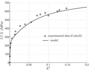
The samples were 140mm long, 12.5mm wide, and 3mm thick laminations. A MTS uniax-ial electrohydraulic machine (displacement controlled) has been used to carry out the uniaxuniax-ial stress-strain Σ(E) behavior of the material. Unloading/reloading tests allowed us to estimate the kinematic X and isotropic R hardenings as a function of the plastic strain Ep _{via a Cottrell’s} method, which is illustrated in Figure 10. The estimation is based on the identification of limits of the yield surface [48]: maximum stress (tensile test) and minimum stress (compression test). Note that this technique requires the yield surface to be exceeded when carrying out the compres-sion test. A strain offset δ must be chosen on the other hand to detect the non linearity associated with the beginning of plastic flow. The offset chosen during experiments was δ= 0.5 × 10−4.

Σ

(M

P

a)

Ε

Figure 10: Experimental loading-unloading cycle for the identification of hardening parameters using the Cottrell’s method.

The experimental magnetic device enabled magnetic measurements on plastically strained samples in the unloaded state or under reloaded tensile stress. It was composed of a primary coil to magnetize the sample, an H-coil for the measurement of the magnetic field, a pick-up coil (B-coil) to measure the electromotive force, and a set of longitudinal and transverse strain gauges stuck on both faces of the sheet to estimate the plastic strain level and measure the (longitudinal and transverse) magnetostrictive behavior. Two ferrite yokes were assembled with the sample to close the magnetic circuit and reduce the macroscopic demagnetizing field and the form effect. Measurements have been first performed on unstrained samples providing the reference magnetic and magnetostrictive state. Measurements have been next performed on samples submitted to an increasing plastic deformation level Ep: at unloaded state first (Σ = 0) and under increasing reloaded stress Σ below the new yield strength. It has been verified that unloading and re-loading remain in the elastic domain.

Magnetic measurements reported hereafter are the anhysteretic magnetic behavior M(H), the longitudinal and transverse anhysteretic magnetostrictive behavior ǫ_//µ(M) and ǫ⊥µ(M), and the hysteretic magnetic behavior M(H) performed at f=0.1Hz. The anhysteretic curves are measured point by point by applying a sinusoidal magnetic field of mean magnitude H, and of exponentially decreasing form [60]. Three plastic deformation levels have been investigated: 0.1%, 1% et 3%. Figure 2 and 3 reported in Section 2.1 refer to the reference anhysteretic and cyclic magnetic and magnetostrictive behaviors of the material. Figure 4 refers to the nominal true stress- true strain behavior of the material.

4.2. Identification of model parameters

4.2.1. Identification of kinematic hardening via the Cottrell’s method and modeling

Figure 11 reports the tensile stress-plastic strain behavior of the material. A high level of kinematic hardening 3/2X is observed in accordance with the strong heterogeneity of the ma-terial. The isotropic hardening R is, on the contrary, negligible (a small decrease of true flow stress Σy+ R is observed). Two stages are highlighted in the evolution of kinematic hardening: a first strong increase that saturates immediately reaching 250MPa. The increase of kinematic hardening is then moderated but remains non linear. At high deformation, the evolution is linear. We choose to model the kinematic hardening by an addition of three terms (54): one Prager linear term X1(55) and two non-linear Armstrong-Frederick terms X2(56) and X3(57) where ˙p indicates the cumulative plastic strain rate (58). Decomposition in two terms (linear and non-linear) is usual. The second non linear term is employed to simulate the rapid kinematic hard-ening evolution at the beginning of strengthhard-ening. Five parameters have to be identified using the experimental data. Table 1 gives optimized values of modeling parameters (using a least square method). Figure 12 shows a comparison between the modeling results and experimental data. Table 2 regroups the value of 3/2X at the plastic strain levels retained for the magnetic measurements. The measurement error for this estimation is about±20MPa in accordance with the discrepancies observed with the model.

X= X1+ X2+ X3 (54) with: ˙ X1= 2 3C1E˙ p (55) ˙ X2= 2 3C2E˙ p − 1 γ2 X2˙p (56) 20

0 0.02 0.04 0.06 0.08 0.1 0.12 0.14 0.16 −100 0 100 200 300 400 500 600 700

Ε

Figure 11: Stress - plastic strain behavior of dual-phase steel - Associated isotropic and kinematic hardening.

C1(MPa) C2(MPa) γ2 C3(MPa) γ3

333 226667 0.00114 6000 0.059

Table 1: Parameters of the kinematic hardening model of dual-phase steel.

˙ X3= 2 3C3E˙ p −_γ1 3 X3˙p (57) with ˙p= √ 2 3E˙ p ∶ ˙Ep (58) Ep 3/2X (MPa) 0.001 100±20 0.01 270±20 0.03 400± 20

Table 2: Estimation of the stress level corresponding to the centre of yield surface (3/2X) at the plastic strain levels retained for the magnetic experiments.

4.2.2. Identification of the magnetic parameters for each phase

As indicated in Section 3.3.2 the multidomain model requires parameters for each phase: ferrite and martensite. The parameter identification needs accurate measurements of the magnetic and magnetostrictive behaviors of both materials taken seperately. The behavior of ferrite is assumed to be very close to the behavior of pure iron. The behavior and physical parameters of

0 0.05 0.1 0.15 0.2 0 100 200 300 400 500 600 700 Εp 3/ 2 X (M P a)

experimental data (Cottrell) model

Figure 12: Measurement and modeling of the kinematic hardening

such a material are well documented. The behavior of the martensitic phase is more difficult to obtain and much less well documented in the literature. Indeed martensite seems to be strongly sensitive to the carbon content, alloying elements and heat treatments [59]. A procedure detailed in [9] allowed us to obtain a fully martensitic steel after an appropriate heat treatment of a 0.4wt% carbon content mild steel (C38 steel). Microhardness and microstructure of DP steel and C38 martensite have been found to be in good agreement. This material is supposed to exhibit the same magneto-mechanical behavior as the martensite phase in the DP steel.

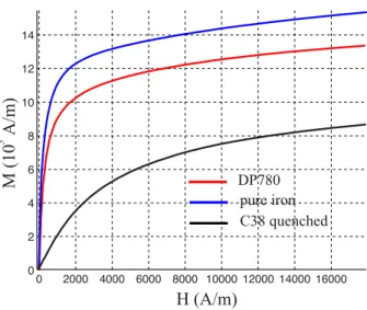
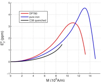
Magneto-mechanical experiments have been performed on a pure iron sample and on a quenched C38 sample following the experimental procedure detailed in Section 4.1. Figures 13 and 14 show the experimental results obtained for magnetic and longitudinal magnetostrictive behavior without an applied stress. As expected, the behavior of DP steel that has been added in the figure is located between the two other behaviors.

The tables below list the parameters used for the modeling of each phase. Physical parame-ters for pure iron are well known (magnetocrystalline and magnetostrictive constants, saturation magnetization). χ0and σcon f are the only parameters optimized to fit properly the magnetization curve for χ0 and the magnetostriction curve for σcon f. Physical parameters of martensite are unable to be found in the literature. An isotropic behavior has been supposed for this second phase that reduces the magnetostrictive parameters to one. Its value is optimized to fit properly the magnetostriction curve. χ0, Msand K1are optimized thanks to the magnetization curve. The magnetocrystalline constant K1has been fixed to a high value to reproduce the high coercivity of the martensite. Mshas then been reduced from the theoretical value of pure iron to properly fit the saturation in the measurement range. The configuration energy has not been considered for this material since the optimization of the magnetostriction saturation value is enough to get an accurate restitution of the behavior. Other fixed parameters are the loading angles of the multido-main modeling (φ, θ) = (38.81○, 77.54○) and Young modulus and Poisson ratio (E,ν) = (200GPa, 0.3).

Once the best parameters describing the ferrite and martensite behavior are found, a dual phase medium can be modeled using volume fractions fs = 0.7 and fh = 0.3. A fixed point

0 2000 4000 6000 8000 10000 12000 14000 16000 2 4 6 8 10 12 14

H (A/m)

M

(10 A

/m

)

Figure 13: Anhysteretic magnetic behavior of DP780 steel, pure iron and C38 quenched steel.

2 4 6 8 10 12 14 0 1 2 3 4 5

M (10 A/m)

Ε

(ppm

)

Figure 14: Anhysteretic magnetostrictive behavior of DP780 steel, pure iron and C38 quenched steel.

method is employed to get the average behavior taking account of the stress and magnetic field localization (convergence is reached after less than 10 loops - computation time is about 2.7 sec-onds per point using MatlabOR

software implemented in a personal computer). Figures 15 and 16 show the modeling results for magnetization longitudinal magnetostriction curves for the three materials. The modeled behavior for DP780 steel is in very good agreement with the experimen-tal behavior. The bigger discrepancies concern the magnetostriction behavior especially for pure iron at intermediate magnetic fields.

Param. Ms K1 λ100;λ111 χ0 σcon f

Value 1.71×106 _{48 21;-21 2000 9}

Unit A/m kJ.m−3 ppm - MPa

Table 3: Parameters of multidomain modeling for iron (s) phase.

Param. Ms K1 λ100;λ111 χ0 σcon f

Value 1.25×106 500 4.8;4.8 150 0

Unit A/m kJ.m−3 ppm - MPa

Table 4: Parameter for martensite (h) phase.

0 2000 4000 6000 8000 10000 12000 14000 16000 0 2 4 6 8 10 12 14 H (A/m) M (1 0 5 A/ m) DP780 pure iron C38 quenched

Figure 15: Modeling results - anhysteretic magnetic behavior of DP780 steel, pure iron and C38 quenched steel.

4.3. Experimental results and modeling 4.3.1. Effect of applied stress - elastic domain

A positive uniaxial stress is applied on the DP steel sample keeping stress below the yield limit. This first test allows to observe the behavior of the material and of the model in a condition where the material is kept in a reversible condition (i.e. X = 0). Experimental and modeling results are plotted successively for a better appreciation of discrepancies. Figure 17a shows the initial state and the effect of stress on the anhysteretic magnetic behavior of the DP steel. The tensile stress has only a moderate influence on the magnetic behavior. This results in a slight increase in the susceptibility before the Villari reversal (beyond 2000 A/m) and a decrease of magnetization after this point, as commonly observed for steels. It can be however noticed that the effect of stress on magnetic susceptibility is non monotonic at high stress intensity. The mag-netic behavior at Σ=200MPa is for example always below the magmag-netic behavior at Σ=150MPa.

0 2 4 6 8 10 12 14 −1 0 1 2 3 4 5 M (105A/m) E µ (p // p m) DP780 pure iron C38 quenched

Figure 16: Modeling results - anhysteretic magnetostrictive behavior of DP780 steel, pure iron and C38 quenched steel.

This counterintuitive phenomenon was already observed in iron-silicon [62] or iron-cobalt al-loys [63], in contradiction with the classical magneto-elastic effect. It was interpreted and mod-eled in a multiscale framework in [62] as an effect of stress on the initial domain configuration (demagnetizing stress e f f ect). Except concerning the non-monotony at high tensile stress (the demagnetizing stress effect is not considered in the present paper), the modeling plotted in Figure 17b and the experiments are in good agreement.

Figure 18a shows the initial state and the effect of stress on the anhysteretic magnetostriction (longitudinal and transverse) of the DP steel. This behavior is clearly much more sensitive to ap-plied stress than the magnetic behavior. The modeling plotted in Figure 18b gives results in very good agreement with experiments. The saturation level of magnetostriction is however higher for the modeling (from 4.5ppm for experiments to 5.8ppm for modeling at 200MPa). This differ-ence has to be related to the shift procedure applied to the experimental data as explained in [61]. The plot of experimental and modeled ∆E effect in Figure 19 extracted from magnetostriction results allows an illustration of this point. These results show finally the ability of the model to reproduce the effect of stress on the magnetic and magnetostrictive behaviors of the DP steel. It is a prerequisite for modeling the influence of plasticity via a magnetoelastic approach.

0 1000 2000 3000 4000 5000 6000 0 2 4 6 8 10 12 0MPa 25MPa 50MPa 100MPa 200MPa

H (A/m)

M

(10 A

/m

)

Figure 17: Influence of tensile applied stress below yield strength on the anhysteretic magnetic behavior of DP780 steel.

−10 − 5 0 5 10 −3 −2 −1 0 1 2 3 4 5 6 _{0 MPa} 25 MPa 50 MPa 200 MPa 100 MPa Longitudinal Transverse 5 M (10 A/m)

Ε

(ppm

)

Figure 18: Influence of tensile applied stress below yield strength on the anhysteretic magnetostrictive behavior of DP780 steel - Longitudinal: deformation measured in the direction of applied field; Transverse: deformation measured perpendicularly to the direction of applied field.

0 50 100 150 200 250 −3 −2 −1 0 1 2 3 4 5 6 Σ (MPa) E µ (p p m) Longitudinal Tranverse / / Experiments Modeling

Figure 19: Comparison model/experiments of anhysteteric longitudinal and transverse ∆E effect for DP780 steel (ex-tracted from results plotted in Figures 18a and 18b).

4.3.2. Effect of plastic straining on the magnetic and magnetostrictive behaviors

Three different specimens of DP780 steel has been deformed up to 0.1%, 1% and 3% (i.e. Ep= 0.001, Ep= 0.01 and Ep= 0.03). Their magnetic and magnetostrictive behaviors have been measured after plastic deformation at unloaded state first, under applied tensile test next. The uniaxial stress introduced in the modeling of each phase (s: ferrite; h: martensite) is defined by:

σeq_s = Σ −3 2X+ E(7 − 5ν) 10(1 − ν2)(E µ− ǫµ s) σ eq h = Σ + fs fh 3 2X+ E(7 − 5ν) 10(1 − ν2)(E µ− ǫµ h) (59)

where 3/2X depends on the plastic strain level. Values are reported in the previous Table 2 and come from the Cottrell analysis. The following assumptions are consequently made:

• isotropic distribution of the two phases in the material;

• isotropic distribution of crystallographic orientations in each phase; • behavior of each phase supposed unchanged with plastic strain.

The last assumption is maybe the weakest because we know that plasticity of the soft phase (ferrite in the present case) is associated with a significant change of dislocation density that may change the behavior of the phase. This contribution is not considered in the modeling.

Figure 20a shows the effect of the three plastic strain levels on the magnetic behavior at un-loaded state (Σ = 0). A strong non linear degradation is observed as reported by many authors in previous works. The corresponding modeling is plotted in Figure 20b giving results in good agreement with experimental ones. Figure 21a and 22a report the associated magnetostrictive be-havior (along longitudinal and transverse directions respectively). The plastic strain acts clearly as a compressive stress effect as foreseen by the theoretical approach. Modelings reported in Figure 21b and 22b give results in good qualitative agreement with experiments. The shape of

the magnetostriction curves at Ep= 0.03 nevertheless exhibits some inflexions that do not seem physical. This defect is due to the strong simplifications of the multidomain modeling leading to an dissymmetric rotation of the magnetic moments under stress. This defect disappears when the full multiscale modeling is employed to model the behavior of each phase. The computation time is however thousand of times longer for a relatively small improvement.

As a conclusion of this part, it is possible to confirm that the modeling of the effect of plastic strain on the magnetic behavior through a purely mechanical description (introduction of residual stress field) is possible and gives some very accurate results for plastic straining up to 3%.

0 2000 4000 6000 8000 0 2 4 6 8 10 12 5 H (A/m) M (10 A /m ) p = 0.001 p = 0.01 p = 0.03 Εp= 0 reference Ε Ε Ε (a) Experiments 0 2000 4000 6000 8000 0 2 4 6 8 10 12 H (A/m) M (1 0 5 A/ m) reference Ep=0.001 Ep=0.01 Ep=0.03 (b) Modeling

Figure 20: Anhysteretic magnetic behavior of plastic strained samples at unloaded state.

−1 −0.5 0 0.5 1 1.5 − 8 −6 −4 −2 0 2 M (106_A/m) p = 0.001 p = 0.01 p = 0.03 Εp = 0 µ

E

Figure 21: Longitudinal anhysteretic magnetostrictive behavior of plastic strained samples at unloaded state.

M (106A/m) µ

E

Figure 22: Transverse anhysteretic magnetostrictive behavior of plastic strained samples at unloaded state.

4.3.3. Effect of plastic straining: reloaded state

The plastically strained samples are submitted to an increasing level of tensile stress (remain-ing in the ”new” elastic domain). The model(remain-ing is obtained by us(remain-ing an increas(remain-ing value of Σ in equation (59). Magnetization, longitudinal and transverse magnetostrictive measurements are performed. Figures 23a, 24a and 25a show the evolution of the magnetic behavior of the sample plastic strained at 0.1%, 1% and 3% respectively and reloaded at various stress levels indicated in the figures. Figures 23b, 24b and 25b plot the associated modelings. It is remarkable to ob-serve that the reloading allows to progressively recover the reference (Ep= 0 and Σ = 0) behavior whatever the plastic strain level. This behavior is in agreement with the residual stress origin of the initial degradation associated with plastic strain. Indeed, as explained before, the residual stress in the s phase (σs

eq≈ Σ − 3/2X) that mostly contributes to the average magnetic behavior, becomes positive for Σ > 3/2X. If the influence of the second phase (lower quantity and lower sensitivity to stress) is negligible, the reference behavior could be reached for an applied stress value theoretically close to 3/2X value. Experimental results are roughly in accordance with this interpretation. This conclusion seems less clear for the 0.1% strained sample where the tested re-loaded stress levels are insufficient. Since the modeling is built using the same principles, it allows a good restitution of the effect of a superimposed applied stress. Particularly, the reference behavior is clearly reached for a stress value close to 3/2X that confirms the moderated role of the second phase. This stress denoted Σχcis called ”magnetic recovery stress”. We observe neverthe-less that the modeled magnetic behaviors clearly overstep the reference behavior at high stress. This is not observed in the experiments; it should probably be related to the non-monotonic effect of tensile stress already observed but not considered in the modeling.

102 103 2 4 6 8 10 12 H (A/m) 380 MPa 180 MPa 0 MPa 60 MPa 5 M (10 A /m ) Reference (a) Experiments 102 103 0 2 4 6 8 10 12 H (A/m) M (1 0 5 A/ m) 380 MPa 180 MPa 0 MPa 60 MPa Reference (b) Modeling

Figure 23: Anhysteretic magnetic behavior of the sample plastic strained at 0.1% and reloaded at various stress levels.

102 103 2 4 6 8 10 12 0 MPa 80 MPa 200 MPa 250 MPa 300 MPa 350 MPa 450 MPa 490 MPa Reference 5 H(A/m) M (10 A /m ) (a) Experiments 102 103 0 2 4 6 8 10 12 H (A/m) M (1 0 5 A/ m) 0 MPa 80 MPa 200 MPa 250 MPa 300 MPa 350 MPa 450 MPa 490 MPa Reference (b) Modeling

Figure 24: Anhysteretic magnetic behavior of the sample plastic strained at 1% and reloaded at various stress levels.

10 2 10 3 2 4 6 8 10 12 5 H(A/m) M (10 A /m ) Reference 452 MPa 372 MPa 480 MPa 586 MPa 0 MPa 80 MPa 160 MPa 215 MPa 266 MPa 319 MPa 532 MPa (a) Experiments 102 103 0 2 4 6 8 10 12 H (A/m) M (1 0 5 A/ m) Reference 452 MPa 372 MPa 480 MPa 586 MPa 0 MPa 80 MPa 160 MPa 215 MPa 266 MPa 319 MPa 532 MPa (b) Modeling

Figure 25: Anhysteretic magnetic behavior of the sample plastic strained at 3% and reloaded at various stress levels.

Figure 26 plots the initial susceptibility χ0 = (dM/dH)H=0of the non-deformed and plasti-cally strained samples as a function of the applied stress for the experiments and modeling. Even if the magnetic behavior cannot be summarized by χ0, this plot allows an easy observation of the effects detailed above. The magnetic recovery stress Σχc is clearly identifiable, as the non-monotonic effect is not reproduced by the modeling. It can be noticed that the global level of initial susceptibility predicted by the model is lower than the experimental susceptibility. This probably comes from the underestimation of the initial susceptibility of the ferrite phase.

Figures 27-32a show the evolution of the longitudinal and transverse magnetostrictive be-haviors of the sample plastic strained at 0.1%, 1% and 3% respectively and reloaded at various stress levels indicated in the figures. Figures 27-32b plot the associated modelings in good global

0 100 200 300 400 500 600 500 1000 1500 2000 2500 3000 Σ (MPa) χ 0 p = 0 p = 0.001 p = 0.01 p = 0.03 E E _E E (a) Experiments 0 100 200 300 400 500 600 700 500 1000 1500 2000 Σ (MPa) χ 0 p = 0 p = 0.001 p = 0.03 E E E p = 0.01 E (b) Modeling

Figure 26: Initial susceptibility of the samples as function of the reloaded stress.

agreement with the experiments. As for the magnetic behavior, a critical stress allows to recover the initial magnetostrictive behavior of the material. This ”magnetostriction recovery stress” is denoted Σχc and values are close to 3/2X as observed for the magnetic behavior. Below Σµc, the material behaves like an unstrained material submitted to a compression. Above Σµc, the mate-rial behaves like an unstrained matemate-rial submitted to tensile stress. The phenomenon reaches a saturation stage at higher levels of applied stress.

−1.5 −1 −0.5 0 0.5 1 1.5 −6 −4 −2 0 2 4 6 8 380 MPa 180 MPa 60 MPa 0 MPa

M (10

A/m)

E

(ppm

)

Figure 27: Anhysteretic longitudinal magnetostrictive behavior of the sample prestrained at 0.1% and reloaded at various stress levels.

−1 −0.5 0 0.5 1 1.5 −4 −3 −2 −1 0 1 2 3 E (pp m ) 380 MPa 180 MPa 60 MPa 0 MPa ⊥ µ M (106A/m) reference (a) Experiments −1.5 −1 −0.5 0 0.5 1 1.5 −4 −3 −2 −1 0 1 2 3 M (106A/m) E µ (p ⊥ p m) reference 380 MPa 180 MPa 60 MPa 0 MPa (b) Modeling

Figure 28: Anhysteretic transverse magnetostrictive behavior of the sample prestrained at 0.1% and reloaded at various stress levels.

−1.5 −1 −0.5 0 0.5 1 1.5 −6 −4 −2 0 2 4 6 8 80 MPa 490 MPa 400 MPa 350 MPa 300 MPa 250 MPa 200 MPa 0 MPa

M (10

A/m)

E

(ppm

)

Figure 29: Anhysteretic longitudinal magnetostrictive behavior of the sample prestrained at 1% and reloaded at various stress levels.