HAL Id: inserm-00255894
https://www.hal.inserm.fr/inserm-00255894
Submitted on 14 Feb 2008HAL is a multi-disciplinary open access archive for the deposit and dissemination of sci-entific research documents, whether they are pub-lished or not. The documents may come from
L’archive ouverte pluridisciplinaire HAL, est destinée au dépôt et à la diffusion de documents scientifiques de niveau recherche, publiés ou non, émanant des établissements d’enseignement et de
3-D Modeling of the Thermal Coagulation Necrosis
Induced by an Interstitial Ultrasonic Transducer.
Carole Garnier, Cyril Lafon, Jean-Louis Dillenseger
To cite this version:
Carole Garnier, Cyril Lafon, Jean-Louis Dillenseger. 3-D Modeling of the Thermal
Coagula-tion Necrosis Induced by an Interstitial Ultrasonic Transducer.. IEEE TransacCoagula-tions on Biomed-ical Engineering, Institute of ElectrBiomed-ical and Electronics Engineers, 2008, 55 (2), pp.833-837. �10.1109/TBME.2007.914543�. �inserm-00255894�
3D Modeling of the Thermal Coagulation Necrosis Induced by an
Interstitial Ultrasonic Transducer
Carole Garnier*,** Cyril Lafon***,**** Jean-Louis Dillenseger*,**
From:
* INSERM, U642, Rennes, F-35000, France;
** Universit´e de Rennes 1, LTSI, Rennes, F-35000, France; *** INSERM, U556, Lyon, F-69003 France.
**** Universit´e Claude Bernard Lyon 1, Lyon, F-69000 France. Corresponding author:
Jean-Louis Dillenseger
Laboratoire Traitement du Signal et de l’Image, INSERM U642, Universit´e de Rennes I,
Campus de Beaulieu, 35042 Rennes Cedex, France. tel: +33 (0)2 23 23 55 78 fax: +33 (0)2 23 23 69 17 email: Jean-Louis.Dillenseger@univ-rennes1.fr
Abstract
This paper describes a temperature-varying attenuation approach for pre-operative planning of high intensity ultrasound interstitial targeted therapy. Such approach is mainly aimed at the treatment of primary liver cancer for which a precise lesion control must be achieved. It is shown through simulation that the shape and size of the resulting necrotic volume is significantly different from the one obtained when this tissue property is considered constant in time.
Index terms
High intensity ultrasound therapy, hyperthermia, interstitial therapy, planning, simulation, tis-sue properties.
1
Introduction
Hepatocellular carcinoma or primary liver cancers lead to more than 1 million new cases diag-nosed each year. Although less common in the western countries, its incidence is rising [1]. At early stages, hepatocellular carcinoma is confined to a solitary mass and is therefore potentially curable by surgical resection [2]. However, tumors can be localized but unresectable due to critical anatomical environment, concomitant disease such as cirrhosis or even bilateral loca-tions. These patients may then undergo percutaneous surgery (percutaneous ethanol injection, or radiofrequency) [3]. An alternative based on high intensity ultrasound therapy is proposed using a similar interstitial approach [4]. Interstitial ultrasound offers the advantage to be more controllable in depth and direction than other interstitial heating modalities. Like any other minimally invasive image guided therapy, its clinical application requires an efficient planning at the pre-operative stage, and an accurate tracking and control during the intra-operative phase. Thus, in addition to the classical image processing issues (segmentation, registration,
HAL author manuscript inserm-00255894, version 1
HAL author manuscript
rendering, etc.), a sound physically-based model of the thermal dose to be delivered must be designed that should be updated according to the temperature measurements when the inter-vention is performed. A first computer simulation tool for high energy ultrasound therapy has been reported in [5] which relied on tissue spatial homogeneity and invariance of its acoustic properties. However, this tool proposed an exact pressure field estimation. More recently, Mast et al [6] proposed an enhanced model, but with a planar transducer geometry limitation and mathematical simplifications, which have an influence on the pressure field computation espe-cially close to the simulated transducer. To go further, we propose a model which relies on a balance between complexity and computation time. In this paper, we introduce time-varying properties of the tissue during ultrasound application together with accelerated techniques for dose computation. Section 2 provides the basic features of the model and Section 3, an example illustrating the difference in the necrotic size estimation that can be observed between invariant and variable tissue properties hypotheses.
2
Method
2.1 Transducer geometry and control
The modeled therapeutic ultrasound device (Fig. 1) was composed of a small (3 mm x 10 mm) planar ultrasonic mono-element transducer encapsulated in a cylindrical interstitial applicator. The transducer operated at a single frequency between a range from 5 to 15 MHz depending on its geometrical design. The transducer was air-backed, so ultrasound was only propagated forward. The front transducer face was cooled by a continuous flow of degassed water maintained at a constant temperature (5˚C in the therapeutic case) . The therapy consisted in a sequence of exposures. After each exposure the applicator was rotated by a specific angle in order to deposit heat according to the tumor geometry. The planning parameters are the exposure duration; the ultrasonic intensity (measured by a force balance at the surface of the applicator); the angular step between two adjacent elementary exposures and the total angle of treatment.
2.2 Computer simulation
The modeling can be summarized as follows:
1. Each shot produces a pressure field p. The calculated pressure field depends on the physical and the tissue assumptions. This point will be addressed in section 2.3.
2. The energy of the beam is converted into heat. The tissue temperature evolution over time is obtained by solving Pennes’ bioheat transfer equation (BHTE) [7] which describes thermal processes in human perfused tissues. The BHTE has the following 3D+t form:
ρtCt
∂T
∂t = kt∇
2T + V ρ
bCb(Ta−T ) + Q (1)
where T is the temperature and ρt, Ct, kt, V , ρb, and Cb are respectively the density, the
specific heat and thermal conductivity of tissues, the perfusion rate per unit volume of tissues, the density and the specific heat of blood. This equation describes the variation of energy per unit of volume. In (1), it can be seen that this variation can be divided into three terms (from left to right): the thermal diffusion, the effect of perfusion and Q the acoustic power provided by the exposures. Q is directly deduced from the simulated
pressure field (Q ∝ p2). A finite difference method was used to solve this equation [8]. The
temperature of the cooling water serves as an iso-thermal boundary condition. As ebul-lition was not considered in the present model and for avoiding unrealistic temperatures; a threshold ensures that the temperature could never exceed 100˚C. We take also the tissue necrosis into account: the perfusion rate V is set to zero when tissues are necrosed.
3. The concept of thermal dose [9], which is quite standard in tumor hyperthermia literature, was used to assess thermal damages. For each location and history of temperature, the thermal dose is defined as an equivalent time the temperature of reference of 43˚C should be applied to obtain the same thermal damage. It can be computed directly from the temperature map: D43˚C(x, y, z, t) = t X i=1 R(43−T (x,y,z,t))∆t (2)
with R = 0.5 if T > 43˚C and R = 0.25 otherwise.
4. Liver tissues are considered as irreversibly thermally damaged when D43˚C > 340
min-utes [10].
2.3 Calculation of the pressure field
The determination of the pressure field is one major feature of the overall process. Numerical methods for estimating the pressure field can take into account the nonlinear propagation of high intensity waves [11, 12, 13] or remain purely linear. In our study, with a non-focused plane transducer, the propagation can be considered linear [14]. From this assumption, the pressure field can be exactly computed for the entire volume on the basis of the Rayleigh integral with O’Neil’s hypotheses [5]. The goal is thus to compute the acoustic pressure at a location point M ; the transducer of surface S is sampled into elements of surface ∆S which size is negligible in comparison with the wavelength λ ; M and one element of surface ∆S are connected by a straight segment ∆SM of length l sampled into elements ∆l. The pressure at a location M is given by the discrete version of the Rayleigh integral:
p(M ) = X S jp0 λ∆S exp−j kl l exp −fP l i=1αi∆l (3)
with p0 the pressure at the transducer surface (Pa), k the wave number (2π/λ), f the
transducer frequency (Hz) and αi the tissue attenuation coefficient at location i along the line
segment ∆SM (Np · cm−1·MHz−1).
This twofold integration (over the surface of the transducer and the segment ∆SM ) is very computation intensive. Some simplifications are usually made in order to accelerate the simulation [5]: the tissues are assumed to be homogeneous around the applicator and its physical properties (the tissue attenuation coefficient) constant in time. They have the three following benefits:
• The propagation of a wave from one element of surface ∆S to M is carried through only
2 media: the cooling water of the transducer (α1, l1) and the tissues (α2, l2). Because
α1 is negligible and p0 is estimated at the surface of the applicator, the equation (3) can
therefore be simplified as:
p(M ) = X S jp0 λ∆S exp−j kl l exp −f α2l2 (4)
• The simulated air-backed transducer providing only forward waves and the homogeneous
medium of propagation allow computing pressure in a quarter of a space in front of the propagation axis only for symmetry reasons.
• Regardless to the applicator orientation, the generated pressure field remains constant in the transducer coordinates system. So, the pressure field generated after the rotation of the applicator can simply be obtained by an angular shift of the first estimated pressure field matrix. The necrosis simulation can be summarized as : 1) estimation of the pressure field for one exposure; 2) temporal integration of this pressure field within the BHTE (1) after rotation by the planned angles.
Adaptative sampling of the transducer and volume of calculation allows a relatively fast pressure field computation time (8 minutes on a conventional PC: AMD Athlon 2200+ proc. with 1MB RAM).
2.4 Dynamic tissue attenuation coefficient variation
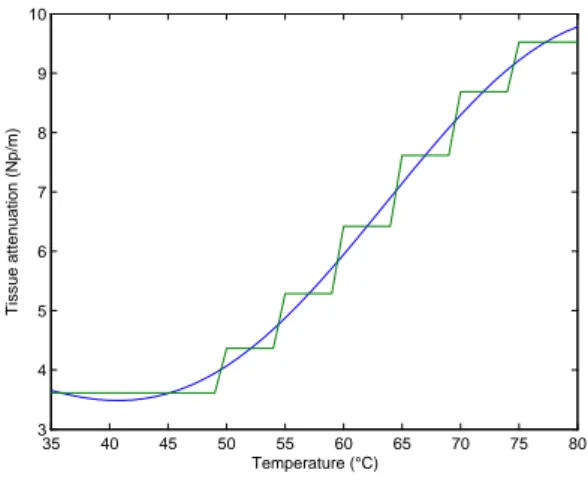
The attenuation coefficient associated to a given tissue is no more constant over time. This coefficient changes as temperature changes and as tissue necroses. The attenuation coefficient curves (ie coefficient variation vs. temperature) was measured for various tissues [15]. For liver, Connor et al. [13] made a 6th order polynomial approximation of the experimental data (see curve in Fig. 2).
Taking this attenuation coefficient variation into account modifies the simulation framework described in section 2.2: 1) the pressure field is first computed and then incorporated into the BHTE; 2) according to the computed temperatures, the tissue attenuation coefficients at each location of the volume are updated; 3) a new pressure field is then estimated and so on.
The consequence of this time-varying behavior is that the hypothesis of homogeneity and time invariance of the tissue properties is no more true. The three previous described simpli-fications (analytical integration simplification of (4), symmetry and pressure field invariance) cannot be used anymore. The brute force algorithm based on (3) induces a tremendous comput-ing time for the overall necrosis estimation. However, several simplifications can be proposed in order to reasonably reduce this computing time without loosing accuracy on the estimate of the necrosed volume:
• Within the BHTE, the temperature variation is relatively slow, so the tissue attenuation
coefficient variation is slow too. Two different time steps can be considered: a fast one (∆t = 0.02s) for resolving the BHTE (1) and a longer one (2s) for updating the attenuation coefficients and the pressure field.
• The tissue attenuation coefficient curves is stepwise approximated (Fig 2). This allows to
cluster the volume elements into larger regions with constant tissue coefficients. The
seg-ment ∆SM crosses now regions with a constant attenuation coefficient αi over a distance
li. Equation 3 can then be rewritten as:
p(M ) = X S jp0 λ∆S exp−j kl l exp −f PN i=1αili (5) Where N denotes the number of crossed regions along the segment ∆SM .
• Segment coherence was also considered: adjacent ∆SM segments share almost the same
attenuation properties. For nine adjacent connected transducer surface element ∆S, we
compute the exp−f
PN
i=1αiliterm of equation 5 for only the ∆SM segment which originates
from the central surface element and apply this term to the segments which originate from the eight adjacent surface elements.
These simplifications, with the volume and transducer adaptive sampling mentioned in sec-tion 2.3, allow reducing the computasec-tion time to around 16h30. Some optimizasec-tions are still under study in order to keep diminishing the computation time.
2.5 Experimental validation of the model
For comparison, an experiment was performed in vivo [4]. The transducer was positioned inside the liver of a pig, away from large blood vessels. This animal experimentation was approved by a veterinarian ethics committee. At the time of the study we only had at our disposal a 10.7 MHz
transducer. The exposure conditions were set to: 14 W/cm2 for the intensity measured by a
force balance at the surface of the applicator; 37˚C for the transducer cooling water temperature and 20 s for the duration of the exposure. Four thermocouples were introduced inside liver on the acoustic axis of the transducer right at the end of the 20 s-long exposure. The maximum increase of temperature was measured at four different positions: 2.5, 5, 7.5 and 10 mm from the applicator surface.
3
Results and Discussion
Our goal is to simulate a real therapy. In order to maximize the necrotic volume size, we choose
to develop a 5 MHz therapeutic ultrasound device with an intensity of 40 W/cm2 measured by
a force balance at the surface of the applicator and a constant cooling water temperature of 5˚C. The simulated therapy strategy consisted of a sequence of twenty six 3 s-long exposures. The transducer was rotated by 3.6˚after each exposure. Thus, the device swept a 90˚angle. The tissues, perfusion and blood parameters were found in the literature [16, 17, 18].
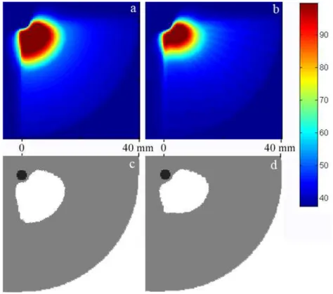
Fig. 3 shows the maximum temperature field obtained during the sequence (3-a and 3-b) and the obtained necrotic volume final form (3-c and 3-d) in an axial XY cut plan at z = 0 (see the coordinates system on Fig. 1). Figures 3-a and 3-c were obtained considering homogeneous tissues (4) while figures 3-b and 3-d included the variation of attenuation coefficients with temperature (5).
The simulations point out that the obtained maximal temperatures increased higher and faster near the transducer when the attenuation varied with temperature. The attenuation coefficient increased principally over a limited depth, close to the transducer, where heating is more intense. Most of the acoustic power is then absorbed near the transducer with the effect to decrease the available power deposit at more distant regions. The consequence is that the proximal heating is enhanced even more and the distal heating is decreased. Furthermore the size of the necrotic volume is naturally reduced in the direction of propagation. This can be observed on Fig. 3: the temperature field, the thermal dose field and so the necrotic volume were less extended in the radial direction. This observation is particularly true at the end of the movement of the transducer (Θ = 90˚). In the radial distance form the transducer, the necrotic volume reaches a distance of 15 mm when attenuation coefficient is constant, but only 11 mm when the necrotic volume is estimated using the temperature dependent attenuation coefficient. Some changes can also be noticed along the Z axis where the temperature field and so the necrotic volume are less extended of about 2 mm on that direction when coefficients vary with temperature. The dissymmetrical shape of the necrosis is due to the fact that the increase of temperature in tissues is still low for the first elementary exposures, while successive exposures benefit from previous exposures. Consequently, the decrease in the necrotic volume size, for higher rotation angle of treatment, is more substantial because of higher attenuation coefficients.
These facts are confirmed by the experimental validation of the model presented on sec-tion 2.5. Fig. 4 compares the real temperatures measured on the in vivo experimental validasec-tion at the four different positions and the temperature curves obtained by the two simulation meth-ods initialized by the parameters of the experimental protocol described in [4]. The temperature curve obtained by the approach using attenuation coefficient variation with temperature is closer to the experimental data.
This approach, that takes into account the variation of attenuation with temperature, shows
significant changes in both the size and the shape of the necrotic volume. Therefore and in spite of the computing time, it is important to integrate this phenomenon and other complex tissue properties into the model (vascular structures proximity, vaporization...). Defining and opti-mizing the planning parameters with accuracy would permit to obtain a more precise adapted therapy. The next step would be to run more experiments that are relevant to the treatment strategy (juxtaposition of elementary exposures) in order to validate the model. The comparison could be based on the in vivo macroscopic evaluation of the thermal lesion or on temperature maps recorded during treatment by MRI [19, 20].
4
Conclusion
A method simulating the formation of necrosis generated by high intensity ultrasound was described. The classical model assumed that tissues are homogeneous with physical properties invariant during the treatment. Instead of that assumption, we introduced a new model which takes into account the variation of the tissue attenuation coefficient. This method predicts the size and shape of the necrotic volume with a better accuracy and so allows a more precise therapy planning.
5
Acknowledgements
This work is part of the national SUTI project supported by an ANR Grant (ANR05RNTS01106). The authors would like to thank J.-L. Coatrieux for his advices in conducting this research project and his contributions in writing this paper.
References
[1] H. B. El-Serag and A. C. Mason, “Rising incidence of hepatocellular carcinoma in the United States,” N Engl J Med, vol. 340, no. 10, pp. 745–50, 1999.
[2] E. Mor, R. T. Kaspa, P. Sheiner, and M. Schwartz, “Treatment of hepatocellular carcinoma associated with cirrhosis in the era of liver transplantation,” Ann Intern Med, vol. 129, no. 8, pp. 643–53, 1998.
[3] R. A. Lencioni, H. P. Allgaier, D. Cioni, M. Olschewski, P. Deibert, L. Crocetti, H. Frings, J. Laubenberger, I. Zuber, H. E. Blum, and C. Bartolozzi, “Small hepatocellular carcinoma in cirrhosis: randomized comparison of radio-frequency thermal ablation versus percuta-neous ethanol injection,” Radiology, vol. 228, no. 1, pp. 235–40, 2003.
[4] C. Lafon, J. Y. Chapelon, F. Prat, F. Gorry, J. Margonari, Y. Theillere, and D. Cathig-nol, “Design and preliminary results of an ultrasound applicator for interstitial thermal coagulation,” Ultrasound Med Biol, vol. 24, no. 1, pp. 113–22, 1998.
[5] C. Lafon, F. Prat, J. Y. Chapelon, F. Gorry, J. Margonari, Y. Theillere, and D. Cathig-nol, “Cylindrical thermal coagulation necrosis using an interstitial applicator with a plane ultrasonic transducer: in vitro and in vivo experiments versus computer simulations,” Int J Hyperthermia, vol. 16, no. 6, pp. 508–22, 2000.
[6] T. D. Mast, I. R. Makin, W. Faidi, M. M. Runk, P. G. Barthe, and M. H. Slayton, “Bulk ablation of soft tissue with intense ultrasound: modeling and experiments,” J Acoust Soc Am, vol. 118, no. 4, pp. 2715–24, 2005.
[7] H. H. Pennes, “Analysis of tissue and arterial blood temperatures in the resting human forearm. 1948,” J Appl Physiol, vol. 85, no. 1, pp. 5–34, 1998.
[8] J. Chato, M. Gautherie, K. Paulsen, and R. Roemer, Thermal dosimetry and treatment planning, ch. Fundamentals of bioheat transfer, pp. 1–56. Berlin: Springer, 1990.
[9] S. A. Sapareto and W. C. Dewey, “Thermal dose determination in cancer therapy,” Int J Radiat Oncol Biol Phys, vol. 10, no. 6, pp. 787–800, 1984.
[10] S. J. Graham, L. Chen, M. Leitch, R. D. Peters, M. J. Bronskill, F. S. Foster, R. M. Henkelman, and D. B. Plewes, “Quantifying tissue damage due to focused ultrasound heating observed by MRI,” Magn Reson Med, vol. 41, no. 2, pp. 321–8, 1999.
[11] P. M. Meaney, M. D. Cahill, and G. R. ter Haar, “The intensity dependence of lesion position shift during focused ultrasound surgery,” Ultrasound Med Biol, vol. 26, no. 3, pp. 441–50, 2000.
[12] V. A. Khokhlova, R. Souchon, J. Tavakkoli, O. A. Sapozhnikov, and D. Cathignol, “Nu-merical modeling of finite-amplitude sound beams: Shock formation in the near field of a cw plane piston source,” J Acoust Soc Am, vol. 110, no. 1, pp. 95–108, 2001.
[13] C. W. Connor and K. Hynynen, “Bio-acoustic thermal lensing and nonlinear propagation in focused ultrasound surgery using large focal spots: a parametric study,” Phys Med Biol, vol. 47, no. 11, pp. 1911–28, 2002.
[14] F. A. Duck, “Nonlinear acoustics in diagnostic ultrasound,” Ultrasound Med Biol, vol. 28, no. 1, pp. 1–18, 2002.
[15] C. A. Damianou, N. T. Sanghvi, F. J. Fry, and R. Maass-Moreno, “Dependence of ultrasonic attenuation and absorption in dog soft tissues on temperature and thermal dose,” J Acoust Soc Am, vol. 102, no. 1, pp. 628–34, 1997.
[16] F. Dunn and W. D. O’Brien, Ultrasonic biophysics, vol. 7 of Benchmark papers in acoustics. Stroudsburg (Pennsylvania): Dowden-Hutchinson & Ross Inc., 1976.
[17] Task group report of the european society for hypermermic oncology, “Treatment planning and modeling in hyperthermia,” 1992.
[18] P. Bioulac-Sage, B. Le Bail, and C. Balaudaud, “Histologie du foie et des voies biliaires,” in H´epathologie clinique (J. Benhamou, J. Bircher, N. McIntyre, M. Rizetto, and J. Rodes, eds.), pp. 12–20, Paris: Med. sciences/Flammarion, 1993.
[19] R. V. Mulkern, L. P. Panych, N. J. McDannold, F. A. Jolesz, and K. Hynynen, “Tissue temperature monitoring with multiple gradient-echo imaging sequences,” J Magn Reson Imaging, vol. 8, no. 2, pp. 493–502, 1998.
[20] S. L. Hokland, M. Pedersen, R. Salomir, B. Quesson, H. Stodkilde-Jorgensen, and C. T. Moonen, “MRI-guided focused ultrasound: methodology and applications,” IEEE Trans Med Imaging, vol. 25, no. 6, pp. 723–31, 2006.
List of Figures
1 Transducer geometry. . . 8
2 Continuous and stepwise linearized tissue attenuation coefficient vs. temperature. 8
3 Temperature pattern and necrotic volume obtained with the tissue homogeneity
hypotheses (a and c) and attenuation coefficient variation with temperature (b
and d). Temperature scale in ˚C. . . 9
4 Comparison between the experimental in vivo temperature measurements and
the simulated temperatures obtained with the tissue homogeneity hypotheses
and attenuation coefficient variation with temperature. . . 9
Figure 1: Transducer geometry. 35 40 45 50 55 60 65 70 75 80 3 4 5 6 7 8 9 10 Temperature (°C) Tissue attenuation (Np/m)
Figure 2: Continuous and stepwise linearized tissue attenuation coefficient vs. temperature.
Figure 3: Temperature pattern and necrotic volume obtained with the tissue homogeneity hypotheses (a and c) and attenuation coefficient variation with temperature (b and d). Tem-perature scale in ˚C. 0 5 10 15 20 25 30 35 40 35 40 45 50 55 60 65 70 75
Distance from the applicator axis (mm)
Temperature (°C)
In vivo measurements (means and stdv) Tissue homogeneity hypothese Attenuation varying with temperature
Figure 4: Comparison between the experimental in vivo temperature measurements and the simulated temperatures obtained with the tissue homogeneity hypotheses and attenuation co-efficient variation with temperature.