The choice of V/STOL transportation for the Northeast Corridor

-vmlnk

THE CHOICE OF V/STOL

TRANSPORTATION FOR

THE NORTHEAST CORRIDOR

MIT Libraries

Document Services

DISCLAIMER OF QUALITY

Due to the

condition

of the original material, there are unavoidable

flaws in this reproduction. We have made every effort possible to

provide you with the best copy available. If you are dissatisfied with

this product and find it unusable, please contact Document Services as

soon as possible.

Thank you.

.

Page 50 is missing from this

MASSACHUSETTS INSTITUTE OF TECHNOLOGY

Flight Transportation Laboratory

Report FTL - R72 - 2

The Choice of V/STOL Transportation for the Northeast Corridor

William M. Swan June 1972

Abstract

Aircraft type, aircraft size, number of terminals, and degree of nonstop routing for a V/STOL transportation system

in the Northeast Corridor are chosen by exploring a wide range of combinations. Helicopter and STOL aircraft from 20 to 200

seats are considered. From 15 to 20 total terminals were considered. Nonstop, one stop and two stop routings were used. A market model explores the response of a typical route

to variations in these parameters. Demand response to the total trip cost, trip time, and frequency of service is measured by a modal split model. It is found that land costs and manoeuvre times make STOL operations less attractive than VTOL. The system is found to be sensitive to indirect operat-ing costs associated with ticketoperat-ing and boardoperat-ing. A small number of terminals is required. A 16 port system serving

10 cities using a 60 seat helicopter can carry 16% of the

1985 intercity traffic while charging the full costs to the

user. The results were confirmed by a market by market analysis for the corridor.

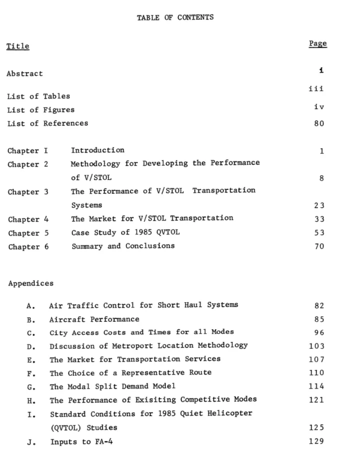
TABLE OF CONTENTS Title Abstract List of Tables List of Figures List of References Chapter I Chapter 2 Chapter 3 Chapter 4 Chapter 5 Chapter 6 Introduction

Methodology for Developing the Performance of V/STOL

The Performance of V/STOL Transportation Systems

The Market for V/STOL Transportation Case Study of 1985 QVTOL

Summary and Conclusions

Appendices

A. Air Traffic Control for Short Haul Systems

B. Aircraft Performance

C. City Access Costs and Times for all Modes

D. Discussion of Metroport Location Methodology

E. The Market for Transportation Services

F. The Choice of a Representative Route

G. The Modal Split Demand Model

H. The Performance of Exisiting Competitive Modes

I. Standard Conditions for 1985 Quiet Helicopter

(QVTOL) Studies J. Inputs to FA-4 Page iii 82 85 96 103 107 110 114 121 125 129

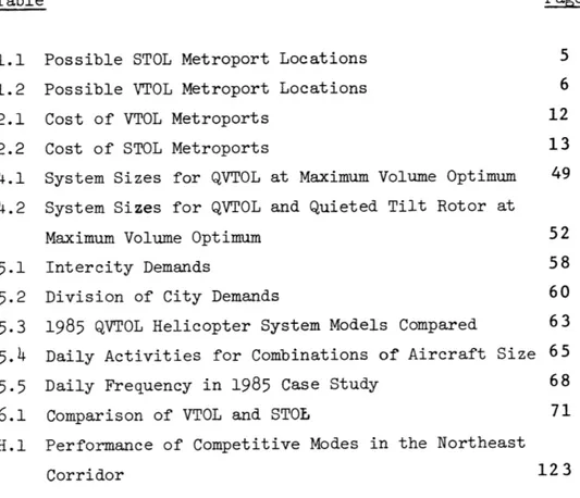
LIST OF TABLES

Table Page

1.1 Possible STOL Metroport Locations 5

1.2 Possible VTOL Metroport Locations 6

2.1 Cost of VTOL Metroports 12

2.2 Cost of STOL Metroports 13

4.1 System Sizes for QVTOL at Maximum Volume Optimum 49

4.2 System Sizes for QVTOL and Quieted Tilt Rotor at

Maximum Volume Optimum 52

5.1 Intercity Demands 58

5.2 Division of City Demands 60

5.3 1985 QVTOL Helicopter System Models Compared 63

5.4 Daily Activities for Combinations of Aircraft Size 65

5.5 Daily Frequency in 1985 Case Study 68

6.1 Comparison of VTOL and STOL 71

H.1 Performance of Competitive Modes in the Northeast

Corridor 123

-LIST OF FIGURES

Title Page

1.1 Map of the Northeast Corridor 2

2.1 Layout for STOL and VTOL Metroports 10

2.2 Cost of Unimproved Land in the Northeast

Corridor 14

2.3 Average Access Distance to V/STOL Terminal as a

Function of the Number of Metroports in the

Corridor 19

3.1 Product Possibilities Function for a V/STOL

Transportation System 24

3.2 Isoquant for VTOL (helicopter) service at

20,000 trips per day 27

3.3 Isoquant for STOL Service at 20,000 trips

per day 30

3.4 Vertical Slice through Product Possibilities

Function 31

3.5 Intersection of Demand Surface on V/STOL Product

Possibilities Function 32

4.1 Total Demand for V/STOL Transportation in the

Northeast Corridor in 1978, Indifference Curves 34

4.2 Product Possibilities and Demand for V/STOL

Travel in 1978, 15,000 trips per day 35

4.3

Travel in 1978, 20,000 trips per day 37

4.4 1985 Demand 39

4.5

Product Possibilities at 35,000 trips per day 40

4.6 Vertical Slice through Product Possibilities

Function for QVTOL Service 42

4.7 QVTOL Product Possibilities Function at Various

4.8 Effect of DOC on QVTOL Isoquant 45

4.9 Effect of Processing Costs on QVTOL Isoquant 46

4.10

QVTOL (quiet helicopter) 51

5.1 Data Flow Between Market Model and FA-4 57

5.2 Importance of Five Flights per day in

Service Attractiveness 69

6.1 Relative Costs for STOL and VTOL (typical) 78 6.2 Route Segments Shown in 1985 Case Study 79

B.1 Conversion of DOC to Linear Format 90

B.3 Takeoff, Maneuver, and Turn Around Times 92

B.4 DOC Comparison for Quiet Helicopter and

Tilt Rotor 93

B-5 Noise Reduction with Distance from Source 94

B.6 Noise Footprints for Two Noise Limits 95

C.1 Access Costs to CTOL Airports 100

D.1 Typical City in the Corridor 105

F.1 Number of Valid Markets vs Number of

V/STOL Ports in the Northeast Corridor 113

G.l Typical Market Share vs Frequency for

V/STOL 119

H.1 Line Haul Travel Times and Costs for the

1.0 INTRODUCTION

This report brings together work performed by a number of people at the Flight Transportation Laboratory over the last seven years. The main body of the report can be read for an understanding of the analysis and for the

principal results. The appendices contain details which are useful to a complete understanding of the material.

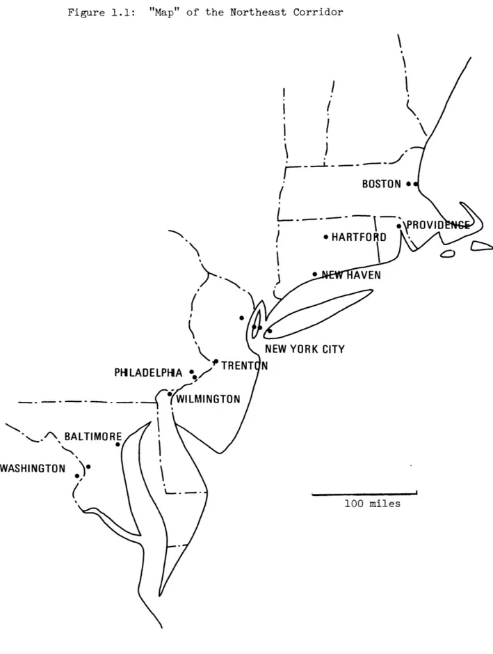
1.1 Introduction to the Northeast Corridor

The Northeast Corridor is the area between Washington, Philadelphia,

New York and Boston. Six other cities, Baltimore, Hartford, New Haven, Trenton, Providence, and Wilmington complete the list of major traffic centers.

Figure 1.1. is a map of the area. The corridor is interconnected by inter-state highways, passenger rail service, and either direct or indirect

commercial flights.

At present over 80% of the passenger traffic among these cities travels

by car. This is true even though the circuity of the roads and the delay of

gas and toll stops reduce the average speed of highway travel to 41.1 mph

"as the crow filies". Trains and buses, traveling at similar effective speeds, carry less than a tenth of the traffic. The remainder of the trips are made on aircraft, in spite of delays which stretch the sum of take off and landing times to an average of 35 minutes.

The performance of the current public modes of travel is deteriorating with increasing numbers of travelers. Two solutions have been proposed:

(1) improved rail transportation emphasizing the use of existing rights of

way along the back bone of the corridor and (2) improved air transportation using aircraft and facilities dedicated to short haul traffic.

Figure 1.1: "Map" of the Northeast Corridor BOSTON

\

/

HARTFORD

BALTIMORE

NEW YORK CITY

100 miles

-1.2 A Short Haul Air System

There are great advantages in getting the short haul aircraft out of the current airport traffic. Reduction of congestion at the major airports of the Corridor would reduce expensive delays in both long and short

aircraft flights. This would permit expansion of long haul air service. In addition the divorce of both vehicle and terminal from long haul operations can allow a short haul air system to serve what has become a mass transport market.

A new and separate short haul air system would include: (1) new

aircraft designed to reduce aircraft take off costs and to use inexpensive terminals, (2) multiple new metroports located for convenience and designed to reduce the cost and delay of boarding the aircraft, (3) an air traffic control environment that permits direct routing, minimal loitering times, and all weather operations without interfering with long haul traffic, and (4) a corporate structure which separates the short haul operations from long haul service.

This report will concern itself with items (1) and (2), aircraft and metroport considerations. Air traffic control is a relatively small part

of the system cost, and therefore has not influenced this discussion. A brief discussion of the air traffic control problems is presented in Appendix A. Institutional factors have been left to less technical discussions. This analysis assumes that metroports are financed by tax exempt bond issues and run without loss, and that the aircraft are managed

1.3 Possible Configurations of a Short Haul System

There are two major candidates for a new short haul air system based on the type of aircraft used. A STOL system offers the relatively low mileage costs of STOL aircraft at the expense of complication of terminal operations. A VTOL system offers more efficient terminals but higher cruise expense. Let us look first at the STOL system.

The set of 15 metroports in table 1.1 is a proposed STOL network. The terminal sites were selected on the basis of both access convenience and total cost. Each site has space for a single 2000' runway and is situated to reduce noise impact. These sites may not all be politically feasible. The expense of elevated city center metroports has forced the selection of existing airport sites for most operations. Initially, a downtown STOL system was studied, but was found prohibitively expensive.

The competition is offered by the corresponding 15 terminal VTOL system in Table 1.2.

In order to choose between these two systems one must consider

(1) community acceptance (noise, safety, etc.), (2) ease of implementation,

(3) overall system cost, (4) flexibility, (5) compatibility with the

current CTOL air system, (6) the changing importance of city center congestion, and (7) technical performance, i.e. the ability to attract sufficient numbers of travelers to operate without financial loss.

This report evaluates and compares technical performance only. The other six considerations are briefly discussed in the last chapter.

-Possible STOL Metroport Locations

New York City

Secaucus STOLport site La Guardia Flushing site

Over an interchange on route 287 in White Plains near Westchester

Logan Airport STOL strips (new) Hanscom Field STOL strips (new) Philadelphia

Over 30th Street Railroad Station (elevated)

Across Schuykill River from Conshocken, by an expressway Washington

Over Union station (elevated)

Washington National STOL strips (new)

Baltimore

Over Port Covington Rail Yard Hartford

Brainard Airfield STOL strips (new)

Trenton TTN

New Haven NHV

Mercer County Airport STOL strips (new)

New Haven Airport STOL strips (new) Providence

SPV Providence Airport STOL strips (new)

Wilmington

SWL New Castle Airport STOL strips (new)

SEC LGF WES Boston BOS HAN SPC SPW SUN WAS SBL HRD Table 1. 1

Possible VTOL Metroport Locations

New York City

Manhattan on West 30th Street docks

Manhattan on East River south of U.N. (not included in the

STOL comparison)

La Guardia Airport Newark Airport

Over North Station (downtown)

Intersection of route 128 and Mass Turnpike

Philadelphia

Over 30th Street station

Across Schuykill River from Conshocken

Washington

Over Union Station Washington National Baltimore

Over Port Covington rail yard Hartford

HRD Braina rd Airfield

Tranton

TTN Mercer County Airport New Haven

SNH Over Railyard near Connecticut Turnpike

Providence

SPV Over downtown trains Wilmington

SWL Over Cherry Island railyard

6 -JMW JME LGA EWK Boston JNS J28 SPC SPW SUN WAS SBL Table 1. 2

1.4. Report Structure

This project begins with a set of assumptions about component costs and ends with the selection of a system which is in some sense optimal. The development of time and cost structure for a V/STOL system is given in Chapter 2. Detailed development of individual numbers has been relegated to the appendices. Once the structure for assembling and comparing different systems is established, the system which can attract the greatest traffic without loosing money is found by what is basically a cut and try method. This is done in Chapters 3 and 4. The crude assumptions of the basic structuring are checked in Chapter 5 by exercising the chosen system in a more sophisticated network study. Chapter 6 summarizes the effort and reviews its limitations.

The reader may originally be surprised at the extensive discussion in Chapter 3 and 4 of what has just been described as a "cut and try" approach. In fact, the author has attempted to explore over a broad range the forms a V/STOL transportation system could take. The work in Chapter 3 is independent of demand, and merely defines the range of operating

conditions achievable by V/STOL systems. The concept of a three dimensional surface of possible operations is introduced.

It is only in Chapter 4 that a corresponding surface ,conveying information about the collective desires and values of the users of the system is introduced and by comparison of the surfaces, a "best" system is determined.

The purpose of this somewhat roundabout procedure is to arrive at the destination with some idea of where we have been.

2. METHODOLOGY FOR DEVELOPING THE PERFORMANCE OF V/STOL

2.1 Defining the Performance of an Air Transportation System

For the purposes of this study, the performance of a transportation system is measured by the total cost and total time with which it can serve a given size travel market without a loss. This performance depends not only on the type of system, STOL or VTOL, but also on internal adjustments of the system design. Changes in aircraft capacity, average frequency, number of terminals, and number of direct flights can adjust a single type of system over a wide range of cost and time. This chapter establishes the framework for these design options.

The total cost of a trip is the ticket price plus access (and egress) costs. The ticket price is the shared system cost composed of:

(1) a share of the cost of capital investment in terminals.

(2) a share of terminal operations and take off costs and

(3) a share of the aircraft mileage costs.

To this will be added the access and egress costs. The details of all costs will be explored in the next section.

The total time of a trip includes:

(1) the time spent in flight

(2) the time spent in boarding, taking off, and making intermediate stops

(3) a time associated with waiting for a convenient departure. This

time is related to the daily frequency.

and (4) access and egress times to and from the terminals of the system.

-2.2 The Structure of V/STOL Trip Costs 2.2.1. Sharing Method for Capital Costs

A major consideration in the design of a STOL or VTOL system is the

cost of the terminals. If the cost is too high, the system very quickly becomes overpriced. Capital investments are assumed to be made at the beginning of a system's life. Land is purchased and buildings are

constructed. Financing would normally be through local bond issues. The difficulty lies in allocating the costs in an equitable way. The simplest possibility is to repay interest and debt equally over a 20 year period like a home mortgage. Each boarding passenger pays an equal share of the annuity. This was the method followed.

2.2 Development of Capital Costs

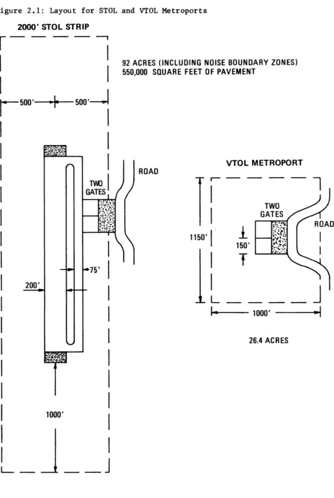
Good metroport design can save considerable expense and reduce transit times. The great advantage of a V/STOL system is the low cost of the

airports. Suggested metroports have shown tremendous variations in cost and convenience. In view of the magnitude of cost variations, and the importance of the metroport performance to the system, the design used in this study was chosen with careful consideration.

The gate positions were chosen from design #8 by Allen and Simpson (Reference 1). This design provides a swift boarding procedure at a minimum of capital or operating expense. The cost of a gate position designed to accommodate eighty seat helicopters was estimated at $2.02 million. Two

thirds of the cost is proportional to vehicle size.

STOL Runways and taxiways were assumed to cost $0.667 million

Figure 2.1: Layout for STOL and VTOL Metroports

92 ACRES (INCLUDING NOISE BOUNDARY ZONES)

550,000 SQUARE FEET OF PAVEMENT

I

IA

VTOL METROPORT

H-500'

-A-0-I

GATE

I

200'I

I

1000'

F

- -

-1

I

T

L

-1150'

$.5 million was included to represent the cost of half a mile of

elevated and half a mile of ground level roadway for access.

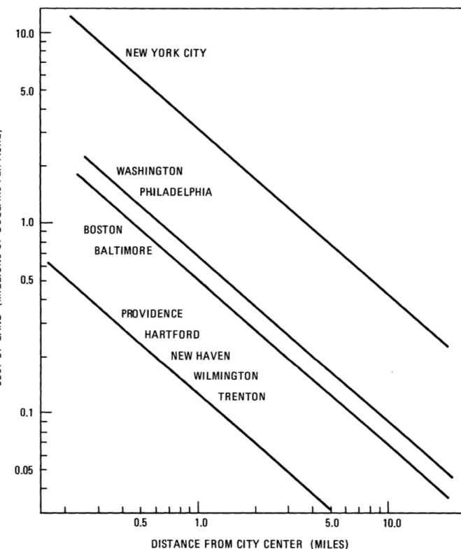
The layout for the STOL and VTOL ports is illustrated in figure 2.1. Borderland around each landing site must be purchased because other use

is impossible for noise reasons. In cases where the STOL port is located on an existing airport, the land is free. Otherwise the land cost is derived from figure 2.2.

The minimum number of gate positions is two. If the traffic warranted it, more gates were added at cost.

Following these guidelines, the total ground system investment is $252 million for VTOL and $406 million for STOL (see tables 2.1 and 2.2). If financed by 20 year 4.5% bonds these figures become $19.4 and $31.2 million per year respectively. This reduces to $2.66 and $4.28 per boarding if there are 20,000 passengers a day for the total system.

2.2.3. Terminal Maintenance

Maintenance costs for the terminal buildings are estimated a $1.68/ft2/year (reference 13 in 1970 dollars) or $38,400/gate/year. Maintenance is shared just like the capital costs. The annual total is $1.15 million per year for

30 gate positions. This is $0.16 per passenger for 20,000 passengers per

day.

2.2.4. Processing Costs

An efficient short haul system will need an automated ticketing system to avoid labor costs. Credit card holders will be able to write their own tickets using machines at the airport. Presumably reservations and

Cost of VTOL Metroports Metroport Name JMW JME LGA EWK JNS

J28

SPC

SPW

SWL

SPV

$

4.54

4.54

4.54

4.54

4.54

4.54

4.54

4.54

4.54

4.54

4.54

4.54

4.54

74

26

79

35

65

1) All costs in millions

2) The cost of unimproved land is used to represent the cost of sharing

improved land such as at North Station in Boston

3) The cost of 15 terminals is 15/16 of the cost of 16 terminals

- 12 -Total Cost $ 48.54

48.54

4.54

4.54

15.64

4.54

40.34

4.54

4.54

6.34

6.14

.67

.56

.136

$ 44.0

17.7

35.8

1.8

.6

Table 2.2 Cost of STOL Metroports

cost of

Metroport roadrunway, Percent of

Name Cost/acre Land Cost and 2 gates Total Cost Metropolitan Market

SEC $ 1.05 $ 96.6 $ 5.21 $ 101.81 68% LGF x 0 5.21 5.21 20 WES .3 26.6 11.21 37.81 12 BOS x 0 5.21 5.21 86 HAN x 0 5.21 5.21 14 SPC .67 61.8 11.21 73.01 79 SPW .072 6.6 5.21 11.81 21 SUN .56 51.6 11.21 62.81 35 WAS x 0 5.21 5.21 65 SBL .064 58.9 11.21 70.11 100 HRD x 0 5.21 5.21 100 TTN x 0 5.21 5.21 100 NHV x 0 5.21 5.21 100 SPV x 0 5.21 5.21 100 SWL x 0 5.21 5.21 100 TOTAL: $ 406.25 Notes

1) All costs in millions

2) The cost of unimproved land is used to represent the cost of sharing improved land such as at 30th street station in Philadelphia

Figure 2.2: Cost of Unimproved Land in the Northeast Corridor

10.0

NEW YORK CITY

5.0 WASHINGTON c-PKILADELPHIA Co 1.0 1.0 BOSTON U--D BALTIMORE W M 0.5 PROVIDENCE HARTFORD U-0 _{NEW HAVEN} I-WILMINGTON TRENTON 0.1 0.05 0.5 1.0 5.0 10.0

DISTANCE FROM CITY CENTER (MILES)

Source: Eastman, reference 3

-2.2.5. Income from Parking

A significant percentage of air terminal operations is supported by income from nearby parking garages. There is no reason why garages

located on floors below the boarding areas can not contribute to V/STOL overheads.

Roughly 44% of the passengers come or go by car. (See appendix C) One quarter of these park for two days at $3.00 per day. A parking place costs $4,800 in capital costs or $1.00 per day. Labor costs are estimated at $0.25 per day per car. Assembling all this, the net income is $1.75 per day or $0.39 per boarding per day. This contributes to the support of the terminal.

2.2.6. Direct Operating Costs of the Aircraft

Direct Operating Cost (DOC) is usually half the ticket price. In a STOL or VTOL system, DOC's are expected to be higher since the aircraft is compromised to allow lower indirect operating costs (IOC's) and convenient access. This trend is balanced by the reduced take off and maneuver cost experienced by these aircraft. As a result DOC remains near half of the ticket price for short trips, but is higher at longer ranges.

Operating costs for both the helicopter and the STOL aircraft used in this study were derived from vehicles designed as part of an ongoing effort at the FTL. A 60% load factor was assumed for conversion to ticket costs. The results used in this report are discussed in appendix B. The conclusions are presented here.

It was found that the DOC of STOL and VTOL aircraft could be simply described as a combination of a take off and maneuver cost and a cost per

the seating capacity. As a result it costs on the order of $1.00 per take off and $.02 per mile for each aircraft seat. These figures go up consider-ably for smaller aircraft. Using a load factor of 60%, each passenger would be charged roughly $2.00 per take off plus $.04 per mile for his trip.

Variations depend on aircraft size and type. Large aircraft are cheaper. VTOL aircraft cost less per take off, but more per mile. In addition, multistop operations cause a greater burden of take off costs.

2.2.7. Stewards

Stewards (male or female) are necessary for safety and boarding, even though no inflight service is necessary. One steward for every forty passengers was assigned to each aircraft. $8.40 per hour was charged against stewards during boarding, takeoff, maneuver, and flight times. These costs, although technically indirect operating costs, were added to the aircraft DOC because they accrue in exactly the same manner.

2.2.8. Aircraft Handling Costs

Short haul aircraft will not be fueled or inspected at every stop. To cover these intermittent servicings, a charge of $6 per landing I is

added to the aircraft DOC. Ground handling costs,like stewards' salaries, vary directly with aircraft activity.

Reference 8 suggests $10.70 if refueled at every stop.

-2.2.9 Operating Overheads

Overhead comes from general and administrative expenses and includes before taxes profits. Since the cost of managing is proportional to

the size of operations, overhead was estimated to be a percentage of the total ticket price. Simple operations are assumed to cost 22% of the ticket price.

2.2.10 Total Ticket Price, an example

A short haul ticket cost can be assembled from the several costs

listed above. For example

$ 3.00 - contribution to terminal capital costs

.17 - terminal maintenance

-.39 - income from parking concession

2.00 - ticketing costs

2.41 - aircraft DOC, handling IOC, steward IOC for the take off and maneuver

4.13 - Cruise costs DOC and steward 1OC for 200 miles 3.18 - 22% G & A and Profits

$14.50 - AIRLINE TOTAL

1.16 - 8% ticket tax (equaling ATC expenses)

$15.66 - Ticket Price

2.2.11 Access and Egress Costs

Demand models relate the volume attracted by a new mode to the total perceived cost of travel on that mode. This cost of travel is the sum of

ticket price and access and egress costs. A new V/STOL system can spend

more on its terminals and charge more for its services if it can reduce the average access costs enough.

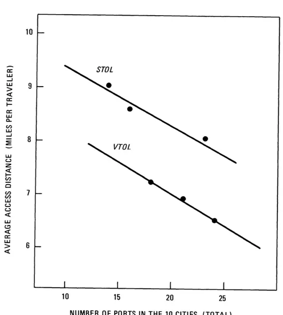
Access costs are developed for all modes in appendix C. Figure

2.3 illustrates the results of a study of possible terminal locations

in the Northeast corridor. (Appendix D contains discussion of the location methodology.) The average access distance for all potential passengers in the ten metropolitan areas is dependent upon the total number of metroports in the corridor. More metroports offer easier access. Failure to locate STOL sites near the city center puts the STOL system at a slight disadvantage.

The sum of access and egress costs is typically near $4.00 for a V/STOL trip. The cost performance of the V/STOL system would be the ticket price plus the access costs or $15.66 + $4.00 = $19.66 for

the 200 mile trip in the preceding example.

-Figure 2.3: Average Access Distance to V/STOL Terminal as a Function of the number of-Metroports in the Corridor

(points developed from case studies)

NUMBER OF PORTS IN THE 10 CITIES (TOTAL) STOL

81

I II I

I

I

2.3 The Structure of V/STOL Trip Times

The trip cost of a V/STOL system is only half of the performance picture. The other predictable index of performance is the total trip time. This involves not only the speed but also the convenience of the scheduled departures.

Viewing a trip through the traveler's eyes the successive steps are: access, boarding, flight time, disembarking, and egress. It is in this order that the times are discussed.

Access times are dependent on access distance. Once again the discussion of appendix C and the data of figure 2.3 apply. Access time is lower for VTOL than STOL operations because of the more convenient metroport locations. As before, increasing the number of terminals

can cut access time for either system. An average access time might be 35 minutes.

Boarding through the gate positions should be fast. An average of seven minutes is assumed, although faster processing can easily be imagined with this particularly direct design.

Flight time is composed of takeoff and maneuver time plus time spent in cruise. V/STOL vehicles achieve flight conditions in very little time. The STOL aircraft spend about 10 minutes in takeoff and landing maneuvers.1 VTOL aircraft do without taxiing and cut this

figure in half. On the other hand, cruise speeds are quite low. The

STOL aircraft of our design cruise near 300 mph. The helicopters

cruise even slower, 240 mph. Thus a 200 mile journey could take from

lThis is the design performance as presented in Appendix B.

-40 minutes to an hour. Later designs can achieve higher speeds. Additional flight time would be experienced by a traveler if he is on a multistop trip. An intermediate landing would add a second increment of maneuver time plus an additional seven or eight minutes of turn around time. The 15 minute penalty is paid only in

multi-stop flight operations. Multistop operations are used if the

daily frequency would be too low (4 to 7 flights per day) using

single load flights.

Upon arrival at his destination the passenger should be able to disembark in three minutes and achieve his final destination with

roughly another 35 minutes of egress time.

A tally of the travel times above might look like this for the

typical 200 mile trip:

35 min. access time (average) 10 min. boarding plus disembarking

5 min. aircraft maneuver time

60 min. flight time (2oo miles)

12 min. intermediate stop maneuver and turnaround

35 min. egress time (average)

Total 2 hours 37 minutes

The last influence on the time is the frequency of service, i.e., the convenience of departure times. An artificial index of this con-venience was chosen. Half the average headway was added to the total time to give the time performance of V/STOL service. Thus for 6

flights in a 16 hour day the timeliness delay is 1/2 - (16 + 6) = 1.33

hours. If two demands can be combined into a single route, twice the

.67 hours. Adding this to the total travel time produces a total

trip time of 3 hours 17 minutes.

The data of the preceding sections is repeated in Appendix I., Standard Conditions for 1985 QVTOL studies.

-3.0 THE PERFORMANCE OF V/STOL TRANSPORTATION SYSTEM

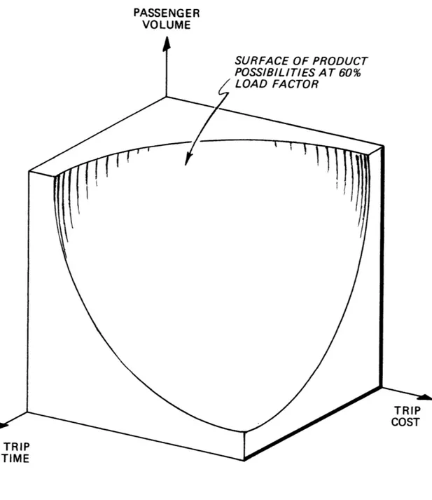
3.1 The Concept of a Product Possibilities Function

Figure 3.1 illustrates the three dimensional surface which forms the product possibilities I function for V/STOL transportation in the Northeast Corridor. It is a surface of "best" system performance measured by total trip time and cost. Notice as passenger volume is increased that average total trip time can be reduced due to increased frequency of service. Average total trip cost is also reduced as the cost of terminals is spread over more passengers.

Each point on the surface is a possible operating condition of some VTOL or STOL system. The surface was defined by cut and try. Each point on

the surface is defined by a specific aircraf-t size and type and a specific set of terminals. Operating the same system at a traffic volume below that

indicated by the surface will result in a loss. Operating at volumes above a given point on the surface, but still at the same trip time and cost, will produce a profit if the assumed load factor (60%) is maintained. 2

The surface does not portray the performance of any single- system. Each part of the surface is defined by the specific system which can perform "best" in that region. Best performance means carrying the minimum traffic volume at the stated cost and time without a loss. Thus the surface is a combination of STOL and VTOL systems both large and small. The aircraft

type and size varies over the surface. The number of gates at each terminal

Although functionally similar to the economic concept of production

possibilities, this new term refers to a different phenomenon. See Appendix E. There is no reason why the concept could not be extended to more dimensions

Figure 3.1: Product Possibilities Function for a V/STOL Transportation System PASSENGER VOLUME SURFACE OF PRODUCT POSSIBIL ITIES AT 60% LOAD FACTOR - 24

-inm milw4 i I 1 i

and indeed the number of terminals can vary also. A minimum of 2 gates per terminal and 15 terminals was enforced.

The remainder of this section will be devoted to discovering which systems dominate the different areas on the surface. To do this

horizontal cuts through the surface are made and the set of cost-time tradeoffs available at the constant passenger volume is graphed. These curves are called "isoquants". In order to fix specific numbers to the cost and time,a representative route was chosen2 at 200 miles. The volume on the route was such that 274 round-trip passengers a day represented a total of 20,000 trips on all the routes in the V/STOL system for the whole Northeast Corridor.

3.2 Product Possibilities Function for VTOL and STOL

3.2.1 VTOL Performance

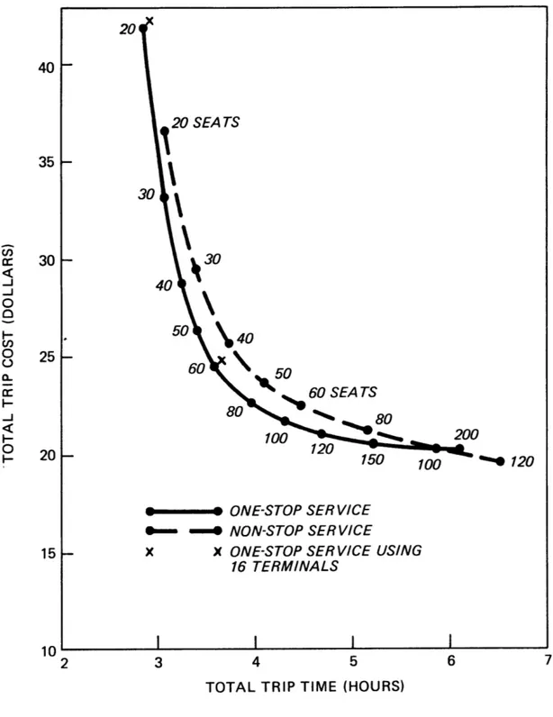
Figure 3.2 is a graph of the performance choices for a helicopter based system carrying 20,000 passengers per day. Each point on the graph was developed using the methodology of chapter 2. The set of fifteen

terminals was used to evaluate fixed costs. A specific volume of traffic

was postulated and a vehicle size was assumed.- The resulting unit costs and frequency of service at 60% load factor produced the points on the graph.

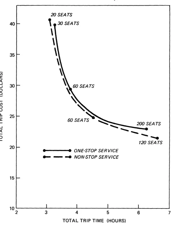
The area of the curve closest to the origin is of the greatest interest since this is close to present airline services. In this area one stop service by small to intermediate size aircraft performs best. At extremely low costs (and high times) nonstop service by larger aircraft is better. Also at very low times and high costs one stop service using very

small aircraft is competitive.

The two small x's on figure 3.2 illustrate the effect of adding another terminal. The x's mark the system operation if a second Manhatten

terminal is built on the east side. Both trip cost and trip time are worse. The unit cost goes up because the additional capital costs must be defrayed. Trip time goes up because the addition of eight new markets (from splitting up old markets) has reduced the market size on each route, thus reducing the daily frequency. The savings in access time and cost are not enough to compensate under stated assumptions. 1 The minimum number of terminals

(arbitrarily 15) was best for all V/STOL systems studied.

1 If access costs are more important, or if they are larger due to

congestion, these conclusions can be reversed.

-Figure 3.2: Isoquant for VTOL (helicopter) at 20,000 trips per day representative route length of 200 mi.

fifteen terminal network represented

TOTAL TRIP TIME (HOURS)

40

t-35

}-30

F-25

60 \ *06 50 60 SE A TS

80

_{%% *-w80}

100

''-,

200

ONE-STOP SER VICE

- NON-STOP SER VICE

x X ONE-STOP SERVICE USING

16 TERMINALS

3.2.29 STOL Performance

Figure 3.3 is the same drawing for the STOL system. Here the nonstop operations are everywhere better than multistop routings. This

is because of the higher maneuver costs for STOL. Once again moderate size aircraft dominate the region near the origin.

3.2.3. STOL and VTOL compared

Figure 3.4 is an altogether different look at the 3-dimensional supply function. Here a slice has been made at an angle to both cost and time axes. The plane is determined by the point cost = $25, time = 3.5

hours, volume = 20,000 passengers and the line forming the volume axis. This plot shows that for all reasonable volumes VTOL service is better than STOL

service. STOL is better only for extremely low time and extremely high cost operations at high volumes. Almost all of the surface is dominated by

helicopter based systems.

Four general areas (A,B,C, and D) are suggested on the product possibilities function redrawn in figure 3.5. Except for extreme values of time or cost, the area is dominated by one-stop helicopter service using 40 to 80 seat aircraft.

If passenger volumes are high, and trip time is not as important as cost, a nonstop helicopter service is indicated using large vehicles.

If passenger volumes are high and times is of essence, a high frequecy helicopter system using nonstops service is cheapest.

If passenger volume is extremely high and time is extremely impor-tant, a STOL system is best. At high volumes STOL port costs are low since they are shared among many people. In addition, large STOL aircraft designs tend to be relatively cheaper and faster than larger helicopters. Nonstop

-service is indicated.

If passenger volumes are low or moderate and if there is a balancing of time and cost priorities, a service using a 40 to 80 seat helicopter is best. On longer flights the passengers would experience an intermediate

stop.

Sneaking a look ahead, the demand forces us to look at the area inside line NEM. In this region a viable VTOL system can exist because the demand is available. Another way of looking at is that a less than 60% load factor is economic. We now turn our attention to forecasting the demand for an average market in the Northeast Corridor in order to pick the appropriate VTOL or STOL system.

Figure 3.3: Isoquant for STOL service at 20,000 trips per day representative route length of 200 mi.

fifteen terminal network represented

TOTAL TRIP TIME (HOURS)

- 30

-40

35

25|

-~

60 SEA TS

60 SEA TS

200 SEA TS

- ONE-STOP SER VICE

- - - NON-STOP SERVICE

-20

15

Figure 3.4: Vertical Slice through Product Possibilities Function for V/STOL Service

60t- 50140 -30 1-20 --- ONE-STOP VTOL -- NON-STOP STOL

sq.

K,

DEMAND

TOTAL TRIP TIME (HOURS)

I I 1 1

20 30 40 50

TOTAL TRIP COST (DOLLARS)

Figure 3.5: Intersection of Demand Surface on V/STOL Product Possibilities Function

REGION A:

REGION B :

REGION C :

NON-STOP VTOL, LARGE AIRCRAFT NON-STOP STOL

NON-STOP VTOL, SMALL AIRCRAFT REGION D: ONE-STOP VTOL

POINT E : VOLUME = 23,500 TRIPS PER DAY

THE LINE N E M IS THE INTERSECTION OF THE

DEMAND SURFACE FOR SOME YEAR ON THE

PRODUCT POSSIBILITIES FUNCTION

-1 IIN1i11 1fl i ll

4.0 THE MARKET FOR V/STOL TRANSPORTATION

4.1 Concept of Demand

The last two figures have included "demand" curves along with the product possibilities function for V/STOL transportation. These demand curves are developed from a demand survace that has much the same shape used in figure 3.1 to illustrate the product possibilities function. The demand surface reflects the maximum number of passengers that would be attracted from the existing air, rail, and highway modes to a new system. At each time and cost a specific volume of travelers prefers the new mode. As time and cost are reduced, these volume increases.

The demand surface is developed using a modal split demand model which compares the performance of a new mode to the existing performances to estimate the percentage of the traffic that will be attracted.

Any individual point on the demand surface marks the largest possible volume that could be attracted by a mode offering the stated performance. All the points below the demand surface represent possible operating conditions for a system offering this performance.

Constant volume "indifference" curves for typical demand in 1978 (as &rived from Appendix G)are plotted in figure 4.1. The convexity of the

demand surface is slightly less than that of the supply function.

4.2 Intersection of Demand and Product Possibilities

Figure 4.2 is a horizontal (constant volume) cut through both the product possibilities and demand surfaces. The curves are called an isoquant and an indifference curve respectively. The shaded area between

Figure 4.1: Total Demand for V/STOL Transport in the Northeast Corridor

in 1978 (indifference curves)

2 3 4 5 6 7

TOTAL TRIP TIME (HOURS)

NOTE: CURVES REPRESENT CONDITIONS WHICH WILL ATTRACT THE STATED DAILY TOTAL VOLUME

OF TRIPS.

-Figure 4.2: Product Possibilities and Demand for V/STOL Travel in 1978

15,000 trips per day

representative route length of 200 mi.

3 4 5 6 TOTALTRIPTIME (HOURS) 30 25 20

10

the two curves represents possible operating conditions. The points

within the area are feasible from both a profit and a marketing viewpoint. Figure 4.3 is the same graph, plotted at a higher volume. The isoquant for the STOL system has been included to show that there is no solution at this volume. For VTOL the shaded area is smaller, however another 5,000 travelers find the new service a desirable convenience.

As the volume level is increased points M and N more closer together until they form a single point. The demand and product curves are tangent at 23,500 passengers a day. This is a $24.00 trip with a time of 3.4 hours. A 60 seat helicopter flying multistop services is indicated.

Figure 3.5 illustrates in three dimensions the line formed by the intersection of the demand surface with the product possibilities. This line corresponds to the points M and N. Point E is the maximum possible equilibrium volume. Above this level no V/STOL system can match the existing demand without a loss when operating at 60% load factor.

The intersection point, E, is a characteristic of the market and system interactions. This point has been chosen as the statistic with which systems will be compared. Other intersecting points also could be compared. At higher costs, slower time, and lower volumes there is a point where distance in the direction of the cost axis between the product possibilities function and the demand surface is the greatest. This is the point of maximum profit per passenger. Near it are points of maximum profit as a percent of ticket price and as a percent of capital investments. If the ticket price can be raised enough, it benefits private enterprise to operate at higher frequencies and with smaller aircraft than exist at the maximum volume point.

-Figure 4.3: Product Possibilities and Demand for V/STOL in 1978 20,000 trips per day

representative trip length of 200 mi.

40|-r--VTOL

35

30

1-

251-N

20

15

I-3

4

5

6

TOTAL TRIP TIME (HOURS)

The maximum volume point has been selected as a basis for measuring the system both because it is the clearest unique point and because it is the point usually considered in system planning studies. In any case it is a good representative of system operations.

4.3 Redefinition of the Vehicle for a Mature System

The next sections explore the behavior of the system near the maximum volume intersection. Before doing this, however, the ground rules

are going to change: 1985 volume levels 1 are going to be examined. In addition a new set of helicopters designed at the Flight Transportation Laboratory will be used. These vehicles were particularly designed to be quiet -- 82.5 pndb at 500 feet in take off and 70 pndb on the ground

during cruise. The DOC's are presented in Appendex B. Quiet operating conditions are typical of acceptable new urban operations and would have been used for the STOL/VTOL comparison if appropriate STOL designs had been

available. This new system is called a QVTOL system.

Using these ground rules changes the location of the maximum volume intersection point, point E on figure 3.5 The new intersection of product possibilities and demand is at 35,000 passengers per day. A 60 seat

helicopter is called foroperating one stop routes.

Figure 4.5 illustrates the intersection of 1985 demand and QVTOL product possibilities at a volume of 35,000 travelers. The 80 seat vehicle is nearly as effective as a 60 seat vehicle.

1 1985 demands are 35% above 1978 demands. The indifference curves for the

demand surface are presented in figure 4.4.

-Figure 4.4: 1985 Demand

DEMAND LEVELS IN THOUSANDS/DAY

2 3 4 5 6 7

TOTAL TRIP TIME (HOURS)

Figure 4.5: Intersection of 1985 demand surface and QVTOL product possibilities function at volume*35,000 trips

2 3 4 5 6 7

TOTAL TRIP TIME (HOURS)

-4.4

The intersection of product possibilities and demand is a

very shallow one, as can be seen in figure

4.6.

4.6

vertical slice through the product possibilities and demand surfaces at the angle cutting through the optimum point. Any small

perturba-tion of the cost of QVTOL service would result in a drastic change in the maximum volume that could be carried. Similarly any change

in the demand function creates equally dramatic shifts in volume. It is interesting to note that while the maximum volume can change quite radically, the operating conditions are nearly the same throughout. The minimum number of terminals, 16 for the QVTOL study, is still desirable, and a 60 seat vehicle can serve the market

adequately over a wide range.

Figure 4.7 displays the product possibilities function at several volume levels. Between 5,000 and 20,000 travelers per day the system is barely creeping along. Terminals are severely

under-utilized. Multistop service would be used on most routes. Above

50,000 travelers the terminals have costed themselves out and nonstop

services have been implemented. Some savings result from the very small advantages of using aircraft over 80 seats capacity. Additional gate positions and eventually additional terminals allow the system to expand to carry quite large volumes before congestion sets in to

Figure 4.6: Vertical Slice through Product Possibilities Function for QVTOL Service

2 3 4 5 6 7

TOTAL TRIP TIME (HOURS)

I I I

TOTAL TRIP COST (DOLLARS)

-Figure 4.7: QVTOL Product Possibilities Function at various volumes

2

3

4

5

6

7

TOTAL TRIP TIME (HOURS)

4.5 Variation of QVTOL System Parameters 4.5.1 Variation of QVTOL Performance: DOC

In Figure 4.8 the performance of a system employing aircraft

with DOC inflated by 25% is compared to the standard QVTOL performance.1

The effect produces a marked change in the trip costs. The maximum

equilibrium volume drops from 35,000 to 26,000. Most of this drop comes from the penalties of cruise costs. A 25% increase in takeoff costs alone has a very small effect since takeoff costs are relatively small originally.

4.5.2

Variation

In Figure

4.9

has been altered from what is available through efficient terminal

design and operation. Costs at airline levels are even more detrimental to operation than increased DOC. The maximum volume is only 23,000 trips per day. This is a good argument for separating a new short haul

system from current airline operations. Spartan processing operations

must be insured.

4.5.3 Variation of QVTOL performance: Changes in Capital costs

Once VTOL daily volumes exceed 20,000 trips, the importance of the capital investment costs is reduced dramatically. This is one advantage of VTOL systems, the "fixed" capital costs are the lowest for any high performance system. STOL systems, the next best, have

1

Both costs and times were made 25% worse.

-Figure 4.8: Effect of DOC on QVTOL Isoquant; volume=30,000 trips

3 4 5 6 7

TOTAL TRIP TIME (HRS)

10 ' 2

Figure 4.9: Effect

40

-35

of processing costs

QVTOL isoquant at volume=30,000 trips per day

2

3

4

5

6

7

TOTAL TRIP TIME (HOURS)

-nearly twice the capital costs. For the 1980 - 1990 framework, and until tilt rotor vehicles make both STOL and helicopters obsolete, the traffic in the Northeast Corridor is best carried by the helicopter system. A change in the capital costs of t 25% is barely noticeable, changing the

maximum volume point by only - 4%.

4.5.4 Variation of QVTOL Performance: 1980, 1990 demands

The demand for travel does not affect the performance function for V/STOL systems. Only the demand surface changes. This simple analysis assumed the 1990 demand was 18% greater than 1985 demand.

This can be done merely by changing the volume scale on the demand

surface. The shape is unaltered.

Table 4.1 lists the demand levels and the performance of a

QVTOL system for the years 1978 - 1990. The table highlights two very important phenomena. First, a 60 seat vehicle is optimal over

a wide range of volumes. And second, as volumes increase, terminal

activity remains constant because fewer multistop flights are flown. Thus a system built for 1978 is still optimal in 1990 even though travel has doubled!

4.5.5 Variation of QVTOL Performance: Comparison with a Tilt Rotor

By 1985 it is entirely possible that a tilt rotor VTOL vehicle

would be manufactured to take the place of the conventional helicopter. Information from tilt rotor designs performed at the Flight

method is crude, especially since the tilt rotor tends to be harder to quiet than the helicopter, but it was the only avenue available. The result was a vehicle with the following parameters:

Cruise speed is 400 mph

Cruise DOC is $.585 per aircraft plus $.00498 per seat Takeoff DOC is $39.50 per aircraft plus $.521 per seat Takeoff and maneuvre time is .054 hrs.

The tilt rotor can use VTOL terminals, but has a cruise speed and cost that approaches the performance of advanced STOL aircraft. A sacrifice in takeoff costs is made compared to helicopters. The performance of the quiet tilt rotor is compared to the quiet helicopter (QVTOL) system in Figure 4.10. Clearly the saving in cruise time and cost increases the capabilities of the system considerably. Indeed the maximum volume point is at 51,000 trips per day. The optimal vehicle size is still 60 seats, in spite of an altered cost structure for the DOC.

Table 4.2 compares the performance of the quiet tilt rotor with the quiet helicopter system. Tilt rotor vehicles offer essentially the same service at reduced cost. A 60 seat tilt rotor is used nonstop to replace a 60 seat helicopter operating multistop routes.

-48-System Sizes for QVTOL at Maximum Volume Optimum

1978 1 1980 1985 1990

Total Demand levels2 (all modes)

QVTOL Performance

(optimal volume) Number of Vehicles Used

(2300 hrs per year)

Size

( (number of seats) Average daily landings

per terminal Ticket Cost

(1970 dollars)

Daily one way frequency on representation route 160,000 176,000 216,000 256,000 20,000 82 60 71 $21.3 7.0 25,000 100 60 86 $20.6 8.5 35,000 44-45,000 139 175 or 105 60 60 or 100 90 76 - 94 $18.2 8.9 $16.8-17.5 7.5- 9.3

1_{Actually these aircraft could not be in service before 1980.}

2_{Demand levels are indicative of relative market sizes only. For}

conversion to actual daily trips expected in the corridor, see discussion in appendix F.

MW MMMIN16

PAGES (S) MISSING FROM ORIGINAL

Figure 4.10: Comparison of Quieted Tilt Rotor System with Quiet Helicopter isoquant at 35,000 trips per day

3 4 5 6 7

TOTAL TRIP TIME (HOURS)

1

2

System Sizes for QVTOL and Quieted Tilt Rotor at

Maximum Volume Optimum

1985

Total Demand level (all modes)

Performance

(at optimal Volume) Number of Vehicles Used

(2300 hrs per year)

Size

(number of seats) Average daily landings

per terminal Ticket Cost (1970 dollars) Frequency on representa-tive route 216,000 QVTOL TILT-ROTOR 35,000 51,000 139 168

60

60

60

5.0 CASE STUDY OF 1985 QVTOL

5.1 Introduction to the Case Study

Up to this point a simple market model employing demand and

product surfaces has been used to predict the aggregate V/STOL activity that could exist in the N6rtheast Corridor. The model has suggested that a 16 terminal VTOL system using 60 seat vehicles would work. To test this prediction a market by market study of the corridor was made. This study involved creating and scheduling a network to serve the specific intercity markets in the corridor. The tool that

allowed this to be done is called FA-4.

FA-4 is a fleet assignment model created at the Flight

Transportation Laboratory (ref. 17). This model assigns aircraft to

specific routes in such a way that the daily frequency for each market is built up to attract passengers. FA-4 will continue to schedule flights as long as the income from the additional passengers attracted to the service covers the expense.

The procedure in FA-4 is economically different from the processes used in the product possibilities and demand study above. In the product possibilities function the ticket price was built up from the costs incurred. During this process the capital (i.e. long term) costs of the terminals was shared among the daily passengers.

In FA-4 the ticket price (or price structure, for each market has a different ticket price) is fixed. The model attempts to schedule

to maximize profits -- i.e. operate below the maximum volume at a point where the distance between demand and product possibilities surfaces is largel, and 2) it will not include the capital costs. This study of the individual markets can only confirm that at the given ticket price, capital costs can be recovered from excess

oper-ating profits.

In practice the information available from an FA-4 case study is more than just a check of a possible operating point of the market model. It is possible to consider a mixed fleet of aircraft. FA-4 can decide to use a small and expensive aircraft in order to get the frequency up in a particular market. Alterna-tively by proper route selection several services can be combined on a single flight and a larger aircraft employed. FA-4 can

answer two questions that the market model analyses cannot: 1) what

would happen if several different aircraft were simultaneously

avail-able to the system? and 2) what route patterns develop?2

Thus the purposes of the case study are threefold:

1) to check predictions of the product possibilities function

analysis by a study of individual markets, 2) to examine the attractiveness of a mixed fleet,

3) to observe developed route patterns

lStrictly speaking the FA-4 solution is interested in the cost

distance multiplied by the volume. The distance is between the pro-duct possibilities surface without capital costs and the demand surface at the established ticket price.

2

The conclusion in favor of multistop routes in the market model hints at the answer to this already.

-5.2 Performance as Defined in the Market Model

In Chapter 4 the product possibilities function was studied in the neighborhood of the maximum volume optimum. This point defined the largest volume of traffic that could be carried by any VTOL system without a loss. In 1985 this point was defined at 34,610 passengers per day carried by 60

seat helicopters. It is this point on the product possibilities function that will be tested in the case study.

A glance at figure 5.1 will reveal that most of the formulations

used in this market model are also used in the FA-4 system analysis. The IOC's that were used to build up the ticket cost are used as marginal

operating costs in FA-4. The DOC's used to describe the aircraft operations are also considered marginal expenses in the system analysis. Only the capital costs do not enter into the FA-4. If the optimum volume point in the market model is valid, the case study will have a total excess of ticket income over operating costs that will cover the fixed costs.

The work that went into evaluating the product possibilities function must be repeated for each city pair in the corridor for the case study. In the case study the whole network of markets, small and large, long and short, is examined. This means a specific distance, access, competition, and demands are necessary.

5.3 The Demand in each Market

The demand for VTOL service in each market is qualitatively illustrated in Figure G.1 Appendix G. This figure suggests that each additional daily service attracts progressively fewer passengers than the

modes' costs are the specific access and ticket costs for that city pair. The time is also the specific trip and access time by city. The line haul costs and times used the distance formulae of figure H.l. The frequency for the competitive modes is fixed. For the VTOL mode, frequency is varied to produce the demand curve.

The total demand for travel between any two cities is established from historical data. Table 5.1 lists the demands in 1978 for each city pair in the corridor. The 1985 demands are 35% higher.

This demand is splintered among the metroports in each city. Thus the New York - Washington market is split into eight separate markets among the six ports. Each port is treated as if it were a separate city.

For example consider the Manhattan west (JMW) and Washington Union Station (SUN) sites. JMW is closest to 25% of the New York trip origins.

SUN is best for 75% of Washington traffic. Thus the JMW-SUN demand is 19% (25% of 75%) of the New York-Washington demand.

1 The point of inflexion must be eliminated for successful _{solution. It can} be shown that the solution cannot be in the lower region for any single route.

-Figure 5.1: Data Flow Between Market Model and FA-4 flight schedules passenger traffic aircraft usage route selection UNINININNIOW