Life-cycle cost equations

Publisher’s version / Version de l'éditeur:

Vous avez des questions? Nous pouvons vous aider. Pour communiquer directement avec un auteur, consultez la première page de la revue dans laquelle son article a été publié afin de trouver ses coordonnées. Si vous n’arrivez pas à les repérer, communiquez avec nous à [email protected].

Questions? Contact the NRC Publications Archive team at

[email protected]. If you wish to email the authors directly, please see the first page of the publication for their contact information.

https://publications-cnrc.canada.ca/fra/droits

L’accès à ce site Web et l’utilisation de son contenu sont assujettis aux conditions présentées dans le site LISEZ CES CONDITIONS ATTENTIVEMENT AVANT D’UTILISER CE SITE WEB.

Building Research Note, 1979-09

READ THESE TERMS AND CONDITIONS CAREFULLY BEFORE USING THIS WEBSITE. https://nrc-publications.canada.ca/eng/copyright

NRC Publications Archive Record / Notice des Archives des publications du CNRC :

https://nrc-publications.canada.ca/eng/view/object/?id=8c3c216b-adb3-4ff9-8f1b-c24dd654c94b https://publications-cnrc.canada.ca/fra/voir/objet/?id=8c3c216b-adb3-4ff9-8f1b-c24dd654c94b

NRC Publications Archive

Archives des publications du CNRC

This publication could be one of several versions: author’s original, accepted manuscript or the publisher’s version. / La version de cette publication peut être l’une des suivantes : la version prépublication de l’auteur, la version acceptée du manuscrit ou la version de l’éditeur.

For the publisher’s version, please access the DOI link below./ Pour consulter la version de l’éditeur, utilisez le lien DOI ci-dessous.

https://doi.org/10.4224/40000563

Access and use of this website and the material on it are subject to the Terms and Conditions set forth at

Life-cycle cost equations

Ser

THI

B92

LIFE-CYCLE

COST EQUATIONS

by

R.K. Beach

INTRODUCTION

There is a growing concern about the c o n s e r v a t i o n and economical usc af natural resources, w i t h the ever increasing prices on one hand and thc possibility of shortages in supply en the other. It is important, t h e r e f o r c , t h a t architects, engineers, contractors, owners, and governments have a

clear understanding of t h e factors involved in making an economic asscssrncnt

of t h e relative merits of different conservation measures-

One of the techniques used to make such assessments is cost-benefit

analysis in which the known costs of alternative built facilities or

conservation measures may be compared with the anticipated b e n e f i t s o v e r time. Another is value a n a l y s i s , which seeks alternative way5 of meeting a client's socio-economic objectives f o r a built facility- A third and

increasingly common technique is life-cycle costing.

The purpose of this Note is to describe basic equations that can be used

in life-cycle costing. The Appendix provides exarn~les of t h e i r applicarion to practical situations. In particular, the Note draws attention to the use of

the internal rate of return technique in making life-cycle calculations.

It emphasizes t h a t the prices of d i f f e r e n t inputs can, along w i t h t h e r a t e of i n f l a t i o n , vary over time, and shows how these variations can be taken i n t o account. It also differentiates between the use of current and

constant dollars and shows why the use of current dollars is preferred for

construction projects.

Several terms are required to express the seven principle equations used

in life-cycle c o s t i n g . Because of the different uses o f the equations, the

meaning o f a particular tern may vary slightly from e q u a t i o n to equation. However, it is considered useful to state the d e f i n i t i o n in general terms

along with the symbol used, as fallows:

P is a p r e s e n t p r i n c i p a l amount or a single

sum of money at the beginning of a term of

n periods;

F is a f u t u r e principal amount o r a single

sum ~f money at a time in the future, n

periods hence;

A is the i n i t i a l payment of a series of regular payments made at the end of each

period;

i

is

t h e r a t e of interest per period expressed as a decimal;

e represents e o r e a s appropriate;

1 2

e _I i s t h e general r a t e of i n f l a t i o n per period

o r t h e r a t e of t h e reduction in the purchasing

power o f money expressed as a decimal;

c ₂ i s t h e r a t e of escalation o f the p r i c e o f a

particular commodity per p e r i o d expressed as

a decimal;

R is t h e number of interest p e r i o d s i n t h e term u n d e r consideration.

A number of important p o i n t s relative to these definitions and t o

life-cycle c o s t calculations must be clarified. Life-cycle c o s t i n g involves

estimates of values t h a t a r e expected to apply over long periods o f time or to o c c u r some y e a r s hence, Therefore, the accuracy o f c a l c u l a t i n g t h e life- cycle c o s t - o f a particular system may n o t be h i g h . When two o r more systems a r e compared, however, life-cycle c o s t shows their r e l a t i v e merits.

P is always at the beginning of t h e p e r i o d , which is regarded as b e i n g t h e present t i m e , hence t h e use of t h e terms p r e s e n t value and present worth.

F is always at the end o f t h e n t h year from t h e b e g i n n i n g of the p e r i o d , hence the term f u t u r e sum.

A occurs one period a f t e r P occurs, and

when

F is involved t h e f i n a l p a p e n t of the series of regular payments commencing with A occurs a t t h e

same time as F.

I n order t o reduce t h e complexity of calculations, all events a r e

deemed to occur e i t h e r at t h e beginning

o r

the end o f t h e i n t e r e s t period.

Interest at the rate i, general i n f l a t i o n at t h e rate e and p r i c e

1 escalation at t h e r a t e e a r e compounded at t h e end of each p e r i o d .

2

The f a c t o r n represents t h e number of i n t e r e s t periods in the term c h o s e n , which normally represents t h e anticipated life o f t h e equipment.

It:

can be calculated when the initial capital cost and t h e annual saving or cost are known,

if

the time value of money ( i n t e r e s t r a t e ] and t h e

appropriate i n f l a t i o n rate are known or assumed. In t h i s case n becomes t h e number o f interest p e r i o d s required f o r t h e savings to o f f s e t the

casts, and i s c a l l e d the payback period. A comparison o f payback p e r i o d s

will show t h e relative values of alternative investments.

I n t e r e s t rates and i n f l a t i o n and e s c a l a t i o n rates are customarily

expressed on a y e a r l y basis. The e q u a t i o n s and subsequent discussions have, t h e r e f o r e , been b a s e d on yearly rates.

S a v i n g s axe assumed t o accumulate d u r i n g t h e year and are o n l y

available f o r investment at the end o f t h e year. They a r e , t h e r e f o r e , an

A item, the q u a n t i t y o f which i s constant for each year b u t whose v a l u e

varies from onc year to t h e ncst, clcpcr~ding o n rllc I-iltc of' C ~ L - ; I ~ ; I ~ ~ C ~ F I of' tllr'

u n i t p r i c e .

T f

t h e price e s c a l a t e s d u r i n g the y c n r , tllc 53vi11gs ~ c i l l tc11cE

to be s l i g E ~ t l y underessimated because t h e v a l u e o f e a c h y e a r ' s sai*iiig i 5 based on the p r i c e a t t h e beginning of t h e year.

Savings and c o s t s a r e expressed i n dollars t h a t may be qualified in several ways, c a u s i n g some c o n f u s i o n . Thcre a r e really only- t w o tppcs

of dollars, c u r r e n t d o l l a r s and i n f l a t i o n - f r e e d o l l a r s . Current d o l l a r s a r e todayTs dollars. F o r example, money borrowed and p a i d back a few

wecks l a t e r i s expressed i n c u r r e n t dollars. Inflation-frcc dollars are r e f e r r e d to as constant dollars and are equal to c u r r e n t dollars

discountcd a t t h c r a t e o f el per annurn. A t some p a i n t i n time, c u r r e n t

dollars and constant dollars mst be equal. This may be a f i x e d d a t e

a s i n t h e case of t h e base d a t e of t h e Consumer Price Index, o r it may

be t h c beginning of t h e term of n years. There a r e several r e a s o n s f o r choosing the l a t t e r . The base d a t e o f the Consumer Fricc I n d s x i s

changed periodically. P r i c c s and i n t e r e s t rates a r c continuall)- c h a n g i n g and t h e s t a r t i n g d a t e f o r t h e project may be changed.

Constant dollars a r e useful in determining t h e real rate o f r e t u r n on investment, a l s o known as t h e e f f e c t i v e interest r a t e . T h i s involves t h e f u t u r e value o f the investment at: compound i n t e r e s t . When t h e word i n t e r e s t

is uscd without qualification, it should be assumed t h a t it is expressed in curscnt dollars, hence t h e current i n t e r e s t rate. T h i s may a l s o be r e f e r r e d

t o a s t h e market i n t c r c s t r a t e . To f i n d the f u t u r e v a l u e F i n c u r r e n t d o l l a r s o f a simple sum P a t compound interest i , simply multiply P by

( I + i)". To convert: t h i s value t o i n f l a t i o n - f r e e d o l l a r s , s i m p l y d i v i d e n

by (1

*

e l ) where e is t h e general r a t e o f inflation, i . e m , t h e r a t e 1

of decrease

in

the purchasing power of a dollar.

n n

Thc r a t i o of (1 +

i)"/

(1 + e l ) can bc replaced by a n i n g l c term (1 + y)

.

Herc y represents t h e inflation-free interest r a t c u s u a l l y r e f e r r e d to a s t h e e f f e c t i i r c interest r a t e , Rearranging t h e f a c t o r s g i v e s u s t h e well known equations

i - e

1 Y = l + e

1

The t h i r d Factor t h a t must h e considcrcd i s t h c rate of c s r a l : ~ t i o n ,

e2, i n t h e p r i c e of particular goods and services on w l t i c l i c t ~ s t . ; iind c ; ~ v i n j ! s

depend. Future values can be determined by mu1 t i p l y i n g t h e vn l u c :it t h c

beginning of thc term o f n yeass b y (1 -+

9)"

t o o h t a G t h c f u t u r c vn 111c i r l

c u r r e n t dollars and t h e n dividing by [ I + e l l n f a r thr! valuc i n c o n s t a n t do l l a r s

.

me

use o f t h e e f f e c t i v e intercst r n t c y i s convenient. wherl comparing

The monetary r e t u r n on different invcstmcr~ts where t h e g e n e r a l r a t e of i n f l a t i o n , e l , i s a common f a c t o r . When comparing investments involving savings i n d i f f e r e n t farms of energy, no common f a c t o r will be found because

the rates of e s c a l a t i o n o f the d i f f e r e n t forms of energy are s i g n i f i c a n r l y

d i f f e r e n t - An investigation of t h e g e n e r a l equations used in t h i s paper w i l l reveal t h a t t h e y w i l l n o t be simplified by t h e use o f either y or a . It i s recommended, t h e r e f o r e , that c a l c u l a t i o n s b e based on c u r r e n t d o l l a r s ,

and that general equations involving i and e with t h e appropriate substitution

of e l , and e2 f o r e, he used. There i s l i t t l e advantage t o c o n v e r t i n g

e v e r y t h i n g t o constant d o l l a r s , because t h e person d o i n g the caZculations is working i n c u r r e n t d o l l a r s , and f u t u r e payments will be in current dollars.

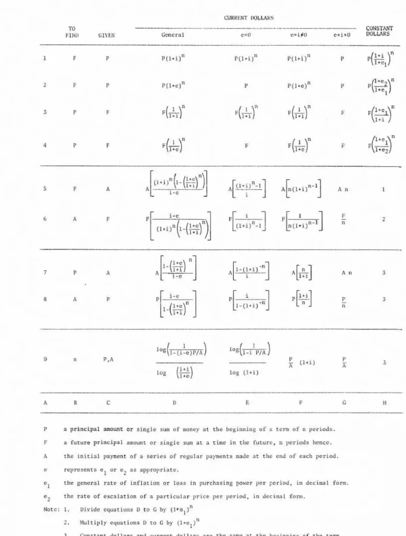
The most common equations used i n life-cycle c o s t i n g a r e s e t f o r t h

i n Table 1 . The equations have been grouped in combinations of F , P, A, and

n; i f any two of these are knorm, t h e o t h e r s can be calculated.

In t h e subsequent discussions and examples, t h e e q u a t i o n s are i d e n t i f i e d by t h e i r position in t h e Table, i.e., their line and column coordinates.

Standard interest t a b l e s , which ignore i n f l a t i o n , r e f e r t o t h a t past of t h e equation enclosed by [ ] in column E a s a p a r t i c u l a r F a c t o r . In t h e case of e q u a t i o n 7E, t h e f a c t o r i s t h e P r e s e n t Worth Factor and i s defined a s t h e present v a l u e of an annuity of u n i t value per p e r i o d f o r a t e r m of n periods at a rate of i n t e r e s t , i , p e r p e r i o d .

Columns D to G are used when t h e answer i s r e q u i r e d in current dollars and column H when r e q u i r e d i n constant d o l l a r s . Column

D

equations s h o u l d h e used i n a l l cases except when e is eqtral t o i, in which case an equation in column

F

o r G should be u s e d .

The f i r s t g r o u p o f e q u a t i o n s involving the present and f u t u r e vaIue of n s i n g l e sum has heen divided i n t o two sub-groups. Equntions 1 and 3 a r e standard e q u a t i o n s llscd t o calculnte p r e s e n t and f u t u r e values of a single

sum a t compound interest. I'quations 2 and 4 a r c used t o calculate t h e present and f u t u r e values o f an item w i t h an e s c a l a t i n g p r i c e .

The relationship between an e s c a l a t i n g series o f annual d e p o s i t s

n

A(1 + e2) . and T h e i r future sum is given i n l i n e s 5 and 6 while the

equations In Lines 7 and 8 give t h e i r relationshi? w i t h a present sum.

When t h e d e p o s i t A does not e s c a l a t e , t h e equations give the amount of

an annuity and the present value of an a n n u i t y r e s p e c t i v e l y . Figure I

is a graphical representation o f the following explanation concerning

the combination of these equations.

Suppose that some energy conservation measure saves a constant q u a n t i t y of energy Q each year f o r n years. The present u n i t p r i c e of energy is C, which is e s c a l a t i n g at a yearly r a t e e ₂

_'

and t h e current i n t e r e s t r a t e i s i. What i s t h e present value of n years of savings?

The value of the f i r s t year's saving CQ is A and is available for deposit at the end of year I . The second year's saving i s increased by (1 + e2)

I1 + c,'] L

saving i s A / ( l + i ) , , t h e second year's saving is A

2 ' and t h e n t h (1 + i )

n - 1

(1 + e * )

year's s a v i n g is A

.

The sum of t h e s e (n - 1) terms i s

(1 i- i] n

L

i - e ₂

When e2 = i t h i s expression i s indeterminate. Figure 1 shows, however, t h a t in this case the present value o f each year's saving i s o n l y

The same result can be obtained by summing t h e f u t u r e values of t h e s a v i n g s at t h e end of year n and t h e n d i v i d i n g by (1

+

i)" to o b t a i n t h e p r e s e n t v a l u e

.

If t h e r a t e of escalation e of the p r i c e of energy is t h e same as

2

t h e g e n e r a l r a t e o f i n f l a t i o n e , then el can be substituted f o r e

2.. - I n

this case, t h e r a t i o o f c o n s e c d i v e terms becomes (1 + e ) / ( 1 + i) r h l c i l

i s equal to (1 + y) the e f f e c t i v e i n t e r e s t r a t e . The value of the first t e r n , however, i s s t i l l A / ( 1 + i) and not A / ( 1 + y ) , that is t o s a y (1 + e l )

is missing from t h e first term sf the series. Consequently, t h e r e is no advantage in e s t i m a t i n g y t o avoid e s t i m a t i n g e and i separately because

1

i must b e estimated in o r d e r to calculate thc correct present v a l u e .

The equations given i n l i n e 9 for calculating the payback p e r i o d can

only be used i n simple cases t h a t involve oniy one investment and an

annual saving. If a f a c t o r such as annual maintenance is a l s o considered,

line 9 equations can s t i l l be used p r o v i d i n g t h e escalation sates f o r t h e energy savings and t h e maintenance c o s t s are the same, When they are different, a high estimate can b e o b t a i n e d by u s i n g t h e l a r g e r of t h e i n f l a t i o n and e s c a l a t i o n values for e

i n

equation 9D. In this and more complicated cases, a net cash flow analysis s h o u l d be c a r r i e d out.

L i n c 9 cquarions show thaz n i s dependent on t h e ratio P/A, Equations 9 D and 9 E become indeterminate when [i - e ) P / A i s g r e a t e r than 1 because one c a n n o t o b t a i n the log of a negative number. Tn this case, and a l s o when

( i - e ) P / A i s equal t o 1, the payback period n is infinite. It is interesting

to note that for r e a s o n a b l e values o f P, A , i and e , equations 9D, 9F and 9G will givc reasonably similar payback p e r i o d s , b u t i f t h e i n f l a t i o n or

cscalation r a t e is ignorcd, i.e., e = 0, equation 9E may be i n d e t e m i n a t e and

Thc i n t e r n a l rrtte of r e t u r n method is an n l t c r n n t i v e to thc u s e of t h e payback p e r i o d as a means o f comparing different i n v c s t r n c n t s

or o f determining if a particular investment is economically d e s i r a b l e . It i s d e f i n e d as t h a t rate o f return, i.c., interest r a t e that, when

applied to both t h e c a p i t a l investment and the periodic s a v i n g s , will produce t h e same future w o r t h at t h e end of n p e r i o d s of time. The

difference between t h i s and the p r e v i o u s method is t h a t in the former t h e

interest rate is assumed and t h e payback period n calculated, w h i l e i n t h i s second method the p e r i o d n i s assumed and t h e interest r a t e

is

calculated. T h i s is a h y p o t h e t i c a l s a t e o f r e t u r n t h a t g i v e s a c l e a r

indication o f the relative v a l u e o f a l t e r n a t i v e investments and a v o i d s t h e more difficult task o f e s t i m a t i n g t h e future value of money.

The use of the internal rate o f r e t u r n mctllod i s limited to simple cases;

thc p r o c c d u r c i s o s follows.

1 . Calculate t l ~ c prcscnt worth f a c t o r , W x , by thc cqkrntion

2. Read o f f t h e i n t e r e s t rate x, expressed a s a decimal, corresponding to Wx

and n from Figure 2 or determine x by t r i a l and error by means of

equation T E as follows:

TABLE 1. LIFE-CYCLE COST EQllATTONS CURRENT IbVLLAR5

5 F A

i-c A n 1

P a principal mount or s i n g l e sum o f moncy at t h e beginning of a t e n of n p e r i o d s . F a f u t u r e principaI amount or s i n g l e sum at a timc i n rlrc f u t u r e , n ~ l e r i o d s hencc.

A t h c r n i t i a l payment of a series of regular payments made a t t h e end nf e a c h pcriod.

e represents c O T e Z a s approllriatc.

the gencral r a t e o f i n f l a s i o n or loss i n purchasing power per period, in decimal form.

e2 t h e r a t e a f escalation o f a past~cular price per period, in decimal form.

Notc: 1. D i v i d e equations D ta G hy [ I + @ )"

1

1. Multiply equations O t o G by [l+cl)"

Yc;l r No.

Year End

A

1 A (1

_I

+

5 1

I

A { i +

_I

e,)n-l -

I

₁

I

Present Value o f Savi-ngs

I

I

I

I

-

- = P, the p r e s e n t v a l u e o f an escalating s e r i e s

i - e of payments or s a v i n g s

Note: Because t h e series of values i s a geometric s e r i e s , t h e sum of the

present values P can be calculated by the equation

P = a (1

-

rn)

l - r

where a = t h e v a l u e o f t h e f i r s t term = A / ( 1 + i] and

x = t h e r a t i o between any two terms = (I + e ₂ ) / ( I + i)

FIGURE

1

P R E S E N T W O R T H F A C T O R . W x

FIGURE 2a

INTERNAL

RATE OF RETURN, PRESENT IVORTH

PRESENT W O R T H F A C T O R , W x

FIGURE 2b

Thc following examples a r c given to illustrate the usc o f t h e v a r i o u s

equations.

Example 1

A device that will reduce water consumption in a house hy 4 . 5 L pcr person per day is available at a cost of $ 5 . It has a l i f e expectancy of at least 20 years. Hater currently c o s t s 20$Jm3 and its price is expected

to escalate at an annual rate ( e ) of 5%. Bank i n t e r e s t (i) is 7% on savings. There are 4 persons in the family and t h e householder will install the

device at no extra cost. IVhat is [a) the f i r s t yeas's savings, [b) t h e present value of such an investment, (c) t h e future value of t h e return on the investment, [d) the payback p e r i o d and ( e ) the internal r a t e of r e t u r n on

t h e investment?

(a) t h e f i r s t year saving i s

(b) The present value i s (equation 7D)

( c ) The f u t u r e value of the return on the investment F is equal to (I) the f u t u r e value of t h e annual savings (equation SD) l e s s

the future value o f the i n i t i a l investment (equation 2D)

( 2 ) the future value o f the difference between the p r e s e n t valuc

of the savings and the initial capital investment (equation I n )

[dl The payback period i s (equation 9n)

(e) The i n t e r n a l rate o f return [r] is:

y = 0.25 from Figure 2

r = 1.05 x 0.25 + 0 - 0 5 = 0 - 3 1 (31%)

A new bungalow i s being b u i l t in the Ottawa area a n d is t o b e h e a t e d by

means of an oil-fired warm air furnace. The owner would like to know

(a) Haw much insulation should be put i n ~ t h e c e i l i n g ? (b) How much will it c o s t ?

( c ) How much will h i s annual f u e l b i l l be reduced?

(d) How long will it take him to recover h i s investment in insulation?

(e) What will be the internal rate o f r e t u r n an h i s investment?

The bungalow h a s an area (a) of 110 m2 and the ceiling construction has a thermal r e s i s t a n c e ( R l ] of 0.50 r n 2 ° ~ / ~ . Insulation i s t o be blown

cellulose w i t h a thermal resistance of 19.75 rnZ0c/h' p e r metre o f thickness.

It will c o s t (bz] $ ~ . 7 6 5 / m 2 p e r u n i t of r e s i s t a n c e plus a set-up cost o f

[ b l ) $1.08/m2. Fuel c o s t s [z) are $0.137JL with

a

heat content (F) of

1 0 . 8 3 3 kW.h/L (39 M J j L ) . The furnace has a seasonal efficiency of

utilization

[El

of 0.70. O t t a w a h a s a h e a t i n g season (D) of 4853 degree d a y s and experience h a s shown that a correction f a c t o r

(C)

o f 0.75 i s

required to compensate f o r extraneous h e a t gains. The bungalow has a life expectancy (n) of 50 years. During t h i s time it is expected t h a t t h e c o s t o f f u e l o i l will escalate at an average rate (el of 0.08 and that t h e

[a) The optimum amount of insulation (R2] to be added may be

calculated by means of t h e equation:

where the present worth factor CW) is taken from equation 7D as

W =

i - e

W = = 30.02, and

[b) Cast of insulating the c e i l i n g may be calculated by the equatian

C.

= (bl + b2R2)a

1

( c ) The reduction in f u e l c o s t (A) for t h e f i r s t year may be calculated by the equation

I _{A - 4}

[d) The payback period (11) is calculated using equation 9D

1 log ( 0 . 1 0 - 0 . 0 8 ) 7 4 1 . 5 1 I

-

n = 325.13 = 2.5 years 1-10 l o g

-

1.08

( e ) The internal rate of r e t u r n (r] is calculated by the proccdurc

g i v e n previously.

{ i i ) Since Wx i s small, the t r i a l and error method is used and

gives

(iii) r = (1 + el x + e

r = 1.08 x 0 . 4 1 + 0.08 = 0 . 5 2

Readers should note t h a t t h e saving is t a x free. To rake a d i r e c t

comparison w i t h t a x a b l e investment income, the t a x Frce savings s I ~ o u l d be increased by d i v i d i n g by 1 minus the applicable Tax r a t e

in

decimal

form.

As t h i s example shows, t h e i n t e r n a l r a t e of r e t u r n i s very large and t h e payback period corrcspondingly s h o r t when a building i s i n s u l a t e d t o its optimum l e v e l of thermal resistance. The reason is t h a t evcry

added unit o f resistance, except. t h e last u n i t , more t h a n pays f o r

i t s e l f because, by the definition of optimum l e v e l of r e s i s t a n c e , t h e l a s t u n i t of r e s i s t a n c e added j u s t saves enough t o pay f o r i t s e l f .

In many cases, the theoretically optimum thermal resistance cannot

b e added and the owner i s faced with a choice o f w h e t h e r t o u n d e r - i n s u l a t e

or over-insulate. In both of t h e s c cases, the i n t e r n a l rate of r e t u r n

will be l e s s t h a n t h a t corresponding to t h e optimum. The owner can c a l c u l a t e b o t h cases and choose t h e most economical. It i s recommended

that t h e higher level of insulation be chosen, as this will save more

e n e r g y and will b e more economical i f t h e f u t u r e energy c o s t s turn out t o be underestimated.

Example 3

The owner of a 10-year o l d bungalow in Ottawa wants to upgrade the insulation in the attic which i s t h e o l d RLO b a t t s with a r e s i s t a n c e of I . 76

m2"c

J W . The house i s similar to t h e house in t h e previous cxample

and t h e same details and c o s t f a c t o r s apply except t h a t t h e thermal

r e s i s t a n c e of t h e ceiling is 2.25

rn2"c/IV.

'lke owner i s i n t e r e s t e d in answers t o t h e same q u e s t i o n s as i n t h e previous example.

(a) Because the d e t a i l s and c o s t f a c t o r s a r e t h e same as in tllc pr~vious cxample, t h e optimum thermal r e s i s t a n c e of t h e c e i l i n g (KO) i s t h e

same. The amount t o be added (R2) i s much smaller because some

i n s u l a t i o n i s already i n place. The amount t o be added is

(b) Cost o f installing the i n s u l a t i o n

( d ) Thc payback period (n) i s [ c q u n t i o n CJD]

1

log

(0.10

-

0.08) 594.25

1 -

n = 55.16 = 1 3 . 2 years

(e) The internal r a t e of return i s

5 9 4 m 2 5 = 1 1 . 6 3

(i)

W = 1.08 x 5 5 b 1 6

X

(ii] From Figure 1 , x is 0.085

(iii) r = 1.08 x 0.085 + 0.08 = 0.172

o r a 17.2% annual r a t e of return

A house i s being designed f o r an owner who i s wondering about t h e

economics o f i n s t a l l i n g a h e a t pump as an a l r e r n a t i v c t o an electric forced-

air furnace. While the h e a t pump will provide a i r c o n d i t i o n i n g in t h e swmner, all t h e c a p i t a l and maintenance c o s t s are to be charged a s h e a t i n g

c o s t s . The h e a t pump system will c o s t $2000 more to install t h a n t h e electric furnace system and will have a seasonal performance factor of 1.5. Annual

maintenance c o s t s w i l l be increased by $30 with t h e heat pump. The compressor in the heat pump has a l i f e expectancy o f 10 years and it currently costs $400

to replace one. The house and a l l other components have a 50-year life

expectancy. The current cost of electricity is 2.5#/klV-h and it is estimated t h a t 22.4 M!V-'h sf electricity will b e r e q u i r e d by t h e electric furnace d u r i n g t h e heating season.

Because one must allow f o r replacing t h e compressor every 10 y e a r s , it i s

convenient t o forecast changes in t h e i n t e r e s t and i n f l a t i o n r a t e s an a s h o r t

term b a s i s f o r the f i r s t 10 years and on a long term b a s i s covering t h e l a s t

40 years. The various rates are tabulated as follows:

Rate Symbol 0-10 yrs 11-50 y r s I n t e r e s t an money

i

0 . I 0 0 - 0 7

General

inflation 0.07 0.04 E s c a l a t i o n of electricity e 2 0.09 0.06

This problem can be solved by calculating thc n e t p r e s e n t worth of t h e heat pump relative to t h e e l e c t r i c furnace. If t h e answer is positive then t h e h e a t pump is more economical. Of c o u r s e , t h e heat pump will always use

Savings :

( a ) F i r s t yearfs saving in electrical c o s t

(b] P r e s e n t worth o f s a v i n g s during t h e first term (equation 7D)

(c) Present w o r t h of savings during t h e secorld term (equ~tions 2D, 713 and 311)

(d) Total present worth o f e n e r g y savings = $6964.08

C o s t s :

(a) Increased capital cost of heat pump P = S2000

H -

(b) (i) Present worth o f r e p l a c i n g t h e compressor a t end o f first

term (equations 2D and 3 D )

1 07 1 0

PCl = 400 x (-) = $303.37

1.10

(it) Present w o r t h o f r e p l a c i n g the compressor t h e second time

( i v ) P r e s e n t worth of replacing t h e compressor t h e f o u r t h time

(v) Because the life of the house is estimated at 50 years, t h e r e

is no need to replace the compressor 8 f i f t h time and no

c o s t i s incurred.

[vi) T o t a l present w o r t h of replacing compressors = $S32.69 [ c ) (i) Present worth of i n c r e n s e d maintenance c o s t s f o r t h e f i r s t

term (equation 7D)

(ii) Present worth of t h e increased maintenance c o s t s f o r the

second term (equations 2 D , 7D, and 3D)

(iii) Total present worth o f increased maintenance c o s t s = $756.83

Total p r e s e n t worth of a l l c o s t s = $3589.52

The n e t present worth of the heat pump relative t o an electric forced-air

furnace f s $6964.08 - $3589.52 = $3374.56.

The h e a t pump is t h e r e f o r e more economical than t h e electric furnace

and will reduce the consumption of electrical energy by one t h i r d . The r e s u l t s o f the economic comparison arc dependent on t h e assumed interest,

i n f l a t i o n and energy escalation r a t e s m d t h e period o f time chosen.

If the period chosen had been only 10 years, then t h e present w o r t h

o f the savings

would

be $1629.14 and t h e present worth of the c o s t s $2000.00 + $ 2 4 1 - 5 7

f o r

a total of $2241.57. This gives a net value o f $ 6 1 2 . 4 3 in favour of t h e electric furnace.

'[here i s no simple way to calculate the payback period o r thc intcrnal rate o f return f o r this examplc. A cash flow a n a l y s i s shows, however, t h a t t h e minimum investment required i s $2000 f o r t h e heat pump p l u s a fund o f $144.64 to cever e a r l y d e f i c i t s in t h e savings. Savings in electric energy c o s t s a r e used to cover t h e increased main~enancc c o s t s and any s u r p l u s c r e d i t e d t o the investment fund. The i n i t i a l deposit in the investment fund will g e n e r a t e svfffcient money to cover t h e initial d e f i c i t s in t h e yearly savings and t h e t o t a l c o s t of t h e first compressor replacement a t t h e end of

1 0 years. By the end of 16 years, it will have accumulated enough money to

pay o f f the $2000 heat pump investment with interest and have $168.55 l e f t

over. T h i s amount plus subsequent surplus savings will cever f u t u r e

compressor replacements and produce a surplus o f $136,685 at the end of t h e

50-year p e r i o d . The present w o r t h of this amount is $3519.20 and i s made up nf thr prcscnt w o r t h of t h c heat pump system o f $3374.56 p l r ~ s t h e initi:rT