HAL Id: hal-00919142
https://hal.inria.fr/hal-00919142
Submitted on 16 Dec 2013
HAL is a multi-disciplinary open access
archive for the deposit and dissemination of
sci-entific research documents, whether they are
pub-lished or not. The documents may come from
teaching and research institutions in France or
abroad, or from public or private research centers.
L’archive ouverte pluridisciplinaire HAL, est
destinée au dépôt et à la diffusion de documents
scientifiques de niveau recherche, publiés ou non,
émanant des établissements d’enseignement et de
recherche français ou étrangers, des laboratoires
publics ou privés.
Spatio-temporal registration of embryo images
Léo Guignard, Christophe Godin, Ulla-Maj Fiuza, Lars Hufnagel, Patrick
Lemaire, Grégoire Malandain
To cite this version:
Léo Guignard, Christophe Godin, Ulla-Maj Fiuza, Lars Hufnagel, Patrick Lemaire, et al..
Spatio-temporal registration of embryo images. ISBI - International Symposium on Biomedical Imaging, Apr
2014, Pekin, China. �hal-00919142�
SPATIO-TEMPORAL REGISTRATION OF EMBRYO IMAGES
L. Guignard
⋆†C. Godin
†U.-M. Fiuza
⋆L. Hufnagel
‡P. Lemaire
⋆G. Malandain
§⋆
CRBM, UMR 5237, CNRS, Univ. Montpellier 1 & 2, 34293 Cedex 5 Montpellier, France
†Inria, Virtual Plants team, UMR AGAP, 34095 Montpellier, France
§
Inria, Morpheme team, 06900 Sophia Antipolis, France
‡EMBL, Cell Biology and Biophysics Unit, Heidelberg, Germany.
ABSTRACT
Current imaging techniques can capture temporal sequences of 3D images with very high time resolution over several hours. Com-paring sequences covering the same time period opens the way to the study of developmental variability. Stitching together sequences captured from different embryos may help producing a sequence covering the whole development of the animal of interest. For this, it is necessary to align two sequences in both time and space.
We present here a method to align two 3D+t time series, based on the detection and pairing of 3D+t landmarks. These landmarks, which correspond to periods of fast morphogenetic change, are de-duced from the analysis of the non-linear transformations that allow to co-register pairs of consecutive 3D images in each sequence.
Index Terms— Image registration, Image sequence processing, Fluorescence microscopy, Light sheet microscopy, Embryogenesis, Morphogenesis
1. INTRODUCTION
Animal and plant morphogenesis is a highly dynamic process span-ning several temporal and spatial scales. One challenge is to describe cell and/or embryo shapes through development, to analyze their dy-namics and variability within and between species and to correlate this information with gene activity [1, 2]. For this, it is necessary to compare the development of several embryos in order to identify similarities and variations in morphogenetic events.
Recent progress in light microscopy allows the capture of 3D images of entire live embryos at a sub-cellular level of resolution with a high rate of acquisition and without interfering with devel-opment [3]. These protocols produce 3D+t images depicting the development. Comparing or fusing such sequences captured from different embryos is a challenging task, but of crucial importance. While it is generally not possible to image an embryo throughout its whole development, one can generate developmental sequences from different individuals, with partial temporal overlap. Stitching together such time series can be used to produce a consensual repre-sentation of the whole development, and would also allow to identify variations in these programs.
There are however two main challenges. Firstly, it is experimen-tally difficult or impossible to orient the embryos in a standardized manner during imaging. Moreover embryos often progressively drift in the field of view during long time-lapse sessions. It is thus nec-essary to realign spatially each sequence so that the embryos are in the same orientation, and thus can be easily compared. Secondly, one needs to temporally align these time series over their periods of overlap. Because of the very large size of such datasets (up to several
hundred 3D images per sequence), alignment methods have to be as automated as possible.
We propose here a landmark-based registration method for two 3D+t time series. These landmarks are extracted from the analysis of the sequences. More precisely, in a given time series, every pair of consecutive 3D images are co-registered with a non-linear transfor-mation, and the largest regional deformations are extracted from the whole sequences, yielding 3D+t landmarks. Alignment of two inde-pendent sequences is then achieved by finding the optimal pairings between two sets of 3D+t landmarks.
2. DATA DESCRIPTION
We used the simple marine invertebrate chordate Phallusia mammil-lata (P.m.) to test and develop our algorithms. Embryonic develop-ment of this species is highly similar across individuals, because the timing and orientation of cell divisions are highly stereotyped. As a consequence all cells can be unambiguously named and recognized up to the 112-cell stage, when the first major morphogenetic process, gastrulation is initiated.
We imaged live embryos using a lightsheet microscope (Mu-ViSPIM, EMBL, Heidelberg [4]). To image membranes, embryos were soaked in a lipophilic dye (FM4-64). The dye was excited with a 594nm laser (Cobolt AB) and the emitted light was collected by two opposing 25x Nikon water dipping objective lens (NA 1.1) and after passing thought a long-pass filter (BLP01-594R-25, Sem-rock), was collected with a Hamamatsu Flash 4 SCMOS camera. At each time point, two perpendicular 3D image stacks, each with 1200 × 1200 pixels per plane and a total of 200 planes were ac-quired by both cameras. This resulted in a total of four views (0, 90, 180, 270 degrees) of the specimen each with a lateral resolution of0.26µm × 0.26µm and 1µm plane spacing. This procedure was repeated every two minutes. To obtain an 3D image with isotropic resolution, the 4 image stacks were fused into a single 3D dataset as described in [5].
For the purpose of this paper we will use time-series from two different embryos, each counting 50 time points (1h40 min). Both time series start at the 32-cell stage and end after the 112-cell stage. The imaging temperatures were different (20◦C and18◦C) so
that both embryos exhibit slightly different developmental kinetics. Fig. 1 depicts 2D sections of some 3D images at different time-points extracted from one sequence as well as the corresponding 3D renderings.
Fig. 1. Phallusia mammillata embryo from32 cells stage to 112 cells stage, 100 minutes later. The first row shows the 3D renderings of the voxel images (Amira) every 4 minutes, while the other rows display respectively some magnified views and corresponding cross-sections.
3. INTRA-SEQUENCE REGISTRATION 3.1. Registration method
Registration is a frequently addressed issue in the literature [6, 7]. Although the choice of a particular registration method may not be critical, it is important that the chosen method would be robust with respect to topological changes. For that reason, we chose to use a block matching scheme [8] to compute either linear or non-linear transformations. Such a scheme is comparable to the ICP method [9] except that iconic primitives are matched instead of points.
Registration aims at the computation of the transformation TF←R that will allow to resample a floating image IF onto a
reference image IR. The transformation TF←Ris iteratively
com-puted by integrating incremental transformations δTi, ie TF←Ri+1 = δTi◦ Ti
F←R.
At iteration i, blocks bRof the reference image IRare compared
to blocks bFof the floating image IF, the best block pairing (the one
that yields the best iconic measure, here the normalized correlation) yield a point pairing,(cR, cF), by associating the block centers. The
incremental transformation is then estimated by
δTi= arg min δT X cF − δT ◦ T i F←RcR 2 (1)
Linear transformations are computed with a Least Trimmed Squares [10] method that allows to discard outlier pairings.
The non-linear transformation is represented by a dense vector field. The transformation update follows then the following steps: 1. the sparse pairing field(cR, cF) is transformed into a dense field
by Gaussian interpolation (this Gaussian interpolation also acts as a fluid regularization); 2. outlier pairings are discarded; 3. the remain-ing pairremain-ings are transformed into a dense field by Gaussian interpo-lation; 4. this dense field is composed with the transformation found at the previous iteration; 5. the resulting transformation is smoothed by a second Gaussian filter that acts as an elastic regularization.
3.2. Pairwise registration
Consider a temporal sequence of 3D images,{It} for t = 1 . . . N .
We aim at co-registering a pair of images captured at two differ-ent time points (i.e. It and It+δt). Since a δt of 2 minutes does
not capture deformation of sufficient magnitudes we choose δt= 4 minutes. We want to be sure to capture sufficient deformations to identify cell division events.
We first co-register every pair of successive images of the time series with a rigid transformation : 3D translation + rotation repre-senting (and then allowing to compensate for) the small
displace-ments of the embryo that may occur during the acquisition. Hence, we get a series of rigid transformations Rt←t+δtallowing to
resam-ple Itonto It+δt.
To compensate for the displacements along the whole sequence, a reference image is chosen (here IN), and all the transformations
Rt←Nare calculated by transformation composition, which allows
to resample all Itimages into INframe
IN←t= It◦ Rt←N= It◦ Rt←t+δt◦ . . . ◦ RN−δt←N (2)
From now on, it is assumed that the sequence is compensated for the small rigid displacements (ie IN←tis now denoted It).
The remaining deformations that exist between two successive images can be captured thanks to a non-linear registration step. We then compute the non-linear transformations Tt+δt←t thereby
re-sampling It+δtin the same frame as It.
The non-linear transformation T is encoded by a vector field v such that T(m) = m + v(m), the modulus of the vector v(m) indicating the local amount of variation at point m. Fig. 2 depicts such a vector field calculated from the registration of 3D images at two successive time-points: it demonstrates that the deformations are regionally localized, suggesting that these areas are of interest from a morphogenesis point of view.
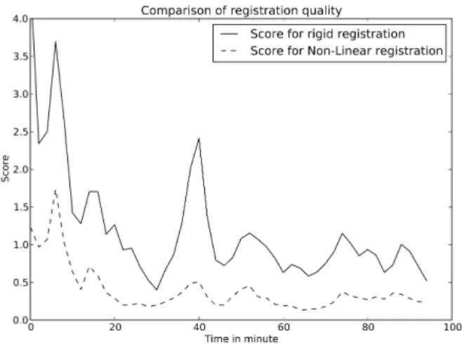
3.3. Registration assessment
To assess the registration quality, we used a distance between the two images based on a comparison of membranes location. The distance is small when the membranes are mainly overlaping. For this, we take advantage of the dye that makes the membranes hyper-intense and extract them by thresholding. More precisely, 10% on average of the image represents membranes, so the membrane setM(I) of image I is defined by the binary image resulting of the thresholding of I by the intensity representing the90thpercentile of the cumula-tive histogram. Although not perfect, such a membrane definition is sufficient for a rough registration assessment.
Let IF and IRbe respectively a floating and a reference image,
TF←Rthe non-linear transformation from IRto IF, IF→Rthe
float-ing image resampled onto the reference one (IF→R= IF◦ TF←R),
and MR and MF→R the membrane sets of respectively IR and
IF→R. We define a registration score S by measuring the average
distance from one membrane set to the other thanks to S(IF→R, IR) = 1 |MR| X m∈MR min m′∈M F →R kmm′k (3)
Fig. 3 shows the evolution of this score from rigid registration, ie S(It+δt, It), where the small rigid displacements have already been
Fig. 2. A cellular division occurs between 16 minutes (rendering at left) and 20 minutes (rendering at right (Amira)) for the embryo of Fig. 1. The non-linear registration that co-registers both images exhibits some high deformations, represented by large vectors (at the middle; only vector with a norm greater than7.5µm are displayed).
Fig. 3. Registration score over time for both rigid and non-linear registration.
4. ALIGNEMENT OF INDEPENDENT 3D+T TIME SERIES 4.1. Definition of 3D+t landmarks
The development of the embryo is punctuated by regional deforma-tions at precise steps. For example, during the cell division process the dividing cells round up, which causes local deformation. Also, during gastrulation part of the embryo invaginates, a process that creates regional deformations. We use these spatially and tempo-rally localized events as 3D+t landmarks to guide the co-registration of two morphogenesis sequences.
We then propose to use the deformations extrema as 3D+t land-marks. Let us denote the set of landmarks to be built byL = {Li}.
A 3D+t landmark Liis defined by a time tiand a spatial position xi.
Let us consider a temporal sequence of 3D images,{It} where the
small rigid displacements have been compensated for, together with the non-linear transformations Tt+δt←t.
We start by detecting the temporal extrema of the deforma-tions. We compute the cumulative histogram of the vector modulus kv(m)k (recall that the non-linear transformation is encoded by a vector field) for the membrane points m ∈ M(It), calculate its
90th percentile, and propose as deformation score (D(T t+δt←t))
the ratio between the mean value of the vector modulus computed on the 10% membrane points having the largest vector modulus (set denoted byM10↑), and the mean value of the vector modulus
computed on the 90% membrane points having the smallest vector
Fig. 4. Score of local deformation over time for the two embryos to be co-registered.
modulus (set denoted byM90↓) :
D(Tt+δt←t) = X m∈M10↑(It) kv(m)k |M10↑(It)| X m∈M90↓(It) kv(m)k |M90↓(It)| −1 (4)
This deformation score exhibits some extrema with respect to time (Fig. 4), which correspond to the time positions of our 3D+t land-marks, denoted by ti = t(Li). From now on, we assume that the
landmarks are temporally ordered, ie i < i′⇔ ti< ti′.
For each of these particular time points, we now compute the connected components of M10↑, retain the largest of them (this
somehow corresponds at extracting the largest, or extremal, defor-mation), and compute the center of mass of this largest connected component: this yields the spatial positions of our 3D+t landmarks, denoted by xi= x(Li).
4.2. Sequences co-registration
Let us consider two morphogenesis time series{It} and {It′′} and
their associated landmarksL = {Li} and L′ = {L′j}. To
reg-ister the two time series, we build and test pairing hypothesis be-tweenL and L′, this pairing hypothesis is included in the powerset
P(L × L′).
A pairing hypothesis H = {(iH, jH)} consists of a set of
cou-ples representing the landmark pairing{(LiH, LjH)}. Pairing
hy-pothesis are not all tested, and we retain only those obeying: 1) at least 5 landmarks have to be effectively paired; 2) pairings are temporally consistent, ie for two pairings(iH, jH) and (i′H, jH′ ), if
iH< i′Hthen jH< j′H(recall that the landmark indexes are
tempo-rally ordered). Given a pairing hypothesis, the rigid transformation registering the paired landmarks can be easily estimated in the least squares sense : TH= arg min T X {(iH,jH)} T(xiH) − x′jH 2 (5)
The mean of the residuals measures the hypothesis registration qual-ity, allowing to define the best pairing hypothesis, ˆH, by
ˆ H= arg min H 1 |H| X {(iH,jH)} TH(xiH) − x ′ jH 2 (6)
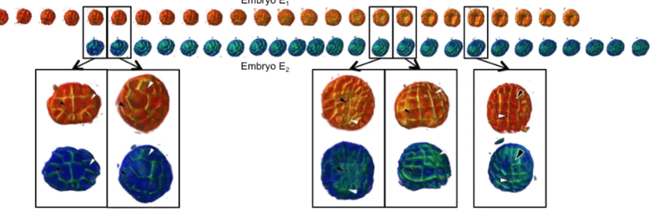
Fig. 5. Spatio-temporal registration of two time-series of embryo. Enlarged renderings indicate the registered times{(tiHˆ, t
′
jHˆ)}. Notice that
the temporal registration is not linear since the interval length between two registered time is different from one embryo to the next.
yielding not only a spatial co-registration of both sequences thanks to THˆ but also a temporal co-registration thanks to the couples
{(tiHˆ, t
′
jHˆ)}. This temporal co-registration is sparse, since only a
few time-points are co-registered. A dense temporal co-registration (where all time-points are co-registered) can easily be induced by simple means (e.g. linear interpolation) although more sophisticated schemes are under investigation.
Last, the spatial transformation between the two sequences is re-fined twice. First, we re-estimate THˆ with a Least Trimmed Squares
optimization (which discards the worse pairings out of{(iHˆ, jHˆ)}).
Second, we resample the images Ij′Hˆ using THˆ and co-register the
resulting images Ij′Hˆ ◦ THˆ with the images IiHˆ. It yields a
num-ber of transformations T(I′
j ˆH◦THˆ)←Ii ˆH. Averaging them allows to
get the spatial transformation T{I′
t′}←{It}that aligns the sequence
{I′
t′} onto {It} (see Fig. 5).
T{I′ t′}←{It}= THˆ◦ 1 | ˆH| X {(iHˆ,jHˆ)} T(I′ j ˆH◦THˆ)←Ii ˆH (7)
A visual inspection of the registered sequences demonstrates both the temporal re-synchronization of both embryos as well as the superimposition of the corresponding cells (that can be named in the first embryogenesis stages).
5. DISCUSSION
We proposed a method to spatially and temporally align two time series of embryos of P.m., with a linear spatial transformation and a non-linear temporal one. It relies on the fact that morphogenesis events, as cellular divisions, induce temporally and spatially local-ized deformations. The detection of the extremal deformations is used to build sets of 4D landmarks. Assuming that the develop-ment of different embryos of the same species is similar, landmarks identified in different embryos can be paired to eventually find the 4 dimension transformation. Our work validates this assumption in the case of the stereotyped embryos of the ascidian P.m..
By providing a spatio-temporal registration of 3D+t time series of images based on membrane deformation, our method opens the way to the geometrical quantification of morphogenesis at a cellular resolution. Finally, from this method we will be able to build longer
time series based on fusion of several overlapping smaller time se-ries.
Acknowledgment : We want to thank the Computational Biology Institute and the Fondation pour la Recherche M´edicale for partially founding this research
6. REFERENCES
[1] E Munro, F Robin, and P Lemaire, “Cellular morphogenesis in ascidians: how to shape a simple tadpole,” Curr Opin Genet Dev, vol. 16, no. 4, pp. 399–405, 2006.
[2] J Traas and O Hamant, “From genes to shape: understanding the control of morphogenesis at the shoot meristem in higher plants using systems biology,” C R Biol, vol. 332, no. 11, pp. 974–85, 2009.
[3] PJ Keller, “Imaging morphogenesis: technological advances and biological insights,” Science, vol. 340, no. 6137, pp. 1234168, 2013.
[4] U Krzic, S Gunther, TE Saunders, SJ Streichan, and L Huf-nagel, “Multiview light-sheet microscope for rapid in toto imaging,” Nat Methods, vol. 9, no. 7, pp. 730–3, 2012. [5] R Fernandez, P Das, V Mirabet, E Moscardi, J Traas,
JL Verdeil, G Malandain, and C Godin, “Imaging plant growth in 4-d: robust tissue reconstruction and lineaging at cell reso-lution,” Nat Methods, vol. 7, pp. 547–553, 2010.
[6] B Zitov´a and J Flusser, “Image registration methods: a survey,” Image Vis Comput., vol. 21, no. 11, pp. 977–1000, 2003. [7] A Sotiras, C Davatzikos, and N Paragios, “Deformable medical
image registration: a survey,” IEEE Trans Med Imaging, vol. 32, no. 7, pp. 1153–90, 2013.
[8] S Ourselin, A Roche, S Prima, and N Ayache, “Block match-ing: A general framework to improve robustness of rigid regis-tration of medical images,” in MICCAI’00. 2000, vol. 1935 of LNCS, pp. 557–566, Springer.
[9] PJ Besl and ND McKay, “A method for registration of 3-D shapes,” IEEE Trans Pattern Anal Mach Intell, vol. 14, no. 2, pp. 239–256, 1992.
[10] PJ Rousseeuw and AM Leroy, Robust Regression and Outlier Detection, Wiley & Sons, New-York, 1987.