HAL Id: hal-01370975
https://hal.archives-ouvertes.fr/hal-01370975v3
Submitted on 23 Nov 2017
HAL is a multi-disciplinary open access
archive for the deposit and dissemination of sci-entific research documents, whether they are pub-lished or not. The documents may come from teaching and research institutions in France or abroad, or from public or private research centers.
L’archive ouverte pluridisciplinaire HAL, est destinée au dépôt et à la diffusion de documents scientifiques de niveau recherche, publiés ou non, émanant des établissements d’enseignement et de recherche français ou étrangers, des laboratoires publics ou privés.
summer hot temperatures since 1851
M Carmen Alvarez-Castro, Davide Faranda, Pascal Yiou
To cite this version:
M Carmen Alvarez-Castro, Davide Faranda, Pascal Yiou. Atmospheric dynamics leading to West European summer hot temperatures since 1851. Complexity, Wiley, 2018, 2018, pp.2494509. �10.1155/2018/2494509�. �hal-01370975v3�
summer hot temperatures since 1851
2
M. Carmen Alvarez-Castro, Davide Faranda, Pascal Yiou 3
Laboratoire des Sciences du Climat et de l’Environnement, UMR 8212
4
CEA-CNRS-UVSQ, IPSL, Universit´e Paris-Saclay, F-91191 Gif-sur-Yvette, France
5
E-mail: [email protected]
6
November 2017
7
Abstract. Summer hot temperatures have many impacts on health, economy
8
(agriculture, energy, transports) and ecosystems. In western Europe, the recent
9
summers of 2003 and 2015 were exceptionally warm. Many studies have shown that
10
the genesis of the major heat events of the last decades was linked to anticyclonic
11
atmospheric circulation and to spring precipitation deficit in southern Europe. Such
12
results were obtained for the second part of the 20th century and projections into
13
the 21st century. In this paper, we challenge this vision by investigating the earlier
14
part of the 20th century from an ensemble of 20CR reanalyses. We propose an
15
innovative description of Western-European heat events applying the dynamical system
16
theory. We argue that the atmospheric circulation patterns leading to the most
17
intense heat events have changed during the last century. We also show that the
18
increasing temperature trend during major heatwaves is encountered during episodes
19
of Scandinavian blocking, while other circulation patterns do not yield temperature
trends during extremes.
21
Keywords: Weather Regimes, Climate Dynamics, Heat Events 22
1. Introduction: 23
In western Europe, recent hot summers were characterized by anomalous meteorological 24
conditions. In those situations, such as 2003, the heat was prolonged and intense, and the 25
consequences were disastrous for society and ecosystems (Sch¨ar & Jendritzky 2004, Ciais
26
et al. 2005, Poumadere et al. 2005, Robine et al. 2008, Wreford & Adger 2010). 27
European surface temperature variations are influenced by processes that combine 28
radiative forcing, the large-scale atmospheric circulation and local phenomena. Over 29
the last five decades, most of the intense European heat events have been connected 30
to prolonged spells of anticyclonic circulation (Scandinavian blocking) and dry spring 31
conditions in Southern Europe (Sch¨ar et al. 1999, Fischer et al. 2007, Vautard
32
et al. 2007, Zampieri et al. 2009, Mueller & Seneviratne 2012, Quesada et al. 2012). 33
However, the Summer 2011 was cool and preceded by a dry spring; the Summer 2013 34
was warm and preceded by a wet spring; and the Summer 2015 was warm with persisting 35
southerly atmospheric flows and no lasting blocking episodes (J´ez´equel et al. 2017).
36
The goal of this paper is to assess the robustness of the link between heat events and 37
atmospheric circulation. We perform a statistical and dynamical analysis on a long 38
period that covers 1851–2014. Since anticyclones extend to a radius of few hundreds 39
kilometers, such a connection must be investigated on a regional scale (Della-Marta 40
et al. 2007, Stefanon et al. 2012). Hence, we restrict our analysis to Western Europe 41
in the region covering France and the Iberian Peninsula, whose weather conditions are 42
strongly influenced by the atmospheric circulation over the North Atlantic. This analysis 43
also puts some of the results of Horton et al. (2015) on this link into a broader time 44
perspective. 45
2. Data and Methods: 46
We base our analysis on the sea-level pressure (SLP) and the surface temperature fields 47
during summers (June-July-August: JJA) in 20th Century Reanalysis data version 2c 48
(20CRv2c: 1851–2014, (Compo et al. 2011)) with 2◦ of resolution and bias correction
49
applied in the sea ice distribution by assimilating new SST and sea-ice cover (SIC) 50
data (Hirahara et al. 2014). To ensure the robustness of the results, we used the 51
ensemble mean (EM) and the 56 members of the ensemble. The analysis is completed 52
with other reanalysis products: NCEP (1948–2016) (Kalnay et al. 1996) and ERA20C 53
reanalysis (1900–2000) (Poli et al. 2013) (see supplementary material). In order to 54
describe the variability of the atmospheric circulation, we decompose the summer SLP 55
anomalies field (obtained by removing the seasonal cycle) into four weather regimes 56
following the approach of Yiou et al. (2008) and study their connection with heat events 57
at seasonal(i) and sub-seasonal(ii) timescales in Western-Europe [10◦W – 7.5◦E; 35 –
58
50◦N]. i) Seasonal: the 24 summers with high mean temperature anomalies (with respect
59
to the climatology) of the period 1851–2014, and ii) Subseasonal: heatwaves defined as 60
periods with high temperatures anomalies for at least five consecutive days. In both 61
analyses temperatures are detrended by removing a linear trend calculated from the 62
time series of summer seasonal means. The goal of the detrending is to remove the 63
effect of the well-documented European temperature increase, which does not depend 64
on the weather pattern. 65
2.1. Weather Regimes: 66
Weather regimes are recurring states of the atmospheric circulation and provide a useful 67
description of the atmospheric variability (Michelangeli et al. 1995, Corti et al. 1999). 68
Following the methods of Michelangeli et al. (1995) and Yiou et al. (2008) we compute 69
four weather regimes (k = 4) over the North Atlantic region [80◦W – 50◦E; 20 –
70
70◦N] (Fig. 1a-d) on daily NCEP SLP anomalies (reference period: 1970–2010) over
71
the summers (June–July–August: JJA). We take the first ten Empirical Orthogonal 72
Functions (EOFs) of SLP anomalies (with weights that are proportional to the cosine 73
of latitude) and the corresponding Principal Components (PCs). Then we perform 74
a classification, with a k-means algorithm (Michelangeli et al. 1995), and a choice of 75
four weather regimes. This classification is iterated several times with random initial 76
conditions following the procedure of Yiou et al. (2008) in order to obtain weather 77
regimes that are stable. The choice of four weather regimes is to be consistent with the 78
seminal paper of (Cassou et al. 2005). For comparison, we classify different reanalysis 79
datasets with the NCEP weather regimes. All the reanalysis data are interpolated 80
onto the NCEP grid (2.5◦ × 2.5◦). The SLP data classifications of all reanalyses are 81
obtained by determining the minimum of the Euclidean distances to the four NCEP 82
summer weather regime centroids. This is achieved without further EOF truncation. 83
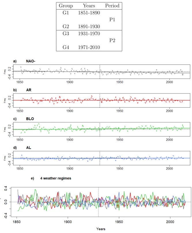
The NCEP summer weather regimes are shown in Fig. 1a-d, with the same nomenclature 84
as in Cassou et al. (2005): a) the negative phase of North Atlantic Oscillation (NAO−) 85
showing a dipole between Greenland and Northern Europe, b) the Atlantic Ridge (AR), 86
with a high pressure over the center of the North Atlantic and some common features 87
with the positive phase of NAO, c) Scandinavian Blocking (BLO), with a high pressure 88
center over Scandinavia, d) Atlantic Low (AL), with a low pressure center covering the 89
central North Atlantic. 90
91
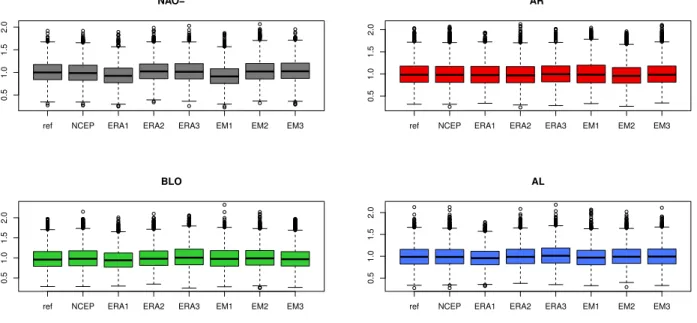
To ensure that there are no inhomogeneities in the method, we have verified 92
that the root mean square error (RMSE) between the reference period and the other 93
periods/datasets is small (Fig. S1 and Table S1). 94
2.2. Projection onto weather regimes for a dynamical representation: 95
In order to visualize the dependence between the daily SLP fields and the four weather 96
regimes, we represent the trajectory of each summer in the space of correlations (Fig. 97
3a-h) using an approach based on dynamical systems theory (Katok & Hasselblatt 1997) 98
. In this framework, the motion of a particle is represented in the space defined by its 99
position and speed (the so-called phase space). In our set-up, the particle is replaced 100
by a SLP field and the directions in phase space correspond to the projections on the 101
four weather regimes. Trajectories provide additional information with respect to the 102
monthly average statistical quantities, on the time dependence and the coherence of 103
the dynamical projection with respect to weather regime bases. If a trajectory jumps 104
every day to a different region of the phase space, then a dominant weather regime is 105
not representative of the dynamical behavior of events lasting several days. If instead 106
the trajectory occupies a restricted region of the phase space with smooth transitions of 107
the projection among weather regimes, then the dynamical representation is informative 108
and the base of weather regimes is appropriate. 109
This is equivalent to assuming the existence of a low-dimensional attractor. The 110
caveat is that the weather regime description is a first order simplification of the 111
atmospheric circulation that captures large scale features. Although this phase-space 112
method has been debated since Lorenz (1991), there is theoretical (Chekroun et al. 2011) 113
and experimental (Casdagli et al. 1991) evidence that such a procedure is effective when 114
the dynamics can be projected on a low dimensional phase space with a stochastic 115
perturbation. 116
3. Results and Discussion: 117
The link between the North Atlantic atmospheric circulation and heat events over France 118
and the Iberian Peninsula is investigated at short and long timescales. Both timescales 119
carry a physical and societal relevance. 120
3.1. Seasonal scale: weather regimes during the warmest summers 121
We carried out a statistical analysis of the hottest summers of the period 1851–2014 122
using 56 members and the Ensemble Mean (EM) of the 20CRv2c. In Western-Europe 123
[10◦W – 7.5◦E; 35 – 50◦N], the 24 warmest summers (Fig. 1e-f) are defined in each
124
dataset as the ones having the highest average temperature anomalies with respect to 125
the climatology. Figure 1e shows the probability to have a dominant weather regime, 126
which is the one with highest anomalous frequency, in each summer detected. From the 127
selection of the 24 warmest summers for each member we detect 52 different summers. 128
In order to show the agreement between the members, we calcule the probability to 129
have a summer dominated by each weather regime (Fig. 1e). We divide the number of 130
members that detects a weather regime dominating that summer by the total number 131
of members that has detected that summer as a warm summer. For instance, we find 132
that for 30 members, the summer of 1887 is one of the 24 warmest summers. For 21 133
of those 30 members NAO− is the dominant weather regime and BLO for the other 9 134
members. However, we find a total agreement within 51 members detecting 2003 as a 135
warmer summer with AL as the unique weather regime dominating the summer. Hence, 136
as figure 1e shows, there is a higher probability to find a total agreement within the 137
members after 1950, being mainly BLO the dominant regime of warmest summers during 138
the second half of the 20th century and also briefly during the end of the 19th century.
139
NAO− and AR are the most dominant regimes during the first half of the 20th century.
140
This is also evident when we study the EM (Fig. 1f-j). Figure 1f shows the dominant 141
weather regime (colors) for the warmest summers (circle size) of the EM(20CRv2c, see 142
Figure S2i of supplementary material for NCEP, ERA20C and 20CR and Figure S3 for 143
some examples of warmest summers). We have divided the warmest summers detected 144
(vertical bars and figure 1g-j) in 4 groups, in order to study the variability during short 145
periods of 30 years. Boxplots in Figures 1g-j indicate the daily frequency of weather 146
regimes by group. In groups G1 (fig. 1g), G3 (fig.1j) and G4 (fig. 1j) BLO is the most 147
frequent regime during warmest summers, while in group G2 NAO− and AR are the 148
most representatives ones. Most of the warmest summers (largest circles in Fig. 1f) 149
occur during the second part of the 20th century. As observed by Stott et al. (2004) 150
and Meehl & Tebaldi (2004), they also increase in frequency over time. 151
Figure 2a-e) (Figure S2a-d for NCEP and figure S2e-h for ERA20C) shows the 152
anomalous summer frequency of weather regimes in EM of 20CRv2c with respect to 153
the NCEP reference period. In this figure we see that NAO− is the unique regime 154
decreasing in frequency with the time, and BLO is the one increasing in frequency with 155
the time (see also Figures S4 and S5). 156
To understand such trends we decompose the average information found with the 157
statistical analysis via the dynamical representation of the warmest summers (Fig 3 and 158
Fig. S6 ), defined in section 2.2. We project the daily SLP anomaly fields (grey lines) 159
onto the 4 weather regimes (NAO− and AR regimes in Fig. 3a,c,e,g and BLO and AL 160
regimes in Fig. 3b,d,f,h). This analysis synthesizes the trajectory of the atmospheric 161
circulation during heat events (colors) in a space represented by the weather regimes. 162
Circles in the axes represents the average correlations of warmest summers. 163
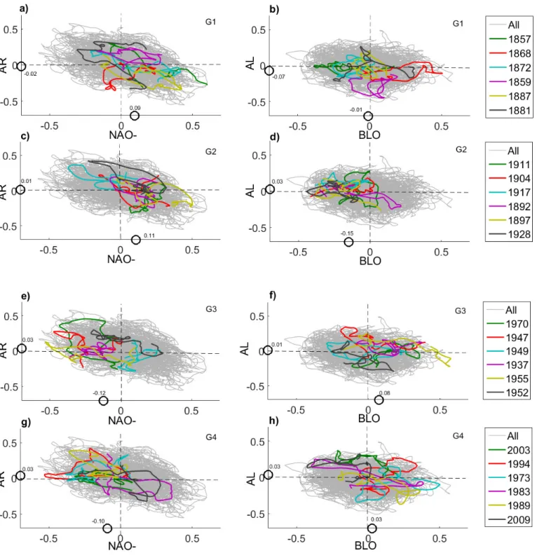
Consistently with the previous analysis, we find that the atmospheric dynamics 164
has evolved from patterns that are positively correlated with NAO− during the late 165
19th century and the beginning of the 20th century(Groups G1 and G2, Fig. 3 a,c), 166
to negative correlations during the rest of the record (Fig. 3 e,g). Similar projections 167
on BLO and AL regimes show: that BLO has the opposite change of NAO− (mainly 168
in groups G2 and G3), being negative during the early period of 20th century (Fig.
169
3d) and positive during the middle and late 20th century (Fig. 3f-h). AR and AL
170
regimes do not show significant differences between the periods. Those correlations add 171
a daily temporal information and highlight a change of atmospheric behavior. Thus 172
the dominant weather regime is a valid concept as the trajectories of heatwaves persist 173
at sub-seasonal scales around the same region of the phase space. These changes are 174
consistent within the 20CRv2c ensemble, as the analysis of the 56 members (Fig. 4a) 175
shows consistent results with the EM. In Figure 4 we represent the average correlations 176
of warmest summers as for figure 3 (circles in the axes) but for all the 56 members 177
and the EM. As for the EM, the 56 members have a positive o negative correlation 178
to NAO− and BLO depending of the period (groups in colors) being clearly separated 179
in the cloud of points the first to groups (G1 and G2, hereinafter P1) to the two last 180
groups (G3 and G4, hereinafter P2) that happens around 1930. Therefore, if we study 181
now the daily frequency of weather regimes classifying the warmest summers by only 182
two periods; before (P1) and after (P2) 1930, we find similar results as in figure 3 and 183
4a, opposite frequencies between NAO− and BLO. Higher frequencies of NAO− are 184
detected in P1 for 56 members (Fig. 4c) and the EM (Fig. 4e), and higher frequencies 185
of BLO are detected in P2 for 56 members (Fig. 4d) and the EM (Fig. 4f). 186
To complement this weather regimes analysis, we compute the difference of the 187
mean SLP for EM between these two periods during the warmest summers, ∆SLP =
188
µSLP (P 2) - µSLP (P 1). We obtain a BLO regime pattern (Fig. 4g) using the EM or 56
189
members (not shown here). This means that it is the most representative pattern for 190
the period P2, being the period P1 similar to the NAO−. 191
Therefore, our analysis shows significant changes in the dominating weather regimes 192
associated with warmest summers. If BLO is dominant from the second part of 20th 193
century, scarce occurrences of this weather regime are found before 1930, with the 194
exception of a small period at late 19th century, even within the ensemble members 195
of 20CRv2c. These results reflect a change in the regime frequencies and dominance 196
conducing to warm extremes in a multidecadal scale due to, most likely, an internal 197
variability. BLO and AL regimes are conducive to warm extremes and NAO− and AR 198
are the opposite (Cassou et al. 2005). We found that, after 1930, it is more frequent to 199
find hottest summers linked to what we know as warm regimes. BLO (the most frequent 200
one after 1930) leads to stagnant air and potential land-surface feedbacks, whereas AL 201
relies on advection from lower latitudes. In the other hand, NAO− is the dominant 202
weather regime during warmest summers up to 1930. This weather regime contributes 203
to a weakening of the westerly flow from the Atlantic into Western Europe. AR regime 204
is more stable in time. 205
3.2. Subseasonal scale: weather regimes during heatwave events 206
To understand whether those results hold also for short time events (at least 207
5 consecutive days), independently from the fact that they have been observed 208
during hot summers, we compute the average temperature during heatwaves striking 209
Western-Europe. 210
Heatwave events are defined when the summer temperature exceeds a threshold 211
based on percentiles (P90, P95) for more than 5 consecutive days. Figure 5 shows 212
heatwave events above the P95 threshold, computed on the area temperature anomalies 213
(mean of France and the Iberian Peninsula) for the 56 members (Fig 5a-d) and for the 214
EM (Fig. 5e) (See Figure S7 of supplementary material). Temperatures in figure 5 215
are average values during each heatwave event. Heatwaves events are grouped by the 216
dominating weather regime. We find that 11% of total events are dominated by NAO− 217
(Fig. 5a), 49%, by BLO (Fig. 5c). Heatwaves that are associated by AR (Fig. 5b) 218
and AL (Fig. 5d) weather regimes have a frequency of 16% and 24%, respectively. The 219
multidecadal variability in terms of frequency of weather regimes associated to warmest 220
summers is also evident in the study of summer heatwave events. The summer average 221
temperatures for Western Europe (Figure S5, supplementary material) shows higher 222
temperatures in the early and late time span. Those temperature anomalies are more 223
evident once we apply a high criteria to define heatwaves.There is a decrease in the 224
occurrence of heatwave events during the first half of the 20th century being 1930-1950 225
the only period with some heatwave events that are more frequently associated with 226
BLO regime. Although the late 19th century is dominated by BLO regime, each weather 227
regime might induce a heatwave event. However, during the late 20th century and the 228
beginning of 21st century, the NAO− regime is scarcely present during heatwave events, 229
which are dominated by AL and, mainly, BLO. We also find that the longest events are 230
associated to BLO regime (Fig. 5c,e). 231
To shed more light on the circulation changes, we compute composites of SLP and 232
surface temperature anomalies (Fig. 6) during all the days of heatwave events detected 233
in figure 5 divided by periods (table 1). Consistently with Figure 5, most of the heatwave 234
events are concentrated in periods G1 (Fig. 6a) and G4 6d) being NAO- and BLO the 235
mean pressure patterns, respectively, during those periods. There is a change also in 236
the temperature patterns mainly in Northern and Eastern Europe but also in the East 237
coast of North America and the Atlantic Ocean. Similar to G1, G2 (Fig. 6b) has 238
a NAO- as the mean pressure pattern of the period of heatwave events. Although it 239
is the period with scarce occurrence of heatwave events, G3 (Fig. 6c) is dominated 240
by a strong low pressure over the Atlantic ocean (with some influence of BLO over 241
Europe) leading to an increase in temperature anomalies in both East coast of North 242
America and West coast of Europe. Same exercise is repeated but taking into account 243
the occurrence of heatwave events pre-1930 (P1, Fig.6e) and post-1930 (P2, Fig.6f). The 244
temperature pattern changes in pre and post 1930 maps mainly in Greenland and the 245
East coast of North America and Europe (North and East). Pressure patterns for all the 246
heatwave events pre and post-1930 reproduce well NAO− and BLO-AL (respectively) 247
albeit weaker for the BLO regime which has a strong influence of AL regime (Figure S8, 248
supplementary material). So, even if there is a change for NAO−, BLO is the one with 249
a stronger change for short-term events, because it is the most representative pattern 250
in heatwave events from 1930. 251
4. Conclusions: 252
These results confirm that most heat events (either warmest summers and heatwaves in 253
Western Europe) of the second half of the 20th century occurred when the Scandinavian 254
Blocking weather regime dominated the North Atlantic region, causing increasing 255
temperatures and more frequent and longer heatwaves events (figure 5 and figure S9). 256
Our results also show that NAO− is more favorable to drive warm summers before 257
1930. This early period corresponds to the most frequent co-occurrence of this regime 258
and heatwave events. Although the increasing temperature trends observed during
259
blocking heatwave episodes could be attributed to secular climate change (Coumou 260
et al. 2014), the change in the dominating weather regimes may also be linked to the 261
decadal variability of the atmospheric dynamics. Those findings are consistent with the 262
results of Horton et al. (2015), although we consider heatwaves on a finer spatial scale 263
(Western-Europe). The analysis of Hoffmann (2017) is also complementary to ours, 264
albeit on another region (Postdam, Germany), whose temperature does not respond to 265
the same atmospheric patterns. However, he found (Figure 11) an increment of two 266
new dominant wave-like patterns with more meridional oscillation, as we have seen for 267
Western Europe at seasonal (Fig. 1, Fig. S2 and Fig. S4) and subseasonal scales (Fig. 268
5). 269
The robustness of our results is demonstrated by the use of 20CRv2c 56 ensemble 270
members and other reanalysis datasets (see supplementary material) where we have 271
found similar results. The dynamical analysis also suggests that there is an increase of 272
negative correlations between warmest summers and the NAO− regime. 273
Although the information extracted in warmest summers and heatwaves is a priori 274
different, our analysis shows similar results at different timescales. In terms of warmest 275
summers, and although there are some evidence of a multidecadal variability of the 276
atmospheric dynamic, NAO− was the most representative pattern up to 1930 and 277
from 1930 on BLO is the most representative one. For short time heat events, the 278
most representative is BLO during the whole period but, as for warmest summers, 279
NAO− events are less frequent after 1930. BLO is associated to the longest and hottest 280
heatwaves and yields an increasing trend, as outlined by Horton et al. (2015). 281
Acknowledgments: 282
M.C.A-C. was supported by the Swedish Research Council grant No. C0629701
283
(MILEX). D.F. was supported by the ERC grant No. 338965–A2C2. P.Y.
284
was supported by the European Unions Seventh Framework Programme grant No. 285
607085–EUCLEIA. The authors thank G. Compo, for the help supported with 286
data from members of 20CR reanalysis. 20CR and NCEP Reanalysis data were
287
provided by the NOAA/OAR/ESRL PSD, Boulder, Colorado, USA, and retrieved from 288
https://climatedataguide.ucar.edu/climate-data/noaa-20th-century-reanalysis-version-2-and-2c 289
and http://www.esrl.noaa.gov/psd/. ERA-20C reanalysis data provided by the
290
ECMWF (European Centre for Medium-Range Weather Forecasts), Reading, UK, 291
from their website at http://apps.ecmwf.int/datasets/data/era20c-daily/. The authors 292
declare that there is no conflict of interest regarding the publication of this paper. 293
Supplementary Material: 294
• Figure S1: Boxplots of Absolute Root Mean Square Error by period and weather 295
regime. 296
• Figure S2: Relative long-term summer weather regime frequency over the
297
North-Atlantic region and their dominance in warmest summers in Western-Europe 298
(1871-2015) using three reanalysis products (20CR, ERA20C, NCEP). 299
• Figure S3: Temperature anomalies during warmest summers in Western Europe 300
with dominance of each weather regime in three reanalysis products (20CR, 301
ERA20C, NCEP). 302
• Figure S4: 31-years running correlation of the Weather Regimes frequency and the 303
mean temperature in western Europe (20CRv2c) 304
• Figure S5: Summer average temperatures for Western Europe for three reanalysis 305
products (20CR, ERA20C, NCEP). 306
• Figure S6: Dynamical representation of the warmest summers for ERA20C during 307
1900-2010 in regimes AR-NAO- and BLO-AL. 308
• Figure S7: Dominants weather regimes during Summer Heatwave events in
309
Western-Europe for three reanalysis products (20CR, ERA20C, NCEP). 310
• Figure S8: SLP anomalies in heatwave events (20CRv2c EM) for each period, 311
• Figure S9: Temperature (y-axis) vs numbers of days (x-axis) during each heatwave 312
event for the 20CR Ensemble Mean (1871-2011) weather regimes. 313
• Table S1: Absolute root mean square error by period and weather regime. 314
Correspondence and requests for further materials should be addressed to M.C.A-C 315
(email: [email protected]). 316
References: 317
Casdagli, M., Eubank, S., Farmer, J. D. & Gibson, J. (1991). State space reconstruction in the presence
318
of noise, Physica D. 51(1): 52–98.
319
Cassou, C., Terray, L. & Phillips, A. S. (2005). Tropical atlantic influence on European heat waves, J.
320
Climate 18(15): 2805–2811.
321
Chekroun, M. D., Simonnet, E. & Ghil, M. (2011). Stochastic climate dynamics: Random attractors
322
and time-dependent invariant measures, Physica D. 240(21): 1685–1700.
323
Ciais, P. et al. (2005). Europe-wide reduction in primary productivity caused by the heat and drought
324
in 2003, Nature 437(7058): 529–533.
325
Compo, G. P. et al. (2011). The twentieth century reanalysis project, Q. J. Roy. Meteor. Soc.
326
137(654): 1–28.
Corti, S., Molteni, F. & Palmer, T. (1999). Signature of recent climate change in frequencies of natural
328
atmospheric circulation regimes, Nature 398(6730): 799–802.
329
Coumou, D., Petoukhov, V., Rahmstorf, S., Petri, S. & Schellnhuber, H. J. (2014). Quasi-resonant
330
circulation regimes and hemispheric synchronization of extreme weather in boreal summer,
331
Proceedings of the National Academy of Sciences 111(34): 12331–12336.
332
Della-Marta, P. M., Luterbacher, J., von Weissenfluh, H., Xoplaki, E., Brunet, M. & Wanner, H. (2007).
333
Summer heat waves over western Europe 1880–2003, their relationship to large-scale forcings
334
and predictability, Clim. Dynam. 29(2-3): 251–275.
335
Fischer, E., Seneviratne, S., L¨uthi, D. & Sch¨ar, C. (2007). Contribution of land-atmosphere coupling
336
to recent European summer heat waves, Geophys. Res. Lett. 34(6).
337
Hoffmann, P. (2017). Enhanced seasonal predictability of the summer mean temperature in Central
338
Europe favored by new dominant weather patterns, Climate Dynamics. .
339
URL: https://doi.org/10.1007/s00382-017-3772-0
340
Horton, D. E., Johnson, N. C., Singh, D., Swain, D. L., Rajaratnam, B. & Diffenbaugh, N. S. (2015).
341
Contribution of changes in atmospheric circulation patterns to extreme temperature trends,
342
Nature 522(7557): 465–469.
343
J´ez´equel, A., Yiou, P. & Radanovics, S. (2017). Role of circulation in european heatwaves using flow
344
analogues, Climate Dynamics .
345
URL: https://doi.org/10.1007/s00382-017-3667-0
346
Kalnay, E. et al. (1996). The NCEP/NCAR 40-year reanalysis project, B. AM. Meteorol. Soc.
347
77(3): 437–471.
348
Katok, A. & Hasselblatt, B. (1997). Introduction to the modern theory of dynamical systems, Vol. 54,
349
Cambridge University Press.
350
Lorenz, E. N. (1991). Dimension of weather and climate attractors, Nature 353(6341): 241–244.
351
Meehl, G. A. & Tebaldi, C. (2004). More intense, more frequent, and longer lasting heat waves in the
352
21st century, Science 305(5686): 994–997.
Michelangeli, P.-A., Vautard, R. & Legras, B. (1995). Weather regimes: Recurrence and quasi
354
stationarity, J. Atmos. Sci. 52(8): 1237–1256.
355
Mueller, B. & Seneviratne, S. I. (2012). Hot days induced by precipitation deficits at the global scale,
356
Proc. Natl. Acad. Sci. 109(31): 12398–12403.
357
Poli, P. et al. (2013). The data assimilation system and initial performance evaluation of the ecmwf
358
pilot reanalysis of the 20th-century assimilating surface observations only (ERA-20C), ECMWF
359
ERA Rep 14: 59.
360
Poumadere, M., Mays, C., Le Mer, S. & Blong, R. (2005). The 2003 heat wave in France: dangerous
361
climate change here and now, Risk Anal. 25(6): 1483–1494.
362
Quesada, B., Vautard, R., Yiou, P., Hirschi, M. & Seneviratne, S. I. (2012). Asymmetric European
363
summer heat predictability from wet and dry southern winters and springs, Nature Clim. Change
364
2(10): 736–741.
365
Robine, J.-M., Cheung, S. L. K., Le Roy, S., Van Oyen, H., Griffiths, C., Michel, J.-P. & Herrmann,
366
F. R. (2008). Death toll exceeded 70,000 in Europe during the summer of 2003, C. R. Biol.
367
331(2): 171–178.
368
Sch¨ar, C. & Jendritzky, G. (2004). Climate change: hot news from summer 2003, Nature
369
432(7017): 559–560.
370
Sch¨ar, C., L¨uthi, D., Beyerle, U. & Heise, E. (1999). The soil-precipitation feedback: A process study
371
with a regional climate model, J. Climate 12(3): 722–741.
372
Stefanon, M., D’Andrea, F. & Drobinski, P. (2012). Heatwave classification over Europe and the
373
Mediterranean region, Environ. Res. Lett. 7(1): 014023.
374
Stott, P. A., Stone, D. A. & Allen, M. R. (2004). Human contribution to the European heatwave of
375
2003, Nature 432(7017): 610–614.
376
Vautard, R., Yiou, P., D’andrea, F., De Noblet, N., Viovy, N., Cassou, C., Polcher, J., Ciais, P.,
377
Kageyama, M. & Fan, Y. (2007). Summertime European heat and drought waves induced by
378
wintertime Mediterranean rainfall deficit, Geophys. Res. Lett. 34(7).
Wreford, A. & Adger, W. N. (2010). Adaptation in agriculture: historic effects of heat waves and
380
droughts on UK agriculture, Int. J. Agric. Sustain. 8(4): 278–289.
381
Yiou, P. et al. (2008). Weather regime dependence of extreme value statistics for summer temperature
382
and precipitation, Nonlinear Proc. Geoph. 15(3): 365–378.
383
Zampieri, M., D’Andrea, F., Vautard, R., Ciais, P., de Noblet-Ducoudr´e, N. & Yiou, P. (2009). Hot
384
European summers and the role of soil moisture in the propagation of mediterranean drought,
385
J. Climate 22(18): 4747–4758.
in its negative phase (NAO−). b, Atlantic Ridge (AR). c, Blocking (BLO). d, Atlantic Low (AL) weather regime. e,Probability to find a dominant weather regime in all the warmest summers (EM and 56 members).f, 24 warmest summers in Western-Europe (colored region in a-d) with their dominant weather regime (20CRv2c EM). Circle size depends on temperature (anomalies), the largest the warmest. Colors represents the dominant weather regime for each summer based in the highest anomalous frequency. g-j, Boxplots of daily weather regimes during the 24 warmest summers of 20CRv2c EM (as in f ) in Western-Europe separated by groups of 6 summers per 40 years: g, shows group G1, h, group G2, i group G3, and jgroup G4 1.
Table 1. Groups and periods used during the analysis of 20CRv2c (EM and 56 members of the ensemble).
Group Years Period
G1 1851-1890 P1 G2 1891-1930 G3 1931-1970 P2 G4 1971-2010
Figure 2. Relative long-term summer weather regime frequency. Relative frequency of summer SLP (hPa) weather regimes over the North-Atlantic region (1851-2014) using 20CRv2c. Here we show SLP anomalies with respect to the reference period 1970-2010 for each (a-d) and all (e) weather regimes , solid lines in a-d) represents the linear trend for each regime. 1930 it is marked with a vertical dashed line.
Figure 3. Dynamical representation of the warmest summers. Correlations of daily SLP fields and NAO− (x-axis), AR (y-axis) (top) and AL , BLO (bottom) weather regimes for the 4 groups of summers. Warmest summers are colored as in the legend with, light grey lines represent all data. Average correlations of warmest summers with respect to the NAO− weather regimes (black circle on x-axis). A moving average filter of 30 days window was applied to the warmest summers for better representation.
Figure 4. Changes in the dynamical representation of the warmest summers. a-b, Average correlations of warmest summers with respect to the 4 weather regimes (black circle on x-axis in Figure 3 ), points represents each member, crosses represents the mean of all the 56 members and circles represent the EM. Colors represents the 4 groups of summers (G1 red, G2 purple, G3 green, G4 blue). In c-f boxplots showing frequencies of the 4 weather regimes classified in two periods: c,e for summers before 1930 (groups G1+G2) and d,f for summers after 1930 (groups G3+G4), for all the 56 members (c-d) and the EM (e-f ). g, shows the difference in the SLP mean between those two periods (after1930- before 1930). Points represents significativity at 95 percent after the performance of a Montecarlo test.
Figure 5. Dominant weather regimes during Summer heatwave events. In a–d, Summer heatwave events (95th Percentile) for all the members and e, EM (circles with stars) of 20CR data, 1851–2014. Colors correspond to the dominant weather regime in each event, temperature (y-axis) and years (x-axis). Circle sizes depend on the event duration by number of days, the larger the longer duration.
Figure 6. Composites of Sea Level Pressure (SLP) and Surface Temperature anomalies (SAT) during heatwaves events. In a–d, composites SLP (hPa) and SAT (◦C) anomalies for all the days during heatwaves events in each period, from G1 to G4, in e, anomalies for all the days during heatwaves events before 1930 and f, after 1930.
summer hot temperatures since 1851
M. Carmen Alvarez-Castro, Davide Faranda, Pascal Yiou
Laboratoire des Sciences du Climat et de l’ Environnement, UMR 8212
CEA-CNRS-UVSQ, IPSL, Universit´e Paris-Saclay, F-91191 Gif-sur-Yvette, France E-mail: [email protected]
November 2017
Supplementary Material
• Figure S1: Boxplots of Absolute Root Mean Square Error by period and weather regime.
• Figure S2: Relative long-term summer weather regime frequency over the North-Atlantic region and their dominance in warmest summers in Western-Europe (1871-2015) using three reanalysis products (20CR, ERA20C, NCEP).
• Figure S3: Temperature anomalies during warmest summers (IP-France) with dominance of each weather regime in three reanalysis products (20CR, ERA20C, NCEP).
• Figure S4: 31-years running correlation of the Weather Regimes frequency and the mean temperature in western Europe (20CRv2c)
• Figure S5: Summer average temperatures for Western-Europe for three reanalysis products (20CR, ERA20C, NCEP).
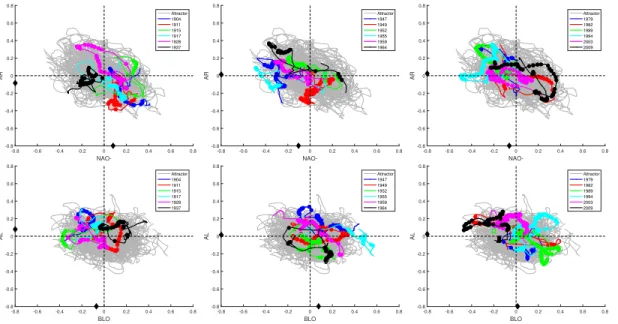
• Figure S6: Dynamical representation of the warmest summers for ERA20C during 1900-2010 in regimes AR-NAO- and BLO-AL.
• Figure S7: Dominants weather regimes during Summer Heatwave events in
Western-Europe for three reanalysis products (20CR, ERA20C, NCEP). • Figure S8: SLP anomalies in heatwave events (20CRv2c EM) for each period, • Figure S9: Temperature (y-axis) vs numbers of days (x-axis) during each heatwave
event for the 20CR Ensemble Mean (1871-2011) weather regimes.
ref NCEP ERA1 ERA2 ERA3 EM1 EM2 EM3 0.5 1.0 1.5 2.0 NAO−
ref NCEP ERA1 ERA2 ERA3 EM1 EM2 EM3
0.5
1.0
1.5
2.0
AR
ref NCEP ERA1 ERA2 ERA3 EM1 EM2 EM3
0.5
1.0
1.5
2.0
BLO
ref NCEP ERA1 ERA2 ERA3 EM1 EM2 EM3
0.5
1.0
1.5
2.0
AL
Figure S 1. Boxplots of Absolute Root Mean Square Error by period and weather regime. Colors represent each weather regime. (See also Table S1).
1950 1960 1970 1980 1990 2000 2010 −0.3 −0.1 0.1 0.3 NCEP anom.NA O − a 1900 1920 1940 1960 1980 2000 −0.3 −0.1 0.1 0.3 ERA20C anom.NA O − e 1950 1960 1970 1980 1990 2000 2010 −0.3 −0.1 0.1 0.3 NCEP anom.AR b 1900 1920 1940 1960 1980 2000 −0.3 −0.1 0.1 0.3 ERA20C anom.AR f 1950 1960 1970 1980 1990 2000 2010 −0.3 −0.1 0.1 0.3 NCEP anom.BLO c 1900 1920 1940 1960 1980 2000 −0.3 −0.1 0.1 0.3 ERA20C anom.BLO g 1950 1960 1970 1980 1990 2000 2010 −0.3 −0.1 0.1 0.3 NCEP anom.AL d 1900 1920 1940 1960 1980 2000 −0.3 −0.1 0.1 0.3 ERA20C anom.AL h 20CR ERA20C NCEP 1870 1880 1890 1900 1910 1920 1930 1940 1950 1960 1970 1980 1990 2000 2010 years Dominant WR NAO− AR BLO AL i
Figure S 2. Relative long-term summer weather regime frequency over the North-Atlantic region and their dominance in warmest summers in Western-Europe (1871-2016) using three reanalysis products (20CR, ERA20C, NCEP). As in figure S1, relative frequency of Summer SLP (hPa anomalies) weather regimes: NAO- (a,e), AR ( b,f ), BLO (c,g) and AL (d,h), but considering NCEP data (a-d,) and ERA20C (e-h). e, Warmest summers from 1871 to 2015 in Western-Europe with their dominant weather regime. Years are shown in x axis while y axis display each of the reanalysis products (20CR, ERA20C, NCEP). Circle size depends on temperature anomalies, the largest the warmest. Colors (black, red, green, blue) represents the dominant weather regime (NAO-, AR, BLO, AL) for each summer. The number of warmest summers are ponderate with the length of each dataset.
−10 0 10 20 30 40 45 50 55 60 Longitude Latitude a 20CR 2003 −10 0 10 20 30 40 45 50 55 60 Longitude Latitude d 20CR 1994 −10 0 10 20 30 40 45 50 55 60 Longitude Latitude g 20CR 1955 −10 0 10 20 30 40 45 50 55 60 Latitude j 20CR 1872 −10 0 10 20 30 40 45 50 55 60 Longitude Latitude b ERA20C 2003 −10 0 10 20 30 40 45 50 55 60 Longitude Latitude e ERA20C 1904 −10 0 10 20 30 40 45 50 55 60 Longitude Latitude h ERA20C 1955 −10 0 10 20 30 40 45 50 55 60 Latitude k ERA20C 1949 −10 0 10 20 30 40 45 50 55 60 Longitude Latitude c NCEP 2003 −10 0 10 20 30 40 45 50 55 60 Longitude Latitude f NCEP 1994 −10 0 10 20 30 40 45 50 55 60 Longitude Latitude i NCEP 1955 −10 0 10 20 30 40 45 50 55 60 Latitude −3 −2 −1 0 1 2 3 l NCEP 2015
Figure S 3. Temperature anomalies maps for warmest summers in Western-Europe. Each row correspond to a different dominant weather regime for some explanatory summers. Each column is a different reanalysis product.a-c, Summer 2003, where AL was the dominant weather regime. d-f, Summer of 1994, where AR was the dominant weather regime (Same frequencies of BLO and AR for NCEP during this summer). g-i, Summer of 1955, where BLO was the dominant weather regime. j-l, Since there is not a common summer for all the reanalysis datasets with NAO-as a dominant weather regime, here we show the most warmest summer (1872, 1904, 2015) where NAO- was the dominant weather regime in each reanalysis dataset (20CR, ERA20C, NCEP).
Figure S 4. 30yr-running correlations of summer mean temperatures and weather regime frequency in Western Europe. The data used is the Ensemble Mean of 20CRv2c. Warmest summers are marked with a vertical dashed line.Colors represents the weather regimes
17 18 19 20 21 22 23 24 1870 1880 1890 1900 1910 1920 1930 1940 1950 1960 1970 1980 1990 2000 2010 20CR a 17 18 19 20 21 22 23 24 1870 1880 1890 1900 1910 1920 1930 1940 1950 1960 1970 1980 1990 2000 2010 T emperature ERA20C b 17 18 19 20 21 22 23 24 1870 1880 1890 1900 1910 1920 1930 1940 1950 1960 1970 1980 1990 2000 2010 Years NCEP c
Figure S 5. Summer average temperatures (◦C) for Western-Europe. a, 20CR b, ERA20C and c, NCEP).
NAO--0.8 -0.6 -0.4 -0.2 0 0.2 0.4 0.6 0.8 AR -0.8 -0.6 -0.4 -0.2 0 0.2 0.4 0.6 0.8 Attractor 1904 1911 1915 1917 1928 1937 NAO--0.8 -0.6 -0.4 -0.2 0 0.2 0.4 0.6 0.8 AR -0.8 -0.6 -0.4 -0.2 0 0.2 0.4 0.6 0.8 Attractor 1947 1949 1952 1955 1959 1964 NAO--0.8 -0.6 -0.4 -0.2 0 0.2 0.4 0.6 0.8 AR -0.8 -0.6 -0.4 -0.2 0 0.2 0.4 0.6 0.8 Attractor 1979 1982 1989 1994 2003 2009 BLO -0.8 -0.6 -0.4 -0.2 0 0.2 0.4 0.6 0.8 AL -0.8 -0.6 -0.4 -0.2 0 0.2 0.4 0.6 0.8 Attractor 1904 1911 1915 1917 1928 1937 BLO -0.8 -0.6 -0.4 -0.2 0 0.2 0.4 0.6 0.8 AL -0.8 -0.6 -0.4 -0.2 0 0.2 0.4 0.6 0.8 Attractor 1947 1949 1952 1955 1959 1964 BLO -0.8 -0.6 -0.4 -0.2 0 0.2 0.4 0.6 0.8 AL -0.8 -0.6 -0.4 -0.2 0 0.2 0.4 0.6 0.8 Attractor 1979 1982 1989 1994 2003 2009
Figure S 6. Dynamical representation of the warmest summers (same as fig.3 in main text) for ERA20C during 1900-2010. Correlations of daily SLP fields and NAO- (x-axis), AR (y-axis) weather regimes in upper panels and correlations of daily SLP fields and BLO (x-axis), AL (y-axis) weather regimes in the bottom panels for three different periods. Warmest summers are colored as in the legend, light grey lines represent all data. Big circles represent days with temperature above 85th percentile. Average correlations of warmest summers with respect to each weather regime (black circle on x-axis). A moving average filter of 30 days window was applied to the warmest summers for better representation.
***
*
*
*
*
*
*
*
*
*
°
°
°
°
°
°
°
NAO − (19%)*
**
*
*
*
*
*
*
*
*
* *
*
*
***
°
AR (19%)*
*
*
*
*
*
*
* *
*
*
* *
*
*
*
*
*
*
*
*
*
*
°
°°
°
° °
°°
°
°
°
°
°
BLO (35%)*
*
*
*
*
*
*
*
*
* *
*
**
*
*
*
*
**
°
° ° °°
°
°°
°°°
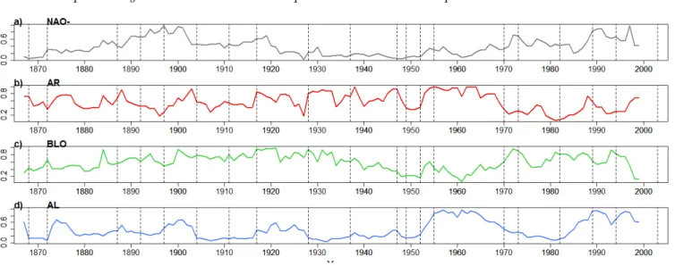
AL (26%) a b c d 17 18 19 20 21 22 23 24 25 26 27 28 29 30 17 18 19 20 21 22 23 24 25 26 27 28 29 30 1870 1890 1910 1930 1950 1970 1990 2010 1870 1890 1910 1930 1950 1970 1990 2010 years T emperature Dominant WR NAO − AR BLO AL N. of days 5 15Figure S 7. Dominant weather regimes during Summer Heatwave events in Western-Europe. Summer heatwave events (P90th Percentile) from 1871 to 2015 for different reanalysis products: 20CR (circle with stars), ERA20C (empty circle), and NCEP (circles with inner circle). Colors correspond to the dominant Weather regime (a-d,) in each event, temperature (y-axis) and years (x-axis). Circle sizes depend on the event duration by number of days, the larger the longer duration. Percentages show the frequency of each weather regime. Linear fits are shown in black solid lines.
Figure S 8. mean SLP anomalies in heatwave events (20CRv2c EM) for each period. As figure 6, a-d show mean SLP anomalies in heatwaves events for each group of years. Numbers at the top right corner represent the number of heatwave events during that period in comparison with the total number of heatwave events in 20CRv2c EM. Mean SLP anomalies in heatwaves events pre-1930 and post-1930 are represented in e-f, respectively.
Figure S 9. Density plot of heatwave events. Temperature (y-axis) vs numbers of days (x-axis) during each heatwave event for the 20CR Ensemble Mean (1871-2011) weather regimes. Colors represent the number of hetwaves events.
AbsRM SE Period NAO- AR BLO AL (1970-2010) 1.01 1.00 0.98 0.99 NCEP (1948-2015) 1.01 1.0 1.01 1.00 (1900-1936) 0.95 0.99 0.96 0.97 ERA 20C (1937-1973) 1.03 0.99 1.01 1.01 (1974-2010) 1.03 1.01 1.03 1.03 (1871-1917) 0.94 1.01 1.00 0.99 20CR (1918-1964) 1.03 0.98 1.02 1.01 (1965-2011) 1.04 1.01 0.99 1.01
Table S 1. Absolute error of the Root mean square deviation (AbsRM SE)
of the truncated EOFs during the training period( NCEP:1970-2010) by Weather Regimes during summer in Western-Europe (see also Figure S1)