Will GDP growth increase happiness in developing countries?

HAL Id: halshs-00564985

https://halshs.archives-ouvertes.fr/halshs-00564985v2

HAL is a multi-disciplinary open access

archive for the deposit and dissemination of sci-entific research documents, whether they are pub-lished or not. The documents may come from teaching and research institutions in France or abroad, or from public or private research centers.

L’archive ouverte pluridisciplinaire HAL, est destinée au dépôt et à la diffusion de documents scientifiques de niveau recherche, publiés ou non, émanant des établissements d’enseignement et de recherche français ou étrangers, des laboratoires publics ou privés.

Will GDP growth increase happiness in developing

countries?

Andrew E. Clark, Claudia Senik

To cite this version:

Andrew E. Clark, Claudia Senik. Will GDP growth increase happiness in developing countries?. 2010. �halshs-00564985v2�

WORKING PAPER N° 2010 - 43

Will GDP growth increase happiness

in developing countries?

Andrew E. Clark Claudia Senik

JEL Codes: D63, I3, O1

Keywords: Income, subjective well-being, comparisons, adaptation, development

P

-

S

E

48,BD JOURDAN –E.N.S.–75014PARIS TÉL. :33(0)143136300 – FAX :33(0)143136310

Will GDP Growth Increase Happiness in Developing Countries?

Andrew E. Clark and Claudia Senik∗

March 20th 2011

Summary

This paper asks what low-income countries can expect from growth in terms of happiness. It interprets the set of available international evidence pertaining to the relationship between income growth and subjective well-being. Consistent with the Easterlin paradox, higher income is always associated with higher happiness scores, except in one case: whether growth in national income yields higher well-being is still hotly debated. The key question is whether the correlation coefficient is “too small to matter”.

The explanations for the small correlation between national income growth and subjective well-being over time appeal to the nature of growth itself (from negative side-effects, such as pollution), and to the psychological importance of relative concerns and adaptation. The available evidence contains two important lessons: income comparisons do seem to affect subjective well-being. even in very poor countries; however, adaptation may be more of a rich-country phenomenon.

Our stand is that the idea that growth will increase happiness in low-income countries cannot be rejected on the basis of the available evidence. First, cross-country time-series analyses are based on aggregate measures, which are less reliable than those at the individual level. Second, development is a qualitative process involving take-off points and thresholds. Such regime changes are visible to the eye through the lens of subjective satisfaction measures. The case of Transition countries is particularly impressive in this respect: average life satisfaction scores closely mirrored changes in GDP for about the first ten years of the transition process, until the regime became more stable. The greater availability of subjective measures of well-being in low-income countries would greatly help in the measurement and monitoring of the different stages and dimensions of the development process.

∗ Paris School of Economics, 48 Boulevard Jourdan, 75014 Paris, France. E-mail addresses: [email protected], [email protected]. We thank Hélène Blake for precious research assistance and CEPREMAP for financial support. We are very grateful to Emmanuel Commolet, Nicolas Gury and Oliver Charnoz for incisive comments on a previous draft, and Alpaslan Akay, Alexandru Cojocaru, Luca Corazzini, Ada Ferrer-i-Carbonell, Armin Falk, Carol Graham, Olof Johansson-Stenman, John Knight, Andrew Oswald, Bernard Van Praag, Mariano

I. INTRODUCTION ... 4  

I.1 The data used in the paper... 5  

I.2 Subjective well-being measures: why use them and are they reliable? ... 6  

I. THE PARADOXICAL RELATIONSHIP BETWEEN GROWTH AND WELL-BEING ... 11  

I.1. Income raises happiness in the cross section ... 11  

a.   Within-country cross-section ... 11  

b.   Cross-sections of countries ... 12  

c.   A positive relation in individual panel data ... 14  

I.2. The diminishing returns to income growth ... 15  

a.   Is there a threshold in the utility of growth? ... 15  

b.   But the happiness-log GDP per capita gradient does not tend to zero. ... 16  

1.3 “Rather than diminishing marginal utility of income, there is a zero marginal utility of income” ... 17  

I.4   Is the time-series correlation small enough to ignore? ... 19  

A note on statistical power ... 20  

I.5 Subjective well-being and the business cycle... 21  

II. EXPLANATIONS RELATED TO GROWTH ITSELF: CHANNELS AND NEGATIVE SIDE-EFFECTS ... 23  

II.1 Quality of Life: channels from GDP growth to happiness ... 23  

a. Cross-section correlation between GDP growth and Quality of Life indicators ... 24  

b. Time-series correlation between GDP growth and Quality of Life indicators... 25  

II. 2. Negative side-effects of growth... 26  

III.   EXPLANATIONS RELATED TO THE HAPPINESS FUNCTION ITSELF (HUMAN BEINGS ARE SOCIAL ANIMALS)... 27  

III.1. Income comparisons ... 27  

c. Absolute versus relative poverty... 35  

III.2. Adaptation ... 37  

a. Evidence in Developed Countries... 38  

b.   Evidence in LDCs... 39  

III.3 Bounded scales: What exactly is relative?... 41  

IV.   CONCLUSIONS AND TAKE-HOME MESSAGES: HOW CAN WE USE SUBJECTIVE VARIABLES IN ORDER TO UNDERSTAND THE GDP-HAPPINESS RELATIONSHIP?... 42  

I. I

Is income growth the only thing that matters in development, and does it raise the level of well-being of the population? De facto, economic development is generally identified with growth in GDP per capita: International organizations, such as the United Nations Organization, the OECD, the World Bank and the International Monetary Fund, classify countries as developed, intermediate or low-development, depending on whether they are

above or below certain thresholds of GDP per capita. However, development is of course

more than just income growth. It is a multi-dimensional process, which involves not only a quantitative increase in capital accumulation, production and consumption, but also qualitative social and political changes that enlarge the choice set of the individuals concerned. Institutional progress, human rights, democracy, gender equality and other capacities are an integral part of development. We can then ask whether these qualitative objectives can be attained by maximizing GDP. And in addition, we might worry that income growth will yield negative side-effects, which reduce well-being, such as environmental externalities, the destruction of traditional social links, the concentration of the population in urban and suburban centres, the development of work-related stress, and so on.

“Is growth obsolete?” The provocative title of the paper by William Nordhaus and James Tobin (1973) reflects the radical questioning of growth as an engine of well-being. Although the authors answer this question in the negative, many economists and social scientists have come to the conclusion that, in developed countries, economic growth per se has little impact on well-being and should therefore not be the primary goal of economic policy (see Oswald, 1997). How much of this argument can we extend to developing countries? Or should we follow the proposition of Inglehart et al. (2008) that material growth, as measured by GDP per capita, is welfare-improving in developing countries, as it takes people out of poverty and precarity, but that it is useless in modern and “post-modern” societies where survival is taken for granted and human development becomes the only valuable goal?

This paper will address the relationship between GDP growth and well-being in developing countries through the lens of subjective well-being measures, i.e. self-declared satisfaction

the world. Using these measures as a shortcut to people’s well-being, we will try to see whether GDP growth is really a proxy for and a valuable route to happiness.

One of the most important but equally most controversial issues in the subjective well-being literature is precisely the income-happiness relationship. In a famous article, Easterlin (1974) ironically asked whether “raising the incomes of all will raise the happiness of all?” This was based on the observation that average happiness measures remained flat over the long-run in countries which had experienced high rates of GDP growth. The income-happiness nexus has been vividly debated for the past two decades by economists, psychologists and political scientists. However, most of the evidence to date on the relationship between income and subjective well-being is based on developed countries. Is the Easterlin paradox also valid for developing countries, or is it a rich country phenomenon?

This paper presents an overview of the evidence that has accumulated during the past twenty years of research and illustrates some of the findings using a widely used international database (the World Values Survey, 1981-2005) containing individual life satisfaction and happiness information. In a first section, we present the relationship between income, income growth and subjective well-being and ask to what extent the patterns usually observed in developed countries also hold in developing countries. We discuss the potential existence of a threshold effect in the welfare returns of growth, where the latter are higher in low- as opposed to high-income countries. Sections 2 and 3 then present the classic explanations of the Easterlin paradox and their relevance to developing countries. Here, we distinguish the positive and negative side-effects of growth, and the limits to the way in which income can produce subjective well-being that stem from human nature itself (comparison and adaptation effects). Finally, we provide some reasons why we believe that cross-section and panel analysis based on individual data is more reliable than that using aggregated times-series. Accordingly, we conclude that the positive income-well-being gradient, supported by individual and cross-sectional data, is difficult to dismiss.

I.1 The data used in the paper

This paper essentially hinges on results in the existing literature. However, we have added a number of figures of our own, using the five waves of the well-known World Values Survey (WVS, 1981-2008) database covering 105 countries, including high-income, low-income and Transition countries, which account for 90% of the world’s population. Happiness measures

were mostly taken from the WVS and the European Social Survey (ESS): this is the case for 250 out of 368 observations. When happiness data was missing, we used information from the ISSP (101 observations) and 17 observations from the 2002 Latinobarometer. All of these

datasets are available at http://worldvaluessurvey.org. The happiness and life satisfaction

questions were administered in the same format in all these surveys, with equivalent translations for all countries. The wording of the Happiness question was: “If you were to

consider your life in general these days, how happy or unhappy would you say you are, on the whole?: 1. Not at all happy; 2. Not very happy; 3. Fairly happy; 4. Very happy”. In the WVS,

the wording of the Life Satisfaction question was: “All things considered, how satisfied are

you with your life as a whole these days?: 1(dissatisfied) … 10 (very satisfied)”. The surveys

cover representative samples of the population of participating countries, with an average sample size of 1400 respondents at each wave. We calculated the national average value of the answers to each of these questions (treating them as continuous variables). We also created a misery index defined as the percentage of people who declare themselves to be very happy, or very satisfied, minus the percentage of respondents declaring themselves to be not at all happy, or not at all satisfied. As the results from the two aggregate well-being measures were very similar, we only present here the Figures based on average well-being.

The paper also appeals to a measure of trust, which is available in the WVS: “Generally

speaking, would you say that most people can be trusted or that you can’t be too careful in dealing with people?: 1. Most people can be trusted; 0 . Can't be too careful”. The GDP per

capita and annual GDP growth information comes from Heston, Summers and Aten – the Penn World Table. We also use other quantitative indicators which are available in the World databank, such as the Gini measure of income inequality, women’s fertility rates, adult

literacy rates, and life expectancy at birth (see http://data.worldbank.org/). The qualitative

indicators of governance were taken from Freedom House and Polity IV

(http://www.qog.pol.gu.se/, http://www.freedomhouse.org, http://www.govindicators.org, and

http://www.systemicpeace.org/polity/polity4.htm ). All these data are available from the

World Data Bank: http://www.worldvaluessurvey.org.

I.2 Subjective well-being measures: why use them and are they reliable?

The critical quality of subjective well-being is that it is self-reported. Instead of a third person designing some set of criteria (income, health, education, housing etc.) which will define how

of the quality of their life. While some have doubted the usefulness of subjective measures, we think that there are fairly compelling reasons to include them in the Economists’ arsenal. Think of an individual’s level of well-being as being some appropriately-weighted sum of all of the aspects of life that matter to her. There are at least two significant obstacles for it to be measured objectively. The first is that we need to be sure that we cover all of the aspects of life that are important to the individual, and it seems a priori difficult to make up a definitive measurable list of these. The second problem is that we have to apply appropriate weights to construct the final well-being index. This might appear problematic right from the start: in the context of the aggregate data used in the Human Development Index, for example, how much is literacy worth in terms of life expectancy? Moreover, it would appear extremely likely that any such weighting will differ between individuals, and probably in ways that it is not easy to observe. It is consequently very tempting to sidestep the difficulties involved by asking individuals to make these calculations themselves, in responding to evaluative questions about their own lives.

The well-being questions asked in this context are often very simple ones, such as “How

dissatisfied or satisfied are you with your life overall?” (from the British Household Panel

Survey), which is answered on a seven-point scale, with one referring to “Not satisfied at all”, four to “Neither satisfied nor dissatisfied” and seven to “Completely satisfied”. Alternatively individuals may be asked about their happiness, as in the following question from the American General Social Survey (GSS): “Taken all together, how would you say things are

these days, would you say that you are very happy, pretty happy, or not too happy?” Other

questions may refer to positive and negative affect or mental health.

These questions are increasingly widely included in surveys across the social sciences. One reason for their popularity is that they are simple to put into questionnaires, as probably the majority of those that appear are single-item (although there are very many multiple-item

scales that are also available in the literature: see

http://acqol.deakin.edu.au/instruments/instrument.php for a summary of some of these). A

second point is that the vast majority of respondents seem to understand the question: non-response rates are very low. The third reason, which from our point of view is the most important, is that the answers to these questions do seem to pick up how well people are doing.

This last statement might seem to be rather uncontroversial: after all, we would expect a question on life satisfaction to measure exactly that. The potential problem lies exactly in the subjectivity of the reply. In particular, if individuals understand the question differently, or use the response scales differently, then there is a danger that someone who answers six on a one to seven satisfaction scale is no better off than another person who has given an answer of five. Luckily there is by now a varied body of evidence suggesting that these subjective well-being measures do contain valid information.

A first point to make is that subjective well-being measures are well-behaved, in the sense that many of the correlations make sense. In cross-section data, variables reflecting marriage, divorce, unemployment, birth of first child and so on are typically correlated with individuals’

subjective well-being in the expected direction.1 If the answers to well-being questions were

truly random, then no such relationship would be found.

We want to know whether asking A how happy she is will provide information about her unobserved real level of happiness. One simple check, called Cross-Rater Validity, is to ask B whether she thinks A is happy. This work has been carried out in a number of settings (see Sandvik et al., 1993, and Diener and Lucas, 1999), including asking friends and family, or the person who administered the interview. Alternatively, we can use individuals who do not know the subject: B may be shown a video recording of A, or may read a transcription of an open-ended interview with A. In all cases, B’s evaluation of the respondent’s well-being matches well with the respondent’s own reply.

Another approach to validation consists in relating well-being scores to various physiological and neurological measures. It has been shown that answers to well-being questions are correlated with facial expressions, such as smiling and frowning, as well as heart rate and blood pressure. The medical literature has shown that well being scores are correlated with

digestive disorders and headaches, coronary heart disease and strokes. Research has also

looked at physical measures of brain activity. Particular interest has been shown in the differences in brain wave activity between the left and right prefrontal cortexes, where the former is associated with positive and the latter with negative feelings. These differences can

well-be measured using electrodes on the scalp or scanners. Research has shown (for example, Urry et al., 2004) that these differences in brain activity are correlated with individual

well-being responses. These measures of brain asymmetry have been shown to be associated with

cortisol and corticotropin releasing hormone (CRH), which regulate the response to stress, and antibody production in response to influenza vaccine (Davidson, 2004). Consistent with subjective well-being and brain asymmetry measuring the same underlying construct, individuals reporting higher life satisfaction scores were less likely to catch a cold when exposed to a cold virus, and recovered faster if they did (Cohen et al., 2003).

The last block of evidence that people “mean what they say” is that, in data following the same individual over a long period of time, those who say that they are dissatisfied with a certain situation are more likely to take observable action to leave it. This phenomenon is apparent in the labor market, where the job satisfaction that the individual reports at a certain point in time is a good predictor of her being observed in the future to have quit her job (examples are Freeman, 1978, Clark et al., 1998, Clark, 2001, and Kristensen and Westergaard-Nielsen, 2006). One important subsidiary finding in this literature is the job satisfaction predicts quits even when we take into account the individual’s wages and hours of work. This prediction of future behavior seems to work for the unemployed as well as for the employed. Clark (2003) shows that mental stress scores on entering unemployment in BHPS data predict the length of the unemployment spell, with those who suffered the sharpest drop in well-being upon entering unemployment having the shortest spell. This finding has been replicated in using the life satisfaction scores in GSOEP data by Clark et al., 2010). Outside of the labor market, well-being scores have been

shown to predict the length of life (Palmore, 1969, Danner et al., 2001). Satisfaction measures

have also recently been shown to predict future marital break-up (Gardner and Oswald, 2006,

Guven et al., 2010).

One potential use of the analysis of subjective well-being is that it arguably provides us with information on trade-offs between different aspects of an individual’s life. If one extra hour of work per week has the same effect on well-being as does 80 Euros in additional earnings per month, then the shadow wage (the wage that would compensate for one extra hour of work) is around 18 Euros and 50 cents per hour. Some of examples of these well-being trade-offs have appeared in the recent literature. For example, Blanchflower and Oswald (2004, p 1381), using American and British data, came to the conclusion that: “To compensate men for

annum. A lasting marriage is worth 100000$ per annum (when compared to widowhood or separated)”.

This capacity of subjective data to weight the different dimensions of development one against the other (to calculate marginal rates of substitution between two dimensions) is particularly adapted to the multidimensionality of economic development. The structure of the well-being equation, as estimated in a country, can be seen as a synthetic measure that would have aggregated the different arguments of a social welfare function. The usual problem of the social planner (and of the social choice school of normative economics) is indeed to decide on the weights that should be attached to the different arguments of the social objective function. Subjective measures allow avoiding this obstacle by measuring directly the synthetic result of the weighting alchemy made by individuals themselves. An illustration of this is the paper by Di Tella and MacCulloch (2008, pp.31-33), where the authors use the American GSS and the Eurobarometer to estimate national welfare functions. They propose such marginal rates of substitution:

- Life expectancy / income: “A person who expects to live one year longer due to the

reduction in the risk of death is willing to pay $5052 in annual income in exchange (6.6% of GDP per capita)”.

- Life expectancy / unemployment: “In terms of the unemployment rate, denying an

individual one year of life expectancy has an equivalent cost to increasing the unemployment rate by 1.1 percentage point”.

- Pollution/GDP: “a one standard deviation increase in SOx emissions, equal to a rise

in 23kg per capita, has a decrease on well-being equivalent to a 15% drop in the level of GDP per capita.”

- Inflation/unemployment: “a 1% point rise in the level of inflation reduces happiness

by as much as a 0.3 percentage point increase in the unemployment rate”.

- Crime/GDP: “a rise in violent crime from 242 to 388 assaults per 100000 people in

the United States (i.e. a 60% rise) … would be equivalent to a drop of approximately 3.5% in GDP per capita”.

These examples illustrate the capacity of subjective well-being measures to serve as a useful tool for public policy aimed at maximizing well-being as countries develop.

Before we turn to the evidence on growth and subjective well-being, we should warn the reader of two abusive approximations contained this paper. First, we use the terms happiness, life satisfaction and well-being indiscriminately. Second, we treat these measures as though they were cardinal, although they are more properly ordinal. In doing so, as do the bulk of economists working on happiness measures, we follow the route opened by Ferrer-i-Carbonnell and Frijters (2004).

I.

G

One of the main catalysts in the voluminous and rapidly expanding literature on income and happiness has been Easterlin’s seminal article (1974; updated in 1995), setting out the ‘paradox’ of substantial real income growth in Western countries over the last fifty years, but without any corresponding rise in reported happiness levels. This finding is paradoxical for a number of reasons. First it runs counter to the popular prior that increased material wealth and greater freedom of choice should go hand-in-hand with higher well-being. In a way, our societies are organized on this implicit principle. Second, it seems to contradict a large body of scientific empirical evidence based on cross-sections of countries, and on within-country individual panel data. This section presents and discusses the available evidence on these contradictory findings, and asks whether the Easterlin paradox is a rich-country phenomenon or also something relevant for policy-makers in developing countries. A summary of the wide-ranging data sources and results appears in Appendix A.

I.1. Income raises happiness in the cross section a. Within-country cross-section

“As far as I am aware, in every representative national survey ever done, a significant

bivariate relationship between happiness and income has been found” (Easterlin 2005, p. 67).

Almost all of the empirical work based on within-country surveys include individual income or household income (or more precisely, the log of income) as a control variable to explain well-being. Log income invariably attracts a positive and statistically significant coefficient,

of considerable size. It is typically one of the most important correlates of self-declared happiness. “When we plot average happiness versus average income for clusters of people in

a given country at a given time…rich people are in fact a lot happier than poor people. It’s actually an astonishingly large difference. There’s no one single change you can imagine that would make your life improve on the happiness scale as much as to move from the bottom 5 percent on the income scale to the top 5 percent” (Frank, 2005, p. 67). This holds for both

developed and developing countries, even if it has sometimes been suggested that the income-happiness slope is larger in developing or transition than in developed economies (see Clark et al., 2008, for a survey).

Layard et al. (2010) for instance, report that within a country, a unit rise in log income raises individual self-declared happiness by 0.6 units on average (on a 10-point scale). Stevenson and Wolfers (2008, p. 13) estimate the within-country well-being-income gradient over each of the countries available in a number of international datasets (the American General Social Survey, the World Values Survey, the Gallup World Poll, etc.). They conclude that: “Overall,

the average well-being-income gradient is 0.38, with the majority of the estimates between .25 and .45 and 90 percent are between 0.07 and 0.72. In turn, much of the heterogeneity likely reflects simple sampling variation: the average country-specific standard error is 0.07, and 90 percent of the country-specific regressions have standard errors between 0.04 and 0.11”.

As an illustration, Figure 1.A depicts the household income-happiness gradient in the United States. The fitted relationship is well-described by a log-linear function. The same findings hold in a series of surveys covering developing countries. Figure 1.B shows the income decile-happiness gradient in China in 2007 (based on World Values Survey data): the same positive relationship appears. In general, the fact that in a given society the rich are happier than the poor is a well-established and undisputed empirical finding in this literature.

b. Cross-sections of countries

The empirical evidence is even more conclusive and consensual regarding the income-happiness gradient across countries. Deaton (2008), for example, finds an elasticity of 0.84 between log average income and average national satisfaction across a large set of nationally representative samples of individuals living in 129 developed and developing countries, collected by the 2006 Gallup World Poll. In the same spirit, Inglehart (1990, chapter 1) analyzes data from 24 countries at different levels of development and finds a 0.67 correlation

between GNP per capita and life satisfaction. In a more recent paper, Inglehart et al. (2008) report a correlation of 0.62 using all available waves of the World Values Survey. Wolfers and Stevenson (2008, p. 12), using a very comprehensive set of data, uncover “a

between-country well-being-GDP gradient [..] typically centered around 0.4”.2 In the surveys analyzed by Inglehart et al. (2008), 52% of the Danes indicated that they were very satisfied with their life (with a score of over 8 on a 10-point scale) and 45% said they were very happy. On the contrary, in Armenia only 5% said they were very satisfied and 6% very happy.

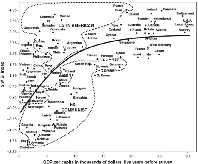
Figure 2.A (taken from Inglehart et al., 2008) shows the concave relationship between income per capita and average happiness across developed, developing and Transition countries of the world, over the 1995-2007 period. A similar graph appears in Deaton (2008) based on the World Values Survey (1996) and the Gallup World Poll (2006), which we reproduce here as Figure 2.B. As shown in Figure 2.C, “Each Doubling of GDP is Associated with a Constant

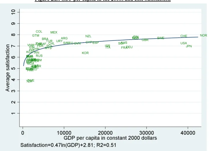
Increase in Life Satisfaction” across countries (Deaton, 2008). Figure 2.D illustrates the good

fit of a log-linear relationship between income per capita and average life satisfaction across countries of the world, in the late 2000s, using the most recent waves of the World Values Survey.

Many other contributions to the “macroeconomics of happiness” have documented the fact that individuals in general report higher happiness and life satisfaction scores in higher-income countries (see for example Blanchflower, 2008), even if certain types of societies seem to be more conducive to happiness than others (Inglehart et al., 2008). In Figure 2.A, for example, Latin American countries are systematically found above the regression line, while Transition countries form a cluster lying below the regression line tracing out the average

relationship in the data.3

2 _{These estimate vary because of the composition of the sample and the controls included in the regressions.} 3 _{According to Guriev and Zhuravskaya (2009), the reasons for the lower happiness level in Transition countries} are the deterioration in public goods provision, the increase in macroeconomic volatility and mismatch of human

Development and the inequality of subjective well-being

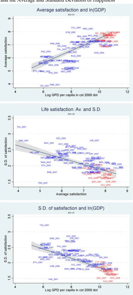
As a complement to the average income - average happiness relationship, we have also looked at the relation between average life satisfaction scores and their standard deviation (treating well-being as a continuous variable). Cross-country analysis produces a striking observation: the higher is average national happiness, the lower is the within-country standard deviation of happiness. As such, richer countries have both higher average scores and lower standard deviations of life satisfaction (Figure 6). This suggests one potentially important benefit of GDP growth for low-income countries. If individuals are risk-averse, reducing the variance of SWB in a given society is a valuable objective of public policy.

c. A positive relation in individual panel data

Thanks to the increased availability of population panel surveys in a number of different countries, a variety of analyses of individual well-being have been able to control for unobserved individual fixed effects, such as personality traits. All of this work has concluded that there is a positive correlation between the change in real income and the change in happiness (see, for example, Winkelmann and Winkelmann, 1998, Ravallion and Lokshin, 2002, Ferrer-i-Carbonell and Frijters, 2004, Senik, 2004 and 2008, Ferrer-i-Carbonell, 2005, and Clark et al., 2005). Further, a number of these articles have appealed to exogenous variations in income in order to establish more firmly the causal effect of individual income on happiness (e.g. Gardner and Oswald, 2007, Frijters et al., 2004a, 2004b and 2006, and Pischke, 2010). The slope of the income-happiness relationship is not necessarily the same between groups (Clark et al., 2005, Frijters et al., 2004a, and Lelkes, 2006). The coefficient on the within-individual change in log income is typically found to be in the vicinity of 0.3 (Layard et al., 2010, and Senik 2005).

There is thus both single-country and international evidence showing that the rich are happier than the poor within a given country, that those in richer countries are on average happier than those in poorer countries, and that an increase in individual income over time is associated with increasing happiness. At this stage then, the evidence is strongly in favour of a development policy based on GDP growth in low-income countries.

I.2. The diminishing returns to income growth

The situation is not completely clear-cut, however, as illustrated by the panels of Figures 1 and 2: the positive relationship between income and happiness exhibits diminishing returns. This comes as no surprise to economists, who are accustomed to the idea of the concavity of preferences, i.e. decreasing marginal utility and risk-aversion. Concretely, this means that the effect of earning an additional ten thousand dollars on subjective well-being becomes progressively smaller as one’s initial level of income increases. This is consistent with the good fit of the log functional form for income-happiness relationship, which is a familiar result in the empirical analysis of subjective well-being across the social sciences.

a. Is there a threshold in the utility of growth?

“Once a country has over $15,000 per head, its level of happiness appears to be independent

of its income per head” (Layard, 2003, p. 17)

Many authors have suggested a threshold in the welfare effect of income. They recognize that rich countries are happier than poor countries, but believe that there is no strong relationship between GDP per capita and happiness among rich countries. This threshold separates “survival societies” and “modern societies” (Inglehart et al., 2009). It is usually found to be in

an interval from US$10,000 to $15000 per annum (Di Tella et al., 2007).4 Layard (2005, p.

149) thus writes: “if we compare countries, there is no evidence that richer countries are

happier than poorer ones—so long as we confine ourselves to countries with incomes over $15,000 per head.… At income levels below $15,000 per head things are different….”. Frey

and Stutzer (2002, p. 416) similarly claim that “income provides happiness at low levels of

development but once a threshold (around $10,000) is reached, the average income level in a country has little effect on average subjective well-being”.

4 _{This notion of a satiation point also goes back to Adam Smith’s concept of “a full complement of riches”,} beyond which there could be not be desire for more money. The large landholders of the 18th _{Century had} (according to him) reached this limit. However, there may be a limit to the quantity of wealth someone can enjoy in a given society at a certain point of time, but this does not mean that this limit cannot be stretched by the set of new choices brought about by economic growth (e.g. the internet). In other words, the “full complement of riches” could be wider in richer than in less-developed countries.

Even more explicitly, Inglehart (1997, pp. 64-65) concludes that: “the transition from a

society of starvation to a society of security brings a dramatic increase in subjective well-being. But we find a threshold at which economic growth no longer seems to increase subjective well being significantly. This may be linked with the fact that, at this level, starvation is no longer a real concern for most people. Survival begins to be taken for granted […] At low levels of economic development, even modest economic gains bring a high return in terms of caloric intake, clothing, shelter, medical care and ultimately in life expectancy itself. […]. But once a society has reached a certain threshold of development … one reaches a point at which further economic growth brings only minimal gains in both life expectancy and subjective well-being. There is still a good deal of cross national variation, but from this point on non-economic aspects of life become increasingly important influences on how long and how well people live”… The authors continue to reach the same conclusion with updated

data: “Happiness and life satisfaction rise steeply as one moves from subsistence-level poverty

to a modest level of economic security and then levels off. Among the richest societies, further increases in income are only weakly linked with higher levels of SWB” (Inglehart et al., 2008,

p. 268).

If true, the implication of these findings for developing countries is that GDP growth should be seen as a temporary objective, to be retained only up to a certain level.

b. But the happiness-log GDP per capita gradient does not tend to zero.

In spite of these strong claims, the cross-country evidence in favour of such a subsistence level is far from consensual. Bringing together a number of international survey datasets that covering about 90% of the world’s population, including many developing countries (based on the World Values Survey and the Gallup World Poll), Stevenson and Wolfers (2008, pp. 11-12) test for the idea of a cut-point at $15,000 per capita per annum (in constant 2000 dollars). They estimate the happiness-GDP per capita gradient, and find that: “the

well-being-GDP gradient is about twice as steep for poor countries as for rich countries. That is […] a rise in income of $100 is associated with a rise in well-being for poor countries that is about twice as large as for rich countries”. However, the marginal utility of GDP growth is still

positive in developed countries. “The point estimates are, on average, about three times as

large for those countries with incomes above $15,000 compared to those countries with incomes below $15,000”. […] Taken at face value, the Gallup results suggest that a 1 percent

being in rich as in poor nations. Of course, a 1 percent rise in U.S. GDP per capita is about ten times as large as a 1 percent rise in Jamaican GDP per capita”.

This result is consistent with Deaton’s analysis of the same Gallup World Poll data (Figure 2.B): “the relationship between log per capita income and life satisfaction is close to linear.

The coefficient is 0.838, with a small standard error. A quadratic term in the log of income has a positive coefficient: confirming that the slope is higher in the richer countries! […] Using 12000$ of income per capita as a threshold between rich and poor countries shows that the slope in the higher income countries is higher! […] If there is any evidence for a deviation, it is small and is probably in the direction of the slope being higher in the high-income countries”.

Deaton (2008) concludes that “the slope is steepest among the poorest countries, where the

income gains are associated with the largest increases in life satisfaction, but it remains positive and substantial even among the rich countries; it is not true that there is some critical level of GDP per capita above which income has no further effect on life satisfaction”. In

other words, there is indeed diminishing marginal utility to GDP growth, as the level of GDP

per capita increases, but the return to growth does not converge to zero.5

To summarize, an undisputed finding of the happiness literature based on cross-sections of countries is that the relationship between income per capita and happiness is concave, i.e. has diminishing returns. However, there is no consensus on the existence of a subsistence threshold beyond which the marginal utility of income falls to zero.

1.3 “Rather than diminishing marginal utility of income, there is a zero marginal utility of income”

The most powerful criticism of pro-growth policy hinges on the empirical evidence regarding the within-country long-run changes in GDP and happiness. Visual evidence provided by Easterlin and his co-authors (1974, 1995, 2005, 2007, 2009 and 2010) illustrates the flatness

5 _{It is worth underlying that while the log function is indeed concave, it is not bounded from above. If y=log(x),} then y does not tend to any fixed value as x tends to infinity. Yet, this is the message that a vast majority of specialists in the field have drawn from the decreasing marginal utility of income and the good fit of the log-linear functional form for the relationship between income and happiness.

of the long-run happiness curve plotted against time. One of the most famous and spectacular of these flat curves is show in Figure 3.A, taken from Easterlin and Angelescu (2007). In spite of the doubling of U.S. GDP per capita over a 30-year period (1972-2002), the average happiness of Americans has remained constant. Average happiness is calculated using repeated cross-sections from the American General Social Survey. The same type of pattern has been uncovered in a number of other contributions, with long time-series data covering different developed countries (see Diener and Oishi, 2000). The claim supported by these graphs is radical: in the words of Richard Easterlin, “Rather than diminishing marginal utility

of income, there is a zero marginal utility of income” (Easterlin and Angelescu, 2007, p. 8).

The absence of any long-run correlation between growth and happiness could be explained by the decreasing marginal utility of income uncovered in the cross-section. However, Easterlin strongly rejects this interpretation: “The usual constancy of subjective well-being in the face

of rising GDP per capita has typically been reconciled with the cross-sectional evidence on the grounds that the time series observations for developed nations correspond to the upper income range of the cross-sectional studies, where happiness changes little or not al all as real income rises.” But “the income change over time within the income range used in the point-of-time studies do not generate the change in happiness implied by the cross-sectional pattern”. (Easterlin and Angelescu, 2007, p. 24). For example: “in 1972, the cohort of 1941-1950 had a mean per capita income of about 12000$ (expressed in 1994 constant prices). By the year 2000, the cohort’s average income had more than doubled, rising to almost 27000$. According to the cross-sectional relation, this increase should have raised the cohort’s mean happiness from 2.17 to 2.27. In reality, the actual happiness of the cohort did not change”.

In some of his articles (Easterlin, 2005a, and Easterlin and Sawangfa 2005), Easterlin has forcefully underlined that cross-section evidence cannot be transposed to the relationship over time. The change in average self-reported happiness in a country, in the long-run, is not correctly predicted by the instantaneous cross-section relationship between income per head and happiness. Hence: “knowing the actual change over time in a country’s GDP per capita

and the multi-country cross-sectional relation of SWB to GDP per capita adds nothing, on average, to one’s ability to predict the actual time-series change in SWB in a country”

(Easterlin and Sawangfa, 2009, p. 179). This is illustrated in Figure 3.B, taken from Easterlin (2005a, p. 16), which contrasts the actual (flat) evolution of happiness in Japan, and the predicted (log-linear) change over time.

Hence, the positive concave relationship between GDP per capita and SWB, observed in the cross section, cannot be used to predict the change in SWB in developing countries over time. This new “no bridge” theory underlines the “fallacy” of transposing cross-sectional relations to time-series data. The lesson for developing countries is that they should not necessarily expect to reach the higher level of well-being that is typical of developed countries by growing over time.

I.4 Is the time-series correlation small enough to ignore?

In spite of the spectacular visual evidence offered by Easterlin, his rejection of any correlation between over time between growth and happiness is still the object of vivid controversy. In particular, one disputed point is whether the size of the correlation coefficient between SWB and GDP per capita is statistically significant, and large. It is small, but is it “small enough to

ignore”? (Hagerty and Veenhoven, 2000, p. 4).

For instance, the absence of correlation between growth and happiness in the fast-developing countries of Japan (after WWII) and China (after 1980) is particularly disappointing. However, Stevenson and Wolfers (2008) have noted a number of discontinuities in the wording of the happiness question and in the sampling of the Japanese cross-sections used by Easterlin. With respect to China, the evidence is scarce (only three points in time) and Hagerty and Veenhoven (2000) underline the fact that the Chinese sample is not representative of the population, as it was initially biased towards more urban demographic groups.

Other work on the long-run macroeconomic time series of happiness has concluded that there is a positive relationship between growth in GDP per capita and well-being. Exploiting the World Values Survey, Hagerty and Veenhoven (2003) found that GDP is positively related to the number of “happy life years” in 14 of the 21 countries available in the dataset. In a later paper, Hagerty and Veenhoven (2006) observed a statistically-significant rise in happiness in 4 out of 8 high-income countries, and 3 out of 4 low-income countries. Inglehart et al. (2008) also exploited the most recent waves of the World Values Survey, spanning from 1981 to 2005. They found that, over the complete period, happiness rose in 45 out of the 52 countries for which substantial time-series data is available. Kenny (2005) appeals to data on 21 Transition and Developed Countries and runs regressions of the change in happiness on the growth in GDP, separately for each country. He finds that 88% of correlation coefficients are

positive; the overall regression coefficient for all countries together is positive and significant at the 5% level.

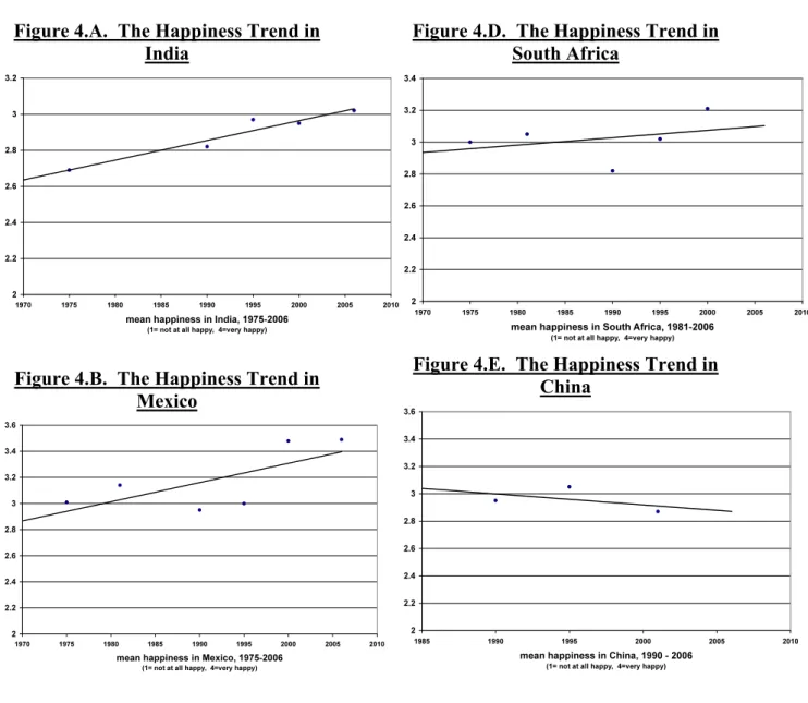
Inglehart et al. (2008) present a series of graphs plotting average happiness against time in different countries, based on the first four waves of the World Values Survey. As they point out: “in many cases, the results contradict the assumption that, despite economic growth, and

other changes, the publics of given societies have not gotten any happier. They show that the American and British series show a downward trend in happiness from 1946 to 1980, but an upward trend thereafter” [this was confirmed by Easterlin]. “In general, among the countries for which we have a long-term data, 19 out of the 26 countries show rising happiness levels. In several of these countries- India, Ireland, Mexico, Puerto Rico and South Korea- there are steeply rising trends. The other countries with rising trends are Argentina, Canada, China, Denmark, Finland, France, Italy Japan, Luxembourg, the Netherlands, Poland, South Africa, Spain and Sweden. Three countries (the U.S., Switzerland and Norway) show flat trends from the earliest to the latest survey. Only four countries (Austria, Belgium, the U.K and West Germany) show downward trends” (the Appendix to Inglehart et al., 2008). Figures 4.A to

4.E taken from their paper illustrate the positive slope of the happiness curve in India, Mexico, Puerto Rica, South Africa, and the downward slope in China.

Some work has thus uncovered a positive and statistically-significant correlation between growth and well-being over time, using within-country time-series data. This includes Hagerty and Veenhoven (2003), Stevenson and Wolfers (2008), Inglehart, et al. (2008). In turn, many of these results have been criticized by Easterlin (2005) on the basis of the choice of countries, the confusion between long-run dynamics and the business cycle, and the absence of controls in some of the estimates. Easterlin, with a number of different co-authors, has confirmed and developed his initial conjecture. Authors such as Ed Diener, Rafael Di Tella, Bruno Frey, Robert MacCulloch, Andrew Oswald and Alois Stutzer have provided additional empirical evidence in this direction.

A note on statistical power

The dispute over the long run income-happiness gradient revolves around the magnitude of the correlation coefficient and its statistical significance. A number of authors have underlined that there is less statistical power in long-run series of well-being than in the cross-section,

due to the smaller standard deviation. With less variation to explain, it is difficult to obtain statistically-significant correlations.

Hagerty and Veenhoven (2000, p. 5) for instance, note that: “the standard deviation in GDP

per capita in the cross section from Diener and Oishi was about 8000$, whereas the standard deviation in Hagerty time-series (for the same countries) was only about ¼ of that (2000$) […] within a country in 25 years”. Hence, the statistical power to detect the effect is lower in

time-series work. Equally, Kenny (2005), using data on 21 Transition and developed countries, found a standard deviation in happiness over time within countries of 0.28 on average, as compared to a standard deviation of average scores across countries of 0.65 (p. 212). Layard et al. (2010, p. 161), using Eurobarometer time series for 20 Western European countries, also report an average standard deviation of national happiness scores over time of 0.2, as compared to an average of 0.5-0.6 in the individual cross-sections.

We calculated the standard deviation in happiness and life satisfaction in the World Values Survey sections from 1981 to 2007. The average standard deviation within a cross-section (250 observations) is 0.67 for happiness (4-point scale) and 2.14 for life satisfaction (10-point scale). But the standard deviation of average national happiness across countries is 0.28 for happiness and 1.04 for life satisfaction. Finally, the standard deviation of national happiness over time fluctuates around 0.1 for happiness and from 0.13 to 0.41 for life satisfaction. In other words, the variability of subjective well-being measures is much lower in time-series than in the cross-sections within countries and across-countries. The implication is that the difference between cross-sectional versus time-series correlation coefficients is difficult to interpret.

In summary, the long-run relationship between GDP growth and subjective well-being is still a subject of some controversy. As pointed by Stevenson and Wolfers (2008), one cannot reject the null that the correlation coefficient is equal to zero, but this does not mean that one can reject the null that it is greater than zero. The nature of the long-run relationship between GDP and well-being is far from being firmly established.

I.5 Subjective well-being and the business cycle

One of the reasons why it is difficult to admit no correlation between income and well-being is that this appears in sharp contradiction to the undisputed welfare effect of the business cycle.

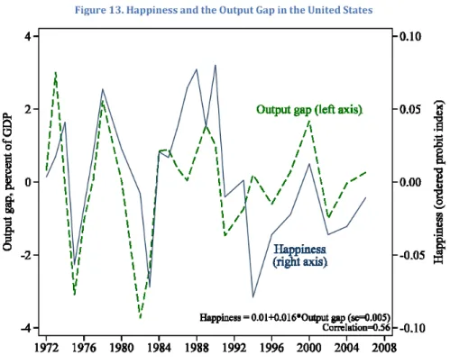
There is first of all considerable consensus that recessions make people unhappy. Di Tella et al. (2003) showed that macroeconomic movements, in particular unemployment, inflation and the volatility of output exert strong effects on the happiness of nations. The negative impact of volatility on subjective well-being was also established by Wolfers (2003). A powerful illustration of the business cycle-happiness correlation is given in Figure 5.A, taken from Stevenson and Wolfers (2008), which shows the spectacular parallel dynamics of the output gap and the average happiness in the United States from 1972 to 2008. This does not mean that the influence of the business cycle can be equated with the influence of long-run growth, however. It is indeed easy to imagine happiness and the business cycle fluctuating around a flat long-run trend. While it is uncontroversial to say that happiness rises in booms and falls in busts, the key question is whether four percent growth in GDP per annum (for example) will produce a happier society in the long run than one percent GDP growth per annum.

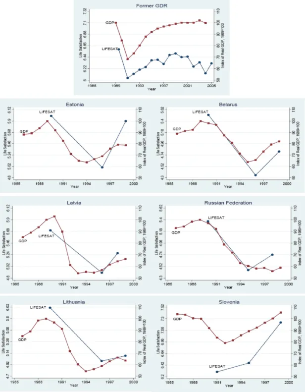
One particular episode which is often considered as an illustration of the correlation between income fluctuations and well-being, rather than between long-term growth and well-being, is the transition process in Central and Eastern European countries from socialism to capitalism. All of the work here recognizes the statistically-significant correlation between the dynamics of GDP and that of subjective well-being. Figures 5.B to 5.D, taken from Guriev and Zhuravskaya (2008) and Easterlin (2009), illustrate the concomitant evolutions in income and happiness in a number of transition countries. Similar evidence can be found in Sanfey and Teksoz (2008).

However, these trends are qualified as short term by Easterlin and Angelescu (2009), who warns that one should avoid “confusing a short-term positive happiness-income association,

due to fluctuations in macroeconomic conditions, with the long-term relationship. We suggest, speculatively, that this disparity between the short and long-term association is due to the social psychological phenomenon of “loss aversion”.

However valuable the interpretation in terms of loss-aversion, it is perhaps surprising that Transition is considered to be only a short-term phenomenon. In a way, Transition is the best example of regime change that we can think of. It is a deep and irreversible structural transformation, not a short-lived phenomenon. It shares the essential features of development, including the take-off period and the profound qualitative and institutional changes. Hence, whether Transition should be treated as a short-term or a long-term phenomenon remains an

subjective well-being continues with GDP growth, stagnates at a certain point, or falls back down to the initial (1990) level.

II. E

:

NEGATIVE SIDE

-

The flatness of happiness curves is therefore consistent with GDP growth not yielding higher well-being over time. More generally, it may suggest that whatever changes a country experiences over time have no long-run effect on individual average happiness. If this is true, the prospect is dark for developing countries, which are locked in at their current low level of happiness. The message is also very discouraging for public policy in general: if happiness cannot be raised in the long run, not only should growth be abandoned as an objective, but so should any other public policy measure.

Before jumping to these radical conclusions, the two next sections discuss possible explanations of the flatness of the happiness curve. A first series of explanations pertain to the nature of growth itself, i.e. the channels of growth and the fact that growth is accompanied by negative externalities (pollution, inequality etc.) that cancel out its subjective benefits. The second series of explanations cover social and psychological processes, such as comparisons and adaptation, that may well reduce the happiness benefits of growth.

II.1 Quality of Life: channels from GDP growth to happiness

Statistical estimates of subjective well-being most often include time and/or country fixed effects, as well as other controls that are introduced in order to pick up any changes in the demographic composition of the population (in terms of age, occupation, health, number of children, etc.). Some analyses also control for political variables such as democracy, gender equality, trust, etc. However, in terms of the empirical strategy retained for the estimation of the relationship, there is always a trade-off between controlling for variables that reflect the channels via which the phenomenon under consideration works, and not controlling for omitted variables and obtaining a biased measure of the relationship. For example, in the context of the current question of growth and well-being, a well-being regression that controlled for both GDP and the positive side-effects (or channels) of growth runs the risk of concluding that growth doesn’t matter for well-being. Indeed, we expect growth to bring about higher well-being not only via greater purchasing power (income), i.e. through higher

consumption, but also via other transformations (education, health etc.) which accompany the growth process. Controlling for these latter transformations may render GDP itself insignificant in a well-being equation, but that does not mean that greater income does not produce greater happiness, it rather means that we have identified the different processes via which income produces well-being.

Greater income per capita always comes with increased labour productivity, which means a greater choice in time-use for those who are concerned. As argued by Sen (2001), it is because it enhances the freedom of choice (by enlarging their set of capacities) that growth is expected to raise people’s well-being. Identically, GDP growth is known for being associated with demographic transitions in developing countries. This is certainly “a revolutionary

enlargement of freedom for women”, as put by Titmuss (1966, quoted by Easterlin and

Angelescu 2007, p. 9), and a rise in the education and resources for self-development that children can count on. Growth also comes with higher life expectancy, reduced child mortality and child underweight (see for instance Becker, Philipson and Soares, 2005 and Easterlin and Angelescu, 2007). Finally it is well-known that democracy and development go

hand in hand, even if the direction of causality is not as clear as was believed in the 18th

Century (e.g. by Montesquieu, Steuart and Hume). Lipset (1959, p. 80), for example, claims that: “industrialization, urbanization, high educational standards and a steady increase in the

overall wealth of society [are] basic conditions sustaining democracy”. Without inferring any

causality, we can observe the statistical association between GDP growth and progress in terms of political freedom and human rights. With respect to the empirical strategy, any attempt to capture the global effect of GDP growth on subjective well-being should not control for any such variables which represent the channels of transmission. It is likely regrettable that much of the work on the GDP growth-happiness relationship does indeed include such controls.

The following sections review the available evidence on the correlation between GDP growth and such quality of life indicators. These latter are measures of the non-income quantitative and qualitative dimensions that constitute the channels from income growth to well-being.

a. Cross-section correlation between GDP growth and Quality of Life indicators

Easterlin and Angelescu (2007) illustrate the sizeable positive correlation in cross-section data between a number of quality of life indicators and GDP per capita across countries at different

levels of development. The clear upward slopes relate subjective well-being to quantifiable factors, measured on continuous scales. These latter include food, shelter, clothing and footwear, energy intake, protein intake, fruit and vegetables, radios, cars, TV sets, mobile phone subscriptions, internet users, urban population, life expectancy at birth, gross education enrolment rate, and the total fertility rate. These kinds of relationships have been documented by a considerable number of other authors, including Inglehart and Welzel (2005), Inglehart et al. (2008), Layard et al., 2010, Di Tella and MacCulloch (2008), and Becker et al. (2005). Along analogous lines, some authors have insisted on the relationship between subjective well-being, on the one hand, and procedures, governance and institutions, democratic and human rights, tolerance of out-groups, gender equality, on the other (for example, Barro 1997, Frey and Stutzer 2000, Inglehart and Welzel 2005, Schyns 1998, and Inglehart et al. 2008).

b. Time-series correlation between GDP growth and Quality of Life indicators

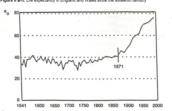
Figure 7 illustrates the spectacular take-off of life expectancy in England and Wales in the

19th century. More generally, Easterlin and Angelescu (2007) provide a detailed account of

the progress in the different dimensions of quality of life over time, in a large set of developed and emerging countries. They document the different dimensions of changes in the Quality of Life during “modern economic growth”. The latter is defined as a “rapid and sustained rise in

real output per head and attendant shifts in production technology, factor input requirements, and the resource allocation of a nation”, where “rapid and sustained” is defined as being

equal to at least 1.5% per year (Easterlin and Angelescu, 2007, p. 2).

Easterlin and Angelescu document the turning points in GDP growth and other indicators of the Quality of Life. Although both variables move in parallel, they insist that the dates of their respective take-offs do not systematically coincide. Qualitative indicators sometimes lag behind and sometimes are lead the date of GDP take-off. “If social and political indicators of

QoL are, at present, positively associated with GDP per capita, it is often because the countries that first implemented the new production technology underlying modern economic growth were also the first to introduce, often via public policy, new advances in knowledge in the social and political realms” (Easterlin and Angelescu, 2007, p. 21). Whether the

co-movements between growth and quality of life indicators represent a causal relationship is controversial and difficult to establish (see also Easterly, 1999). However, it is undeniable that overall there is no progress in quality of life without GDP growth.

In their provocative paper “Is growth obsolete?”, William Nordhaus and James Tobin (1973) advocated for an alternative indicator, integrating leisure, household work, costs of urbanization, and constructed a “Measure of Economic Welfare”. However, this index turned out to grow in a way that was similar to GDP over the period under study, albeit more slowly. This, to our knowledge is a universal observation. Pritchett and Summers (1996), for example, note that “wealthier is healthier” in the long run. Using time-series data from a variety of countries, they find that “The long-run income elasticity of infant and child mortality in

developing countries lies between 0.2 and 0.4”. This implies that “over a half a million child deaths in the developing world in 1990 alone can be attributed to the poor economic performance in the 1980s”.

In summary, GDP growth goes hand-in-hand with a series of quantitative and qualitative non-monetary improvements in quality of life. These constitute the channels from growth to well-being that we argue should not be controlled for in the statistical analysis of the former relationship.

II. 2. Negative side-effects of growth

The flatness of the GDP-happiness graphs may be due to the negative influence of some side-effects of growth, such as pollution, income inequality, work stress, and so on. The influence of these “omitted variables” could then well hide the positive influence of GDP growth on subjective well-being in econometric analyses (see Di Tella and MacCulloch, 2008).

The most widely-discussed negative side-effects of growth are: inequality, crime, corruption, extended working hours, unemployment, pollution and other environmental degradation (as measured by SOx emissions, for example). These are discussed in Di Tella and MacCulloch (2003 and 2008). Kenny (2005) also emphasises the social cost of economic transformation, and the ensuing shift from local to global relative income concerns. The impact of urban concentration and sub-urbanization is not so clear-cut, however. Easterlin and Angelescu (2007) also underline the effects of carbon dioxide emissions and fat intake (obesity and blood pressure). Clark and Fischer (2009) provide a useful summary of the macro-economic correlates of life satisfaction in OECD countries.

Among the list of usual suspects, income inequality occupies a particular place. In the first place, the relationship between income inequality and subjective well-being has been the

correlation (see Senik, 2009, for a survey, and Clark et al. 2008 and Alesina and la Ferrara, 2008, for surveys of the self-reported demand for income redistribution). Income inequality will reduce well-being if people dislike it as such (although, on the other hand, it will be associated with higher well-being if it is interpreted as reflecting a greater scope of opportunities: see Alesina et al., 2004). However, it can also exert a mechanically negative effect on average SWB, due to the concave relationship between income and SWB (see Stevenson and Wolfers, 2008). However, this mechanical effect does not seem to be sufficient to explain the flatness of the curve. As illustrated by the different panels of Figure 8 (taken from Layard et al., 2010, p. 142), income inequality increased sharply from 1970 to the end of the 2000s, but average happiness has remained flat. In addition, the income of the upper quintile of the income distribution has risen, but the happiness scores within this quintile have not. Hence, even for highest income quintile, the happiness curve has remained flat in the USA.

One important note that can be made here is that many of the negative externalities of growth seem to exhibit an inverted U-shape, i.e. they increase in the initial stages of development and then subsequently fall in the later stages. Income inequality, pollution, long hours of work, poor working conditions, etc. are phenomena that initially seem to have grown in importance with income growth, but which have then been attenuated at some point in high-income countries. This is not only the result of purely mechanical forces, but also of public policy: this is an important point to make in the context of developing countries. Should these negative factors then be taken into account when evaluating the effect of GDP growth on well-being? This an open question. If these negative side effects constitute inevitable companions to growth, then the answer is Yes: they have to be counted negatively in the welfare accounting of growth. However, if these side-effects can potentially be attenuated or suppressed by public policy, then they are not necessarily intimately linked with higher income, and as such their well-being effect can be removed from the welfare effect of growth.

III. E

(

)

III.1. Income comparisons

One simple explanation of the lack of any long-run relationship between income and well-being is that this does not reflect that there is something wrong with growth per se, but rather