HAL Id: halshs-01983037
https://halshs.archives-ouvertes.fr/halshs-01983037v4
Preprint submitted on 3 Nov 2020
HAL is a multi-disciplinary open access
archive for the deposit and dissemination of
sci-entific research documents, whether they are
pub-lished or not. The documents may come from
teaching and research institutions in France or
L’archive ouverte pluridisciplinaire HAL, est
destinée au dépôt et à la diffusion de documents
scientifiques de niveau recherche, publiés ou non,
émanant des établissements d’enseignement et de
recherche français ou étrangers, des laboratoires
Cheap talk, monitoring and collusion
David Spector
To cite this version:
WORKING PAPER N° 2019 – 03
Cheap talk, monitoring and collusion
David Spector
JEL Codes:
Keywords:
Cheap talk, monitoring and collusion
David Spector
∗October 2020
Abstract
Many collusive agreements involve the exchange of self-reported sales data between competitors, which use them to monitor compliance with a target market share allocation. Such communication may facilitate collu-sion even if it is unverifiable cheap talk and the underlying information becomes publicly available with a delay. The exchange of sales information may allow firms to implement incentive-compatible market share reallo-cation mechanisms after unexpected swings, limiting the recourse to price wars. Such communication may allow firms to earn profits that could not be earned in any collusive, symmetric pure-strategy equilibrium without communication.
1 Introduction
The objective of this paper is to better understand the role of communication in collusive practices.
Collusion, whether tacit of explicit, requires mutual monitoring.1 In many
recent cartel cases, monitoring took place by having companies compare each other’s self-reported sales with some agreed-upon quotas, with a high frequency (often, weekly or monthly). However, these sales reports were for the most part not verifiable, at least in the short run. For instance, in several cases, reliable sales information was available only with a lag of about one year.
Prima facie, this observation is puzzling. If the goal of monitoring is to deter deviations from a collusive agreement, why couldn’t a firm wanting to deviate
∗Paris School of Economics and CNRS. Email: spector@pse.ens.fr
1Sugaya and Wolitzky (2018a) show that this general statement is not as universally valid
as is often believed, because too precise information on competitors’ actions may increase a firm’s incentive to deviate from a collusive equilibrium by helping it to identify profitable deviation opportunities.
simply undercut its competitors and misreport its sales at the same time? At first glance, it seems that the only constraint on a firm’s incentive to deviate is the amount of time elapsing between the date a deviation occurs and the date it is bound to being revealed to competitors, as reliable sales data become public. How, then, could the exchange of sales reports facilitate mutual monitoring and collusion if it occurs long before sales data can be verified?
Answering this question would contribute to the ongoing debate on the an-titrust treatment of information exchanges. In the absence of direct evidence of cartel behavior, competition authorities face a difficult tradeoff. On the one hand, an outright ban on information exchanges would deny companies and con-sumers the procompetitive benefits that such exchanges may entail. Conversely, a too lenient approach would allow companies to engage in practices that could facilitate collusion and harm consumers.2
For instance, in its guidelines on horizontal co-operation between undertak-ings,3 the European Commission states that exchanges of information on past
sales are not prohibited per se (unlike communication on future behavior) and that they should be assessed under a case-by-case approach. According to K.-U. Kühn, a former Chief Economist of the European Commission, this case-by-case approach should focus on the ‘marginal impact’ of the information exchanges under scrutiny on the likelihood of collusion.4
Accordingly, this paper is an attempt to assess the marginal impact of the early disclosure of sales information long before it becomes public. When ‘hard’ information is publicly available in any case, should early disclosure be con-sidered harmless cheap talk or a practice facilitating collusion relative to a no-communication benchmark?
We construct a model showing that, in a market where demand is uncertain and sales data become available with a delay, early communication on sales volumes may make collusion more efficient. Communication may reduce the recourse to price wars as a disciplining device by ensuring that unexpected market share swings are swiftly identified and compensated through short phases of market share reallocation.
Our main finding is that, for some parameter values, collusion with
near-2See Kühn (2001).
3Official Journal of the European Union, C 11/91, 14.1.2011, Communication from the
Commission — Guidelines on the applicability of Article 101 of the Treaty on the Functioning of the European Union to horizontal co-operation agreements.
4Kühn (2011) advocates “an analysis of the marginal impact of the information exchange
on monitoring or the scope for coordination in the market. If the marginal impact appears small, the case should be closed.”
monopoly pricing in all periods along the equilibrium path can occur only if communication is possible, even though such communication does not increase data verifiability.
The collusive equilibrium we derive involves no need for contact between competitors beyond the exchange of sales reports: it is symmetric, which limits the need for pre-play coordination. It involves pure strategies along the equilib-rium path, with no need for coordination on a public randomization device. It does not involve interfirm payments.
This suggests that competition authorities should be wary of exchanges of information on past sales, even if they appear to be mere cheap talk and there is no evidence of other interfirm contacts: by itself, such communication can make collusion more efficient and lead to higher prices. Another possible interpreta-tion is that competiinterpreta-tion authorities should be wary of exchanges of verifiable information on past sales even if such exchanges take place with a long lag, because they can facilitate collusion if they are supplemented with cheap talk taking place with a shorter lag.
The main features of the collusive equilibrium derived in this paper The collusive equilibrium derived in this paper exhibits features similar to those observed in many recent cartels.5
• The collusive scheme is based on a target market share allocation. This is indeed the case in many cartels, especially in markets in which prices are not easily observed.
• Colluding firms exchange detailed information on sales volumes at a high frequency. For several cartels, the frequency of such communication was monthly (lysine,6zinc phosphate7, citric acid8), or weekly (vitamins9).
• When the exchange of self-reported sales data points to a discrepancy be-tween actual and target market shares, companies that sold above their quotas take steps to decrease their sales. According to Harrington (2006),
5Harrington (2006), Levenstein and Suslow (2006).
6Official Journal of the European Union, L 152/24, 7.6.2001, Case COMP/36.545/F3
-Amino Acids, Decision of June 7, 2000, recital 100.
7Official Journal of the European Union, L 153/1, 20.6.2003, Case COMP/E 1/37.027
-Zinc phosphate, Decision of December 11, 2001, recital 69.
8Official Journal of the European Union, L 239/18, 6.9.2002, Case COMP/E 1/36.604
-Citric acid, Decision of December 5, 2001, recital 100.
9Official Journal of the European Union, L 6/1, 10.1.2003, Case COMP/E 1/37.512
whereas in some cases cartelists compensated market share swings by mak-ing payments to each other (often under the guise of interfirm sales), in other cases the compensation was through market share reallocations of the kind highlighted in this paper, as the continuous monitoring of sales volumes afforded colluding firms “the opportunity to adjust their sales”. For instance, “the citric acid and vitamins A and E cartels engaged in ‘continuous monitoring’ to assess how sales matched up with quotas and, where a firm was at a pace to sell too much by the year’s end, the firm was expected to slow down its sales”. Likewise, in the zinc phosphate cartel, “customer allocation was used as a form of compensation in the event of a company not having achieved its allocated quota.”10
• Self-reported sales volumes are not instantaneously verifiable, but they can be compared to reliable data that become public with a lag. This information structure is in line with the facts of several cartels. Reli-able information can come from companies’ annual reports, verification by independent auditors appointed by the cartelists, import statistics, or the (delayed) publication of tender results. In several recent cases, market share information was found to become available with a delay of about one year.11 For instance, in the lysine cartel, “ADM reported
its citric acid sales every month to a trade association, and every year, Swiss accountants audited those figures.”12In the Copper Plumbing Tubes
cartel,13 import statistics were a reliable source of information on some
producers’ sales and helped cartel members to monitor the veracity of
10One feature of our collusive equilibrium does not coincide with the abovementioned
char-acteristics. The collusive equilibrium we focus on prescribes firms to adjust market shares as soon as sales reports point to a discrepancy relative to target market shares. Whereas such high-frequency adjustments indeed took place in some cases, it appears that they were not prescribed by the collusive agreement, in the sense that a firm’s failure to decrease its market share right after communication revealed that it had sold too much was not considered a deviation and did not trigger a punishment phase. This might be explained by the fact that delaying the ’rebalancing’ of market shares allows firms to average out random demand shocks and hence reduce the total amount of (often inefficient) market share reallocation.
11In our model, we make the strong assumption that the data that become publicly known
after a delay are accurate and detailed, whereas in reality they may be noisy and imprecise. Firms may try to conceal some sales from auditors, as noted by Harrington and Skrzypacz (2011); and firms’ annual reports, just like cross-country trade data, may not be very disag-gregated. However, it must also be noted that the degree of detail that is assumed in our model is not necessary for our results to hold: the assumption that total market sales become public with a lag, without the breakdown by company, would leave our results unchanged.
12Lysine decision, recital 100 (underlined by us).
13Official Journal of the European Union, L 192/21, 13.7.2006, Case COMP/E1/38.069
the previously exchanged reports,14 just like Japanese export statistics
allowed companies to check Japanese manufacturers’ sales reports in the sorbates cartel.15 In the Citric Acid cartel, companies reported
informa-tion on sales every month16and “the sales figures reported [were] audited
by the Schweizerische Treuhandgesellschaft, Coopers & Lybrand, which deliver[ed] a regular report on its findings”. 17
Overview of the mechanism at stake The possibility that firms could collude more efficiently by exchanging reports on their own sales may seem sur-prising because such reports provide no verifiable information in addition to the one that becomes public with a delay in any case. It arises from the following difference between the deterrence of undercutting and the deterrence of mis-reporting: misreporting can be spotted with certainty once sales information becomes public, whereas, if demand is uncertain enough and only sales informa-tion is available, undercutting may not be distinguishable from demand shocks. This implies that misreporting can be deterred at no cost - lies are followed by price wars, but they do not occur in equilibrium - whereas the deterrence of undercutting involves a tradeoff: if sales are an imperfect indicator of behav-ior, maximal deterrence may require price wars to happen along equilibrium paths.18
This contrast underlies our main result. Since misreporting can be detterred at little cost, firms can be induced to truthfully reveal their sales before they become observable to all. This information in turn allows firms to monitor each other more efficiently.19
14“First, SANCO manufacturers (...) reported their production and sales volume figures
often on a monthly basis to the secretariat. The figures were compiled and circulated among the SANCO club members. Second, until the beginning of the 1990s, import statistics allowed the control of sales figures, since they were a reliable source for data on production volumes, at least for countries like Belgium, where only one national producer (BCZ) existed.” (Copper Plumbing Tubes decision, recital 141).
15Harrington (2006), pp. 36-37.
16“Each of the participants reported the tonnage they had sold in each region (Europe, North
America, and the rest of the world) to the secretariat of the ECAMA President by the seventh (day) of each month. In the secretariat these sales figures were assembled and then reported back to the members by telephone, broken down by firm and by region. This made it possible to monitor the relative market shares continuously.” (Citric Acid decision, recital 100).
17Citric Acid decision, recital 37. This description does not include a mention of the
frequency of these regular reports, but it suggests that it was less than every month.
18This tension was addressed for the first time in Stigler (1964). See also Green and Porter
(1984).
19In the Citric Acid decision, it is mentioned that the information exchange allowed
collud-ing firms to ’monitor the correct implementation of [the] quotas and avoid, as far as possible, the need for compensation at the end of each year’ (recital 100). In that case, the outcome
Relation to the literature The theoretical literature on the role of com-munication in collusion comprises two main sets of contributions.
Several papers address pre-play communication in the presence of private information on costs or demand.20
Another branch of the literature addresses the role of communication as a private monitoring tool in repeated games. Compte (1998) and Kandori and Matsushima (1998) derive folk theorems, showing that infinitely patient players may achieve maximum profits if they can communicate to facilitate mutual monitoring.21
Aoyagi (2002), Harrington and Skrzypacz (2011, ’HS’ hereafter) and Chan and Zhang (2015, ’CZ’ hereafter) are closely related to this paper since they address the role of non-verifiable sales reports. They show that there may exist collusive equilibria in which companies monitor each other by exchanging sales reports, even though these reports can never be verified.22
In contrast to these papers, ours provides a comparative statics result (albeit at the price of highly specific assumptions) about the incremental impact on the feasibility of collusion of communication on past market outcomes.23 Our
assumptions depart from those in Aoyagi (2002), HS and CZ. They assume that neither price nor sales data ever become public, whereas we assume sales data to become public with a delay.24 Also, HS and CZ assume that firms
can make direct payments to each other, whereas we rule out such payments. None of these features is inherently more relevant than the others, since both types of information structures and both types of corrective mechanisms are that colluding firms attempted to avoid thanks to the frequent exchange of sales reports was a need for compensating interfirm payments (which are ruled out by assumption in our model) rather than a price war (as per the theory presented in this paper). Despite this difference, this quote illustrates one of the key ideas of this paper: the role of communication on sales volumes is to allow for frequent market share adjustements so as to avoid less desirable out-comes that might occur, absent communication, if market share swings were detected with a longer delay.
20Athey and Bagwell (2001, 2008); see also Aoyagi (2007), Harrington (2017).
21See also Obara (2009). A related paper is Rahman (2014), which describes a collusive
equilibrium involving mediated or verifiable communication between firms engaged in Cournot competition.
22In Aoyagi (2002), sales reports are imprecise, as each firm reports ’low’ or ’high’ sales
depending on whether its sales are below or above a certain threshold.
23Athey and Bagwell (2001, 2008) also derive comparative statics results on the role of
communication. But they relate to a different type of communication in a different setting, namely, pre-play coordination to take into account private information on costs.
24On the general analysis of repeated games in which information on other players’ actions
is revealed with lags, see Abreu, Milgrom and Pearce (1991). Fudenberg, Ishii and Kominers (2014) study the impact of cheap-talk communication in such games. Igami and Sugaya (2019) provide a quantitative estimate of the impact of the lag on the possibility of collusion on the basis of a stylized model of the vitamins cartel.
observed. The corrective market share reallocation mechanism highlighted in this paper, however, is probably better suited to the analysis of the cases for which information exchanges are the main legal question, as least from the viewpoint of policy relevance. This is because frequent interfirm payments may provide evidence of unlawful coordination that makes the analysis of information exchanges superfluous for the legal assessment.
To our knowledge, Awaya and Krishna (2016, ’AK’ hereafter, which is ex-tended in Awaya and Krishna, 2019a) is the only paper deriving conditions under which communication on past sales increases collusive profits relative to the ’best’ equilibrium without communication. However, our model and AK’s are relevant to different settings. AK assume that sales data remain private for-ever. Also, the nature of communication and the way it affects firms’ behavior in the collusive equilibrium are very different in their model and in ours.25
Organization of the paper We start with an example based on a model characterized by lexicographic preferences in some states of the world (Section 2). We derive a necessary condition for a pure-strategy symmetric equilibrium without communication to yield monopoly profits, and a sufficient condition for such profits to be attainable with communication. These results jointly yield a sufficient condition for communication to expand the set of attainable profit lev-els. We then consider a more general model with a less special demand function (Section 3) a derive a stronger result: for some parameter values, the maximal profits attainable without communication are bounded away from those that can be attained with communication.
2 An example
The main result of this paper relies on the following ingredients: (i) sales in-formation (at the firm level, or in aggregate form) becomes public after a lag; (ii) prices are private information; (iii) demand can be zero, which prevents a firm from inferring that a rival undercut the collusive price simply by observing its own zero sales; (iv) asymmetric demand shocks are possible, so that it is not possible to infer from asymmetric market shares that a firm undercut the
25Another related paper is Mouraviev (2014), which shows that communication can increase
collusive profits, albeit in an environment very different from ours since firms can communicate verifiable information and the only limit on communication comes from the risk of being caught colluding and having to pay a fine.
collusive price; (v) aggregate demand is stochastic, so that a firm cannot infer its market share from its own sales.
The model presented hereafter relies on an admittedly special, ad hoc de-mand function. This is the price to pay in order to obtain a tractable enough model yielding a comparative statics result on the impact of communication -rather than merely the characterization of a collusive equilibrium with commu-nication -, with an equilibrium closely resembling what has been observed in several cartels.
2.1 The model
2.1.1 Supply
There are n (n 3) identical firms producing a heterogeneous good at constant marginal cost c > 0, and facing the same rate of time preference .
2.1.2 Demand
There is a continuum of consumers. Its mass is normalized to 1.
The demand function depends on the state of the world, which is drawn from some (constant) probability distribution. The draws are independent across periods. A state of the world is characterized by two parameters: total demand (which is price-inelastic), and whether demand is ’normal’ or ’biased’ towards one firm. Total demand can take any value within an interval S = [0 , Smax),
with Smax> 0.
Consumers have unit demand with valuation V > c. Demand is either ’normal’ or ’biased’, as defined hereafter.
Demand in the ’normal’ states of the world In a normal state of the world such that total demand is Q, consumers consider all n goods as perfect substitutes. Sales are equally split among all the firms setting the lowest price if that price is lower than or equal to V .
Demand in the ’biased’ states of the world In a biased state of the world, consumers have identical lexicographic preferences that are biased towards Firm i’s product for some i. In that case, sales are evenly split among all the firms setting the lowest price (provided this price is lower than V ), unless one of these firms is Firm i, in which case all the demand goes to Firm i.
The probability distribution over demand functions The following as-sumptions about the states of the world and their probability are made through-out the paper.
Irrespective of whether demand is normal or biased, the probability distri-bution over total demand is absolutely continuous.
The demand function is symmetric across firms in the sense that (i) the distribution of total demand conditional on demand being biased is independent of the identity of the firm in favor of which demand is biased; and (ii) the probability that demand is biased in favor of any particular firm is the same for all firms.
For simplicity, and without any loss of generality, we assume that total ex-pected demand conditional on demand being biased is equal to total exex-pected demand conditional on demand being normal. Let D denote this common ex-pected value.
Demand is biased with some probability ⇡B (0 < ⇡B< 1). Conditional on
demand being biased, the distribution of total demand is given by the probability density function µB(.)over (0, S
max), with µB(Q) > 0for all Q 2 (0 , Smax).
Conditional on demand being normal, the distribution of total demand is characterized by the probability distribution µN, which has an atom in zero and
is characterized by a continuous density function µN(Q) > 0for Q 2 (0 , S max).
The overall probability that demand is zero is denoted ⇡L (these notations
imply that µN({0}) = ⇡L 1 ⇡B). MaxQ µ N(Q) µN(nQ), MaxQµ N(Q) µB(Q) and MaxQµ B(Q) µN(Q) are assumed to be finite.
2.1.3 The game
The game is repeated for infinitely many periods, starting in period 1. Each period is divided into the following stages.
Stage 1. Firms simultaneously set prices.
Stage 2. The state of the world is determined at random.
Stage 3. Each firm observes the demand addressed to it and serves it. Stage 4 (when communication is possible). Firms simultaneously make a statement on their own sales.
At the end of period t, a firm observes only its own sales, the sales made by the other firms in period t 1(if t 2) and other firms’ sales reports (in the variant with communication).
when communication is not possible, a strategy is an infinite set of functions (s1, s2, ..., st, ...), where st maps all the information known to a firm at the
beginning of period t (i.e. its own past prices and sales and other firms’ past observed sales, that is, their sales till period t 2) into the set of possible prices. When communication is possible, a strategy is an infinite set of functions (sp1, sm1 , ..., s
p
t, smt ...), where s p
t maps all the information known to a firm at the
beginning of period t (i.e. its own past prices and sales and other firms’ past observed sales and reports) into the set of possible prices, and sm
t maps all the
information known to a firm at the end of period t (i.e. the information known at the beginning of the period plus its own period t price and sales) into the set of possible sales reports.
2.2 The scope for collusion without communication
In this section, we address the scope for collusion when communication is impos-sible. We restrict our attention to pure-strategy equilibria, which is in line with our focus on simple collusive behavior.26 Also, we only consider equilibria that
are symmetric in the sense that a firm’s strategy is invariant to a permutation of other firms’ identities, and all firms follow the same strategy.27
We derive in this section a sufficient condition for the expected payoffs of pure-strategy, subgame-perfect symmetric equilibria (hereafter, ’PSSE’) to be strictly smaller than those corresponding to monopoly profits, that is, (V c)D
1 ,
when communication is not possible. We start by introducing the following notation: A = M ax ✓ µN ✓✓ Smax n , Smax ◆◆ , µB ✓✓ Smax n , Smax ◆◆◆
Proposition 1. If the inequality
1 + + 2+ (1 A) 3> 1
n (1 ) (1)
holds, then in any PSSE, the expected sum of total discounted profits is strictly
26Several recent papers, such as Acemoglu, Bimpikis and Ozdaglar (2009) and Gentzkow
and Kamenica (2017) focus on equilibria involving pure strategies along all equilibrium paths, allowing however mixed strategies off equilibrium. It must be acknowledged however that collusive behavior based on mixed strategies along the equilibrium path seems to be observed in some industries (Wang, 2009), in line with theoretical results showing that mixing can improve efficiency (Kandori and Obara, 1998).
27Models of collusion often make this assumption (see the discussion in Athey, Bagwell and
below (V c)D
1 .
Consider a hypothetical PSSE, denoted Eq⇤, that is efficient, in the sense
that the expectation of the sum of total discounted profits is (V c)D
1 in every
period. We will prove that (1) cannot hold.
Since total per-period profits cannot exceed (V c)Dand symmetry implies that the expected sum of future discounted profits is identical for all firms, the right-hand side of (1) is equal to each firm’s expected sum of future discounted profits, divided by (V c)D. We show now that each of the four terms in the left side of (1) is a lower bound on the profit (divided by (V c)D) that a firm could earn in each of the first four periods respectively by slightly undercutting its competitors, assuming these competitors set prices according to Eq⇤.
Because of symmetry, Eq⇤prescribes all firms to set the same price in period
1. Efficiency implies that this price is V .
Assume that Firm 1 deviates in period 1 and slightly undercuts its competi-tors. This affords Firm 1 an expected profit arbitrarily close to (V c)D in period 1. This corresponds to the first term in the left side of (1).
Efficiency requires the minimum price to be V with probability 1 along all possible equilibrium paths of Eq⇤(except possibly for a zero-probability subset
of such paths). Since there exists a (nonzero probability) equilibrium path such that all firms sell zero at the end of period 1 (in case demand was zero in period 1), efficiency and symmetry jointly imply that according to Eq⇤, a firm that sold
zero at the end of period 1 sets price V at the beginning of period 2. Therefore, having slightly undercut its competitors in period 1, which causes all other firms to sell zero and set again their prices at V at the beginning of period 2, Firm 1 can undercut its competitors again in period 2, which yields an expected period 2 profit arbitrarily close to (V c)D. This corresponds to the second term in the left side of (1).
At the beginning of period 3, after such deviations occured in the first two periods, Firm 1’s competitors have two additional pieces of information. Each observes that it sold zero in period 2, and that in period 1 all firms but Firm 1 sold zero and Firm 1 sold some amount D1. This information is compatible
with some equilibrium path - for instance, zero demand in periods 1 and 2 if D1 = 0, or biased demand in period 1 followed by zero demand in period 2
if D1 > 0. Because of efficiency, Eq⇤ thus requires Firms 2 to n to set prices
greater than or equal to V in period 3, except possibly for some set S1 of
values of D1 such that µB(S1) = 0, which implies µN(S1) = 0because µ
N(Q)
bounded. Therefore, with probability 1, Firm 1 can earn an expected period 3 profit arbitrarily close to (V c)D in period 3 after undercutting in periods 1, 2 and 3. This is reflected in the third term in the left side of (1).
At the beginning of period 4, Firm 1’s competitors have two new pieces of information: their own zero sales in period 3, and Firm 1’s period 2 sales. Their own period 3 zero sales provide no definitive information on Firm 1’s period 3 behavior, as zero sales could have been caused by zero demand. Consider now the information conveyed by Firm 1’s period 2 sales. For any Q 2⇥0,Smax
n , let
p⇤
2(Q) denote the price which, according to Eq⇤, a firm should set in period 2
after having sold Q in period 1 (symmetry implies that this distribution depends on Q but not on firm identity). If demand is normal in period 1 and total demand is nQ, then according to Eq⇤ each firm observes that it sold Q and sets price
p⇤
2(Q) = V in period 2 (because of efficiency and symmetry) except possibly for
a subset S2 of values of Q such that µN(nS2) = 0(with obvious notations),
which implies µN(S2) = 0because µN(Q)
µN(nQ) is bounded. Since a firm cannot observe other firms’ sales, a firm that benefitted from biased demand in period 1 and sold Q 2⇥0,Smax
n
✏
S2 also sets p⇤
2(Q) = V, leaving the possibility that
it will have a 100% market share in period 2 if it benefits from biased demand again. There exists therefore a positive-probability set of equilibrium paths such that Firm 1 has 100% market share in periods 1 and 2 with period 1 sales smaller than Smax
n . Because of efficiency, Eq⇤prescribes Firms 2 to n to set the
monopoly price in period 4 after observing such a history (and their own zero sales in period 3). Therefore, if Firm 1 slightly undercuts rivals in periods 1 to 3 and D12⇥0,Smaxn ✏S2, which happens with probability at least 1 A, then
Firms 2 to n set prices in period 4 that are greater than or equal to V , allowing Firm 1 to undercut them again - hence the fourth term in the left side of (1).
If Eq⇤is an equilibrium, the corresponding sum of discounted expected
prof-its for a firm, equal to the right side of (1) times (V c)D, should be greater than the profits induced by slightly undercutting in the first four periods, which, as is proved above, is greater than the left side of (1) times (V c)D.28 QED
28Even though the probability that a profitable deviation can occur in period 4 depends on
the realization of demand in period 1, the corresponding expected payoff is still arbitrarily close to (V c)Dbecause demand realizations are independent across periods.
2.3 The scope for collusion with communication
2.3.1 An informal overview of the role played by communication To understand the role of communication, it is helpful to go back to the mech-anism underlying Proposition 1. The reason why, absent communication, an efficient PSSE affords a firm the possibility to profitably undercut competitors during the first three periods with probability 1, and in the fourth period with probability at least 1 A, is that according to an efficient PSSE, a firm cannot be required to decrease its sales until it knows for sure that demand was biased in its favor. With probability at least 1 A, a firm observing its sales cannot know whether they represent 100% of a small demand pool or 1/n-th of a large one. A firm that was lucky in period 1 learns it in period 2, is expected to decrease its sales in period 3, and compliance with this requirement in observed at the end of period 4.
We consider now the same environment as before, with one addition: at the end of every period, each firm is required to report its sales. The key to the main result is that such communication can expose deviations sooner. To show this, we construct an efficient PSSE with communication, which has the property that a hypothetical deviator would be exposed at the end of period 3 at the latest. Consider a firm undercutting competitors in period 1 and then enjoying a 100% market share. If this firm lies about its sales, its lie is exposed at the end of period 2. If it does not lie, then, since all firms know their market shares at the end of period 1, a ’lucky’ firm can be expected to withdraw from the market in period 2 in order to offset its period 1 luck (assuming demand in period 1 was not zero). Failure to do so would be detected as soon as period 2 sales are observed by all, namely at the end of period 3 (unless period 2 demand is zero). In either case, a deviator cannot conceal its deviation for more than three periods (leaving aside the possibility of zero demand in some periods).
Communication thus allows the existence (for some parameter values) of an efficient PSSE leaving room for profitable undercutting during three periods only, as opposed to four when communication is ruled out. This implies that incentive compatibility is easier to achieve: for some parameter values, collusion at monopoly prices is an equilibrium only if communication is possible.
2.3.2 Description of the candidate equilibrium
We consider the following strategy profiles. There exist integers k and k0and a
price pw< csuch that, at the beginning of a period, the state of the game can
be any of the following (nk + k0+ 1):
• normal collusion;
• j-th period of a price war (1 j k0);
• correction at the expense of some firm i (1 i n) (the ’targeted’ firm), with r remaining correction periods (1 r k) (nk states of the game). In a nutshell, normal collusion gives way to temporary correction phases when-ever sales reports point to asymmetric sales that are compatible with equilibrium behavior (i.e., that can be explained by biased demand). During a correction phase, the firm that sold more than the others in the last normal collusion period sells zero while others set the monopoly price V , after which firms re-turn to normal collusion. Any unambiguous evidence of a deviation (like price undercutting or sales misreporting) leads to a price war. 29 30
The expected duration of a price war and the corresponding below-cost price are such that a firm’s expected discounted sum of future profits at the start of a price war is zero. Price wars do not occur in equilibrium.
Prices and messages in the candidate equilibrium Equilibrium actions at the beginning of period t depend only on the state of the game at the begin-ning of period t:
• If the state of the game at the beginning of period t is ’normal collusion’, then all firms set a price equal to V ;
• If the state of the game at the beginning of period t is ’collusion with a correction at the expense of Firm i’, then Firm i sets a price equal to V + 1 whereas all other firms set a price equal to V ;
29As is explained below, transition rules are a bit more complex than this summary
de-scription, to account for the possibility that during a correction phase at the expense of some firm, another firm may benefit from biased demand and become the target of a new correction phase.
30That price wars cannot occur in equilibrium is in constrast to HS. In HS, the incentive
not to misreport sales results from the existence of a function associating to each vector of sales reports the probability of a shift to a noncollusive phase. This function is such that truth-telling is an equilibrium. In our model, the assumption that sales data become public with a lag allows for a simpler mechanism: lies trigger price wars once they are detected.
• If the state of the game at the beginning of period t is ’price war’, then all firms set a price equal to pw.
Also, in the candidate equilibrium, firms truthfully report their sales.
Transitions between states of the game in the candidate equilibrium The state of the game at the beginning of period 1 is ’normal collusion’. At the beginning of period t (t 2), the state of the game is determined as follows.
• Deviations trigger a price war: if the reported period (t 1) sales are incompatible with the prices prescribed by the candidate equilibrium in period (t 1), or (if t 3)the reports on period (t 2) sales at the end of period (t 2) do not match the actual period (t 2) sales as observed at the end of period (t 1), then the state of the world in the next period is the first period of a price war.
In all other cases, that is, if the newly available information provides no evidence of a deviation, transition rules are as follows.
• Normal collusion is followed by normal collusion if period (t 1) reported sales are equal; and otherwise a correction phase with k remaining periods at the expense of the only firm that reported nonzero sales.
• Price wars start over unless reported sales are equal and strictly positive. If the state of the game at the beginning of period (t 1 )is ’r-th period of a price war’ with r k0, then (i) if reported period (t 1) sales are
equal and strictly positive, then the state of the game at the beginning of period t is ’(r +1)-th period of a price war’ if r < k0and ’normal collusion’
if r = k0; (ii) otherwise, it is ’first period of a price war’.
• At the end of a correction period at the expense of Firm i with r remaining periods, if the reported period (t 1)sales of all firms other than Firm i are equal, then at the beginning of period t the state of the game is ’normal collusion’ if r = 1 and ’correction at the expense of Firm i with (r 1)remaining periods’ if r > 1. If only one firm (say Firm j, j 6= i) reported nonzero sales, then at the beginning of period t the state of the world is ’correction at the expense of Firm j, with k correction periods remaining’.
This candidate equilibrium is symmetric, involves only pure strategies and yields expected total profits (V c)Din every period.
2.3.3 A sufficient condition for the candidate equilibrium to be an actual equilibrium
Proposition 2. If ⇡B and ⇡L are close enough to zero and there exists an
integer k such that Conditions (2) and (3)
n(1 ) (1 + ) < k (2) n(1 ) + k+1< 1 (3)
hold, then there exist a positive integer k0 and a price pw such that the above
strategy profiles correspond to a PSSE (with correction phases lasting k periods and price wars lasting k’ periods with price pw). In this equilibrium, expected
total profits are (V c)D in all periods.
Proposition 2 is a limit case of a stronger result holding under more general assumptions (Proposition 5, in the next section, the detailed proof of which is in the appendix). We provide here a sketch of the proof.
First, given the transition rules stated above and the fact that expected profits are strictly positive at the end of a price war, one can find (by continuity) a pair (pw, k0) such that, in expectation, the losses incurred during a price
war exactly offset these future profits so that a firm’s expected sum of future discounted profits at the start of a price war is zero. We consider such a pair.
Second, if ⇡B and ⇡L are close enough to zero, then undercutting leads a
deviator to have a 100% market share with a probability close to 1.
(2) can be written (1 + ) (V c)D < 1k (V nc)D . (2) implies that it is optimal for a firm targeted by a correction period to follow the prescriptions of the candidate equilibrium. If it undercuts the other firms, it earns (V c)Din expectation but its (almost certain) 100% market share willl be detected at the end of the next period, triggering a price war, so that the best it can do is report zero sales and undercut again, after which a price war starts. The deviator’s profits would thus be monopoly profits during two periods, and in expectation zero thereafter. This is captured by the left side of (2).
The right side corresponds to the expected profit of a firm complying with the prescriptions of the candidate equilibrium at the start of a correction period targeting it (namely, zero for k periods and 1/n-th of total profits thereafter): if ⇡Bis small, the correction phase will not be interrupted by the start of a new one
targeting another ’lucky’ firm. (2) implies that complying by the prescriptions of a correction period is optimal. If ⇡Band ⇡Lare close to zero, (2) also implies
that a firm that benefitted from biased demand during a ’normal collusion’ phase is better off by not lying: misreporting and undercutting would lead to monopoly profits during one additional period, which is less than the left side of (2), whereas exposing itself to a correction phase as prescribed would yield in expectation the right side.
(3) is equivalent to (V c)D + 1k+1 (V c)D n < 1 1 (V c)D n . This inequality
implies that it is optimal not to undercut in a ’normal collusion’ period: the right side is equal to the expected sum of future discounted profits of a firm complying with the prescriptions of the candidate equilibrium, whereas the left side corresponds to a specific deviation, namely undercutting and then truthfully reporting sales (which is more profitable than lying) and complying with the prescriptions of the candidate equilibrium forever after. (2) and (3) together imply that there is no profitable deviation (for a systematic analysis, see the proof of Proposition 5 in the appendix).
2.4 Comparative statics: the marginal impact of communication
Combining Propositions 1 and 2 provides a sufficient condition for communica-tion to expand the set of the profits attainable in a PSSE: this is the case if conditions (1), (2) and (3) are simultaneously satisfied.
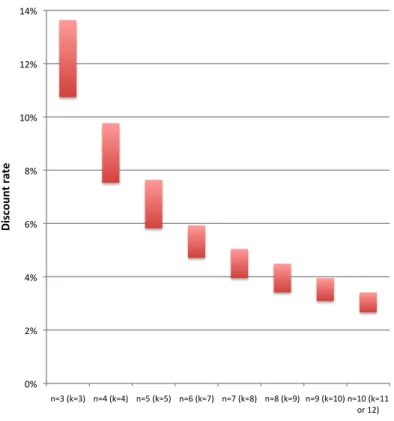
Proposition 3. For each n between 3 and 10, there exist parameter values such that, if communication is possible, there exists a PSSE leading to a discounted sum of total expected profits equal to (V c)D
1 , whereas if communication is not
possible, there exists no such PSSE.
The proof of this result (a consequence of Proposition 6, the proof of which is in the appendix) has two main parts. First, we prove that there exist triplets (n, , k)such that conditions (1)-(3) jointly hold when A = 0 (Figure 1) and, by continuity, for some strictly positive A > 0. Figure 1 displays intervals of values of satisfying (1)-(3) for selected values of n and k and A = 0 (and therefore for some A > 0 by continuity).31 Second, considering a set of triplets (n, , k)
such that (1)-(3) hold for some A > 0, we show that one can construct a family of demand functions such that ⇡B and ⇡L are arbitrarily close enough to zero
and MaxQ µ N(Q) µN(nQ), MaxQµ N(Q) µB(Q) and MaxQµ B(Q) µN(Q) are bounded. INSERT FIGURE 1.
31For the sake of readability, we present these results in terms of the discount rate applied
over a period, that is, the rate ⇢ such that = 1 1 +⇢.
2.5 The limits of the above results
The granularity of sales data. The above results do not require an infor-mational assumption as strong as ours. The strategies in the equilibrium with communication could be implemented under the weaker assumption that reli-able data on total rather than individual market sales become availreli-able after a one-period lag. Such information would allow firms to detect that some firm lied, by comparing actual and reported total sales, and comparing total reported sales with its own individual sales would allow each firm to calculate its market share. Since, in the equilibrium with communication displayed above, the price war following a lie treats all firms symmetrically, the lack of information on a liar’s identity would make no difference. Therefore, communication through a third party that collects firms’ own-sales reports and communicates to all firms total sales data based on these reports would be sufficient for Proposition 2 to hold.32
At least three firms. With more than three firms, if a firm sets a price above consumers’ valuation V in a ’normal collusion’ period, the ensuing sales distribution is incompatible with any equilibrium path if demand is neither zero nor biased since all firms but one sell nonzero amounts, and there is no way for a firm to conceal such a deviation (it could not report the same sales as other firms because it would not know them), so that a price war would ensue. With only two firms, such a deviation cannot be ruled out as simply: if a firm sets a price above the monopoly level, this would lead to sales looking like the result of biased demand in favor of its competitor, which could trigger a correction phase at the expense of this competitor. Having more than three firms dispenses us from considering such deviations.
No interfirm payments. Our results would not hold if interfirm payments were possible. In that case, a sales imbalance in period 1 could trigger
compen-32This remark is at odds with the oft-made claim that “aggregating the data [on firms’
historical and current prices, costs, and output] largely removes the value of information in facilitating collusion” (Carlton, Gertner and Rosenfield, 1997). Awaya and Krishna (2020) present another mechanism through which the communication of credible aggregate sales data to individual firms can facilitate collusion. In their model (unlike those in their 2016 and 2019a papers) firms have an incentive to misreport sales, hence the need for “Swiss accountants”. It must be noted that in some models, more accurate information may decrease the set of attainable profits because it may help firms to identify more profitable deviations (Sugaya and Wolitzky, 2018a). However, such a mechanism cannot be present in our model, since the deviations considered here do not rely on the deviating firm’s information on other firms’ sales.
sating payments at the end of period 2, just after it is publicly observed, even without communication.
Symmetric strategies. The restriction to symmetric strategies is crucial to our results. Absent this restriction, one could envision collusive equilibria with-out communication such that companies take turns and in each period, one serves the entire demand while the others set prohibitively high prices. The informational problem that communication is meant to solve would not exist because deviations would be spotted as soon as sales data become observable. Pure strategies. If mixed strategies were considered, one could envision can-didate equilibria such that prices are drawn from an atomless distribution. A firm making nonzero sales would know that its market share is 100% right af-ter observing its own sales. This would remove the informational problem that communication is meant to solve even without communication.
Lexicographic demand. This restriction, made for expositional simplicity, makes the results weaker than they would be under a less extreme modeling of demand (see below). This assumption is relaxed in the next section.
Which bound on collusive profits without communication? Proposi-tion 3 provides no lower bound on the incremental impact of communicaProposi-tion on collusive profits. In fact, under lexicographic preferences, the reasoning behind Proposition 1 cannot be extended to provide a strictly positive lower bound. A crucial step in the proof of Proposition 1 is that in an efficient PSSE without communication, a reallocation of markets shares (by having a lucky firm with-draw from the market) cannot immediately follow a market share imbalance. Reallocation can take place only after firms learn their market shares and the lucky firm realizes it was lucky. But the reason for this is the efficiency re-quirement: if the minimum price must be the monopoly price V , then a firm can withdraw only by setting a price above consumers’ willingness to pay, and it would be inefficient for all firms to do so, each wrongly believing it is the only ’lucky’ firm. However, giving up an arbitrarily small fraction of expected equilibrium profits would allow a market share reallocation phase to take place immediately after a biased demand period, without waiting for firms to learn that there was an imbalance. Consider any arbitrarily small " > 0. A strategy prescribing that a firm sets price V "after it sold zero and V otherwise would
cause a market share reallocation following biased demand, at a cost to total profits of only ". This is because under lexicographic preferences, a firm setting a price slightly above its competitors’, however small the difference, sells zero even if demand is biased in its favor. Therefore, the above results prove that communication may be required to achieve monopoly profits, but they do not prove that communication can increase the maximum attainable profits. In the next section, we prove that the above results can be strengthened under a less extreme modeling of demand: communication may increase the maximum attainable profits.
3 A more general model: communication may
in-crease the maximum attainable profits
In this section, we relax the assumption of lexicographic preferences in the case of biased demand. This allows us to state a stronger result.
3.1 Assumptions: a less special demand function
The only change in assumptions is that when demand is biased in favor of some firm, say Firm i, the relative preference for that firm’s product is stronger than implied by lexicographic demand: in that case, consumers’ valuation for product iis some v > V . It is assumed, like in the previous section, that if consumers are indifferent between the several firms’ offers, demand is split equally between them.
Consumers’ willingness to pay for product i when demand is biased in favor of Firm i is drawn from some probability distribution ⌫ over some interval (V, V0)
with V0 > V. For the sake of tractability, ⌫ is assumed to be the uniform
distribution. The ratio (V0 V )/(V c)is denoted u.
3.2 Collusion without communication
With this modified demand, Proposition 1 can be strengthened: Proposition 4 states a condition for the non-existence of equilibria approaching total expected profits of (V c)D per period, when firms cannot communicate. Its proof (appendix) is more complex than that of Proposition 1 but it follows the same logic.
Proposition 4. If inequality (1) stated in Proposition 1 holds and ⇡L, ⇡B, ⇡Bu
⇡L and
nu
(1 )3⇡B⇡L(1 A) are close enough to zero, then total expected
per-period profits in all PSSE are bounded away from (V c)D: there exists > 0 such that in any PSSE, the expected sum of all firms’ future discounted profits is smaller than or equal to (V c)D
1 (1 ).
We explain hereafter why the various expressions mentioned in the statement of Proposition 4 must be close to zero. Just like for Proposition 1, the proof is based on showing that, if a hypothetical equilibrium exists that yields total profits close enough to (V c)D
1 , then it prescribes strategies that would allow
a firm (say, Firm 1) to profitably undercut and earn in expectation almost (V c)Din each of the first four periods. Since in periods of biased demand, consumers’ willingness to pay for their favorite good is V0 > V, the greatest
possible expected total per-period profit is not (V c)D anymore but rather (V c)D(1 + ⇡Bu). ⇡Bushould be small enough so that for the sum of total
expected profits to be close to (V c)D
1 , profits must be close enough to (V c)D
in each of the first four periods (those considered in the proof). Also, a key element of the proof of Proposition 1 is that the ’suspicious’ observation that Firm 1 was the only firm with nonzero sales in periods 1 and 2, and other firms again had zero sales in period 3 is still compatible with some equilibrium path (if Firm 1’s period 1 sales were below Smax
n , so that it could not infer
it had a 100% market share) - and thus does not trigger a price war. If the question is now about approaching per period profits of (V c)D, it must be the case that the probability for this observation to occur in equilibrium (i.e., the probability of an ’innocent’ explanation for this suspicious observation) is large enough: otherwise, it could trigger a price war without much impact on total expected profits. The probability that demand is biased in the first two periods, towards the same firm, that it is zero in period 3, and that the ’lucky’ firm’s period 1 sales are below Smax
n , is greater than
(⇡B)2
⇡L(1 A)
n . This probability
should be high relative to the maximum possible ’upward’ deviation of profits in excess of (V c)D, namely ⇡Bu, which could occur in the first period and be
’compensated’ downwards during the fouth (and last) deviation period, hence the division by 3, leading to the condition that nu
(1 )3⇡B⇡L(1 A) should be
close to zero. By the same reasoning, the probability that all firms observe zero sales at the end of Period 1 is ⇡L, implying that ⇡Bu
⇡L should be close to zero. Also, since the proof is based on showing that repeated undercutting is profitable, it is facilitated by having ⇡B close to zero, since a very small price
undercutting is profitable only if demand is not biased, i.e., with probability 1 ⇡B.33
3.3 Collusion with communication
The equilibrium with communication described in Section 2 is also an equilib-rium in the modified model considered in this section, with a more general, non-lexicographic demand structure, under the same conditions on parameters, provided preferences when demand is ’biased’ are close to lexicographic. The only difference with the equilibrium strategies described in Section 2.3 is that in a correction period at the expense of a firm, that firm sets a price equal to V0+ 1, rather than V + 1 (in order to ensure zero sales).
Proposition 5. If ⇡B, ⇡L and u are close enough to zero and there exists an
integer k such that inequalities (2) and (3) stated in Proposition 2 hold, then there exist a positive integer k0 and a price pw such that the strategy profiles
described in Section 2.3 correspond to a PSSE (with correction phases lasting k periods and price wars lasting k’ periods with price pw). In this equilibrium,
expected total profits are (V c)D in all periods.
3.4 Comparative statics: the marginal impact of
commu-nication
The same comparative statics result holds as in Section 2: for some parame-ter values, communication allows firms to attain collusive profits that are not attainable without communication.
Proposition 6. For each n between 3 and 10, there exist parameter values such that, if communication is possible, there exists a PSSE leading to a discounted sum of total expected profits (V c)D
1 , whereas if communication is not possible,
this sum, considered over all PSSE, is bounded away from (V c)D
1 .
The proof of this result is in the appendix. It has two main parts. First, we prove that there exist triplets (n, , k) such that conditions (1)-(3) jointly hold when A = 0 (Figure 1) and, by continuity, for some strictly positive A > 0.
33The condition that ⇡Lshould be close to zero is not strictly necessary for Proposition 4 to
hold, but it simplifies the proof. Since the main result of the paper is Proposition 6, namely, the existence of parameters such that communication increases maximal attainable collusive profits, and the existence of a high-profit equilibrium with communication requires ⇡Lto be
small (Proposition 5, see also the informal discussion of Proposition 2), this condition does not restrict the main contribution of this paper.
Second, considering a set of triplets (n, , k) such that (1)-(3) hold for some A > 0, we show that one can construct a family of demand functions such that ⇡L,
⇡B, ⇡Bu
⇡L and (1 ) 3⇡nuB⇡L(1 A) and (1 max)3nu
min⇡B⇡L(1 A) are arbitrarily close enough to zero and MaxQ µ
N(Q) µN(nQ), MaxQµ N(Q) µB(Q) and MaxQµ B(Q) µN(Q)are bounded.
4 Conclusion
The model presented in this paper casts light on the marginal impact of commu-nication on the feasibility of collusion: the exchange of sales reports may lead to higher prices because it facilitates the recourse of colluding firms to incentive-compatible market share reallocation mechanisms, limiting the need for price wars. This result, which is similar to Awaya and Krishna’s (2016, 2019) but applies to a different information structure and involves a different relationship between the information that is exchanged and firms’ subsequent actions, may be present even though the information exchange is mere cheap talk, in the sense that it does not make sales data verifiable sooner.
While the assumption that sales data become public after a delay is strong, it nevertheless is relevant to many markets. Also, our results are robust to weak-ening this assumption. Assume for instance that sales data become public after being audited by third parties (as was the case in several cartels mentioned in the introduction as a motivation for this paper). If a firm that undercuts its competitors and increases its sales as a result can, with a small probabil-ity, succeed in concealing some sales from its auditor, then our results should carry over, since the profitability of undercutting is a continuous function of the probabilities of the various states of the world in the subsequent periods.
Turning to the implications for antitrust enforcement, our results suggest that the exchange of sales reports should be considered suspicious if reports revealing market share swings lead to prompt compensating movements, to an extent that cannot be explained by individual firms’ unilateral profit maximiza-tion behavior, given the intertemporal pattern of demand shocks. Competimaximiza-tion authorities should not rule out the possibility that communication is meant to facilitate such compensation mechanisms, even if the data that are exchanged between firms are not verifiable when communication takes place, and communi-cation does not affect the date at which they will become verifiable. Conversely, the public dissemination of verifiable sales data may conducive to collusion even if it takes place with a long lag, because it can be supplemented with private
communication on non-verifiable sales data that takes place with a shorter lag. It may therefore warrant more public scrutiny.
Also, since our results continue to hold under the assumption that the data becoming public after a lag are about total sales only, they imply that the dissemination of aggregated sales data by trade associations, based on firms’ self-reported sales, may facilitate collusion.
Admittedly, our model relies on special and restrictive assumptions about demand. This is in our view the price to pay in order to estimate an upper bound on firms’ profits in all (pure strategy, symmetric) equilibria without communication, which then allows us to state results on the marginal effect of communication. This is because little is known yet on bounds on equilibrium payoffs in infinitely repeated games under general assumptions (except at the limit when players are almost infinitely patient). However, recent advances on this topic may pave the way for additional results on the marginal impact of communication under less special assumptions.34 This should be the focus of
future research.
Appendix
Proof of Proposition 4. We introduce the following notations: 1 denotes
M ax ✓ M ax Q2(0,Smax) µN(Q) µB(Q), M ax Q2(0,Smax) µB(Q) µN(Q) ◆ and 2 denotes M ax Q2(0,Smaxn ) µN(Q) µN(nQ). We consider a hypothetical PSSE Eq⇤ such that the the expected sum of all firms’ future discounted profits is greater than (V c)D
1 (1 )for some small
. The core of this proof is the calculation of a lower bound on the profits that some firms, say Firm 1, could earn by following a certain strategy, which can be interpreted as undercutting in each of the first four periods. This requires intermediate results about the strategies followed by Firms 2 to n conditional on the information available to them.
Step 1. Minimum combined profits after certain histories. We define the his-tory of the game till period t as the sequence of prices and sales till period t in-cluded. We provide hereafter a lower bound on the expectation of total period t profits conditional on past history belonging to some set H. Let P rob(H) denote the probability, according to Eq⇤, that the history of the game till period (t 1)
34See in particular Pai, Roth and Ullman (2016) and Sugaya and Wolitzky (2017, 2018b).
Awaya and Krishna (2016, 2019a) also overcome this difficulty by characterizing an upper bound on collusive profits in the no-communication case under quite general assumptions.
belongs to H (and let it be equal to 1 if t = 1). Since total expected profits in any period cannot exceed (V c)D(1 + ⇡Bu), the expected discounted sum of total
profits in all periods cannot exceed (V c)D(1 + ⇡Bu)⇣ 1 1
t 1P rob(H)⌘+ t 1P rob(H)Q(H), whereQ(H)denotes expected total period t profits
condi-tional on past history belonging to H. This expected discounted sum is greater than (V c)D(1 ) 1 , implying that Q (H) > (V c)D(1 ↵t(P rob(H), ))with ↵t(x, ) = +⇡ Bu x(1 ) t 1.
Step 2. A quasi-lower bound on equilibrium prices. Assume that in period i, conditional on a certain event (a set of past histories), the expectation (according to Eq⇤) of total profitsQ is greater than (V c)D(1 ↵) for some ↵. Defining g(↵) = q↵+⇡Bu
1 ⇡B , the probability (conditional on that same event) that the lowest of all n prices in period i is greater than c+(V c)(1 g(↵)) is greater than 1 g(↵). Proof: total expected profits cannot exceed D Min p1
t, ..., pnt, V c
if demand is normal and (V c)D(1 + u) otherwise. If the probability that M in p1
t, ..., pnt c < (V c) (1 g(↵))is greater than g(↵), then Q (V c)D <
⇡B(1 + u) + (1 ⇡B) (1 g(↵) + g(↵)(1 g(↵))) = 1 ↵.
Step 3. The profit from deviating in period 1. Since Eq⇤ is symmetric, it prescribes all firms to set the same price p⇤
1in period 1. The total expected profit
induced by Eq⇤ in period 1 is thus less than or equal to D (p⇤
1 c) ,implying
that p⇤
1 c > (V c) (1 g1), with g1= ↵1(1, ). If Firm 1 deviates and sets a
price equal to pdev
1 = c + (V c) (1 g1)in period 1, it serves the entire demand
if demand is normal or biased in its favor, i.e., with a probability exceeding 1 ⇡B.
Step 4. Firm 1’s possible deviation in period 2. Since Eq⇤ is symmetric, there exists p⇤
2(0) such that Eq⇤ prescribes a firm that sold zero in period 1
to set price p⇤
2(0) in period 2. The equilibrium probability that all firms sell
zero in period 1 is ⇡L. Step 1 implies that p⇤
2(0) > c + (V c) 1 ↵2(⇡L, ) .
Let g2 denote ↵2(⇡L, ). If Firm 1 deviates in period 2 by setting a price
pdev
2 = c + (V c) (1 g2)and all other firms made zero profits in period 1, its
expected period 2 profit is greater than (V c)D (1 g2) 1 ⇡B .
Step 5. Firm 1’s possible deviation in period 3. For each Q in (0, Smax],
let p⇤
3(Q) denote the price prescribed by Eq⇤ in period 3 for a firm having
observed that (i) it sold zero in period 2; and (ii) in period 1, one of the firms (not itself) sold Q while all others sold 0. We also define g⇤
3(Q)by the identity
p⇤
3(Q) c = (V c) (1 g⇤3(Q)).The equilibrium probability that (i) Firms 2
to n had zero sales in periods 1 and 2 and (ii) Firm 1 had nonzero sales in period 1 is greater than ⇡B
and (ii), with probability greater than 1 g⇣↵3(⇡
B
n⇡
L, )⌘, the minimum of
all prices in period 3 is above c + (V c)⇣1 g⇣↵3(⇡
B
n⇡
L, )⌘⌘: there exists
S3 ⇢ (0, Smax) such that (i) µB(S3) > 1 g
⇣ ↵3(⇡ B n⇡L, ) ⌘ and (ii) 8Q 2 S3, g⇤3(Q) < g3.Also, by the definition of 1, µN(S3) > 1 1g
⇣ ↵3(⇡ B n ⇡ L, )⌘. Define pdev 3 = c + (V c) (1 g3) with g3 = g ⇣ ↵3(⇡ B n⇡ L, )⌘. Conditional
on Firms 2 to n having sold zero in periods 1 and 2 and on Firm 1 having made nonzero sales in period 1 (which happens with probability greater than 1 ⇡B 1 ⇡B ⇡L if Firm 1 deviated in the first two periods), if Firm
1 sets price pdev
3 in period 3, this price is lower than all other firms’ prices
with probability greater than 1 1g3, yielding an expected profit greater than
(V c) (1 g3) (1 1g3) 1 ⇡B .
Step 6. The period 2 prices set by a firm observing its period 1 sales belonged to 0,Smax
n , according to Eq⇤.
For each Q 2 0,Smax
n let p⇤2(Q)denote the equilibrium price set in period
2 by a firm observing that it sold Q in period 1. uch that a firm having sold Q in period 1. We define the set S0as follows: S0= Q s.t. Q2 0,Smax
n and p⇤2(Q) > V .
With probability 1 ⇡B µN(nS0) (with nS0denoting the set of all elements
of S0 multiplied by n), demand is normal and each firm sells some Q 2 S0 in
period 1, implying that all firms set a price strictly above V in period 2, leading to expected period 2 profits smaller than or equal to ⇡B(V c)D(1 + u). Step 1
implies therefore that 1 ↵2 1 ⇡B µN(nS0), < ⇡B(V c)D(1+u), or,
af-ter rearranging af-terms, µN(nS0) < +⇡Bu
(1 ⇡B)(1 ⇡B(1+u)) , which implies µN(S0) <
2 +⇡
Bu
(1 ⇡B)(1 ⇡B(1+u)) .
Step 7. The probability, according to Eq⇤, that Firm 1’s sales belong to 0,Smax
n \ S0 in period 1 and to (0, Smax) in period 2 while all other firms
sell zero in periods 1 and 2. According to Eq⇤, the probability that Firm 1’s period 1 sales belong to 0,Smax
n \ S0 whereas all other firms’ period 1
sales are zero is ⇡B
n 1 µ
B(S0) µB Smax
n , Smax . If Firm 1’s period 1 sales
belong to 0,Smax
n \ S0 whereas all other firms’ period 1 sales are zero, then
according to Eq⇤, in period 2 Firm 1 sets a price p⇤
2(Q) V and all other
firms set a price p⇤
2(0) > (V c) (1 g2) + c (by Step 4), so that p⇤2(Q)
p⇤
2(0) < (V c)g2, implying that the entirety of period 2 demand goes to Firm
1 if demand is biased in Firm 1’s favor and consumers’ valuation v of Firm 1’s product is such that v c
V c 1 > g2, which is the case with probability ⇡B n⌫ (((V c)(1 + g2) + c, V0)) = ⇡B n 1 g2 u if g2< u, or +⇡Bu ⇡L(1 ) < u. From
here onwards, we assume that ⇡B
⇡L is small and we consider values of that are small relative to u, so that g2< u. The probability according to Eq⇤ that firms
other than Firm 1 sell zero in the first and the second period whereas Firm 1’s sales in these periods belong respectively to 0,Smax
n \ S0 and (0, Smax)is
thus greater than ⇣⇡B
n ⌘2 1 µB(S0) µB Smax n , Smax 1 g2 u . µ B(S0) < 1µN(S0)so that (using the results of Step 6) the latter expression is greater
than⇣⇡B n ⌘2⇣ 1 1 2 +⇡ Bu (1 ⇡B)(1 ⇡B(1+u)) A ⌘ 1 g2 u .
Step 8. The period 4 prices set by all other firms after having sold zero in periods 1 to 3 and observing that Firm 1’s sales belong to 0,Smax
n \ S0 in
period 1 and (0, Smax) in period 2. The probability, according to Eq⇤, that
Firms 2 to n sell zero in periods 1, 2 and 3, while Firm 1 makes nonzero sales in periods 1 and 2, and its period 1 sales belong to 0,Smax
n \ S0, is greater than
the latter lower bound times ⇡L. Define
g4= g ↵4 ⇡L ✓ ⇡B n ◆2✓ 1 1 2 + ⇡ Bu (1 ⇡B) (1 ⇡B(1 + u)) A ◆ ⇣ 1 g2 u ⌘ , !! . Step 2 implies that conditional on Firm 1 having nonzero sales in periods 1 and 2 (belonging to 0,Smax
n \S0in period 1) and other firms having zero sales in
peri-ods 1 to 3, then with probability greater than 1 g4,Firms 2 to n set a price that
is greater than pdev
4 = c + (V c) (1 g4). Notice that the probability that after
Firm 1 deviated by setting prices pdev
i in period i (i = 1, 2, 3), its sales belonged
to 0,Smax
n \S0in period 1 and (0, Smax)in period 2 while other firms sold zero
in periods 1 to 3 is greater than⇣1 µN(S0) µN Smax
n , Smax ⇡L
1 ⇡B ⌘
1 ⇡B 3,
which is greater than⇣1 2 +⇡
Bu (1 ⇡B)(1 ⇡B(1+u)) A ⇡L 1 ⇡B ⌘ 1 ⇡B 3.
Step 9. Firm 1’s possible deviations in periods 1 to 4 and the corresponding expected profits. Steps 1 to 8 imply that if Firm 1 sets price pdev
i in period i (i =
1, 2, 3, 4)then its expected profit is at least (V c)D (1 g1) 1 ⇡B in period
1, (V c) D (1 g2) 1 ⇡B 2in period 2, (V c) D (1 1g3) (1 g3) 1 ⇡B ⇡L 1 ⇡B 2 in period 3 and (V c) D⇣1 2 +⇡ Bu (1 ⇡B)(1 ⇡B(1+u)) A ⇡ L 1 ⇡B ⌘ 1 ⇡B 4(1 g 4)2 in period 4.
Step 10. (1) implies the existence of a profitable deviation. Assume that inequality (1) holds: 1 + + 2+ (1 A) 3 > 1
n(1 ) . (1) is equivalent to 4+ A 3< 1 1
n, which provides a strictly positive lower bound on the possible
values of 1
1 . If ⇡L, ⇡B, ⇡Bu
⇡L ,
nu
(1 ) 3⇡B⇡L(1 A) and are close to zero, then