Numerical results for generalized attachment models for the genesis of graphs

(1)

HAL Id: inria-00349461

https://hal.inria.fr/inria-00349461

Submitted on 31 Dec 2008

HAL is a multi-disciplinary open access

archive for the deposit and dissemination of

sci-entific research documents, whether they are

pub-lished or not. The documents may come from

teaching and research institutions in France or

L’archive ouverte pluridisciplinaire HAL, est

destinée au dépôt et à la diffusion de documents

scientifiques de niveau recherche, publiés ou non,

émanant des établissements d’enseignement et de

recherche français ou étrangers, des laboratoires

the genesis of graphs

Jens Gustedt, Pedro Schimit

To cite this version:

Jens Gustedt, Pedro Schimit. Numerical results for generalized attachment models for the genesis of

graphs. [Technical Report] RT-0361, INRIA. 2008, 74 p. �inria-00349461�

(2)

a p p o r t

t e c h n i q u e

ISRN INRIA/R T --0361--FR+ENG Thème NUM

Numerical results for generalized attachment models

for the genesis of graphs

Jens Gustedt — Pedro Schimit

N° 0361

(3)

(4)

Centre de recherche INRIA Nancy – Grand Est

models for the genesis of graphs

Jens Gustedt, Pedro Schimit

Thème NUM — Systèmes numériques ´

Equipe-Projet AlGorille

Rapport technique n➦ 0361 — December 2008 — 71 pages

Abstract: Using the network generation model from Gustedt [2008], we simu-late and analyze the clustering coefficient of the networks as some parameters changes

(5)

mod`

eles d’attachement pour la g´

en`

ese de

graphes

Résumé : En utilisant le modèle de génération de réseaux de Gustedt [2008], nous simulons et analysons le coëfficient de clustering de ces réseaux en variant certains de leurs paramètres

(6)

1 Introduction and Overview

A model proposed in Gustedt [2008] is used for the random generation of large sparse graphs that allows to produce families of graphs with non-vanishing clus-tering coefficient. The main objective of this paper is to observe the depen-dency of the clustering coefficient as some parameters to generate the graphs are changed.

In Section 2, we present the model, some of its variations, and relate it to some well-known random models of networks (e.g. Barab´asi and Albert [1999], Erd˝os and R´enyi [1960]). We compare the models and presentation of the different simulation that were realized and the justify our choices for the genesis of the graphs and related computations, in particular the computation of the clustering coefficient.

In Section 3, all the results of our simulations are presented, analyzed and discussed. Furthermore, a graphical view is used to have another idea of what happens with the graph for the different used parameters. In Section 4, our conclusions are presented.

All figures are given in the Appendix, see page 15 for a table of contents.

2 Model

The model of reference for our genesis of generation of graphs can be described basically with two types of entities: contexts and objects which are considered a level up of organization for nodes and edges in a graph.

In our graph a observer is a node and a group of observers compounds a context. If a context co have the objects ob1, ob2 and ob3, all of them is, by

definition, interconnected between them. In the graph, it means that the nodes are n1 = ob1, n2 = ob2 and n3 = ob3, and the edges are: e1 = {ob1, ob2},

e2= {ob1, ob3}, e3= {ob2, ob3}. We add and edge e = {obx, oby} ∈ G, where G

is the graph, if the objects obx∈ Ob and oby ∈ Ob are in a common context.

As a basic example cited throughout this paper we will use an intercon-nection network of which we, as scientists, are all concerned: the graph of co-authorship. In that graph, the authors of a paper are the objects in our model and a paper, which is a set of authors, is a context.

As we already see in this basic example, the implicit structure that we in-vestigate is richer than the just the graph (Ob, G). In particular we have an important family of implicit objects or co-objects Co which are the scientific papers. Each such paper co ∈ Co describes the context of a collaboration be-tween a set of colleagues and the relational structure G is derived from them, see Gustedt [2008].

2.1 Objects and their Contexts, Gustedt [2008]

So formally we will investigate pairs (Ob, Co) where Ob is a set (usually finite) and Co ⊆ 2Ob_{is some family of subsets over Ob. We will say that ob}

1, ob2∈ Ob

are linked if there is some co ∈ Co such that {ob1, ob2} ⊆ co. The set of edges,

relations or links E is then defined by

(7)

First, observe that from that definition (Ob, E) has no loops. Second, ob-serve that in this formal definition Ob and Co play “opposite” sites in a bipartite relation that is defined by the containment relation ∈. In view of the combi-natorial structure the emphasis of Ob being the first set of the pair and Co the second is arbitrary (“just” given by the application). For the example, we could equally well be interested in the relationship among the papers, linking two papers if they share a common author.

These pairs (Ob, Co) are considered as parts of a process the “genesis” of a growing structure, namely we look at sequences ((Obτ, Coτ))τ=...,0,1,... where

the parameter τ can be thought of as discretized time, and we have that

... ⊆ Ob0⊆ Ob1⊆ ...

... ⊆ Co0⊆ Co1⊆ ...

In terms of the link graph this defines a growing sequence of graphs

... ⊆ (Ob0, E0) ⊆ (Ob1, E1) ⊆ ...

What is usually observed in applications is only part of the genesis, e.g some or just one of the graphs. The amount of vertices (resp. edges) at time τ are denoted with nτ and mτ respectively, i.e.

nτ= |Obτ|

mτ = |Eτ|.

To describe such a genesis we will assume that one step from (Obτ, Coτ)

to Obτ+1, Coτ+1) is given by exactly one new context. That is, there is an

enumeration of the contexts ..., co0, co1, co2, ... such that

Obτ = [ r≤τ coτ (1) Coτ = [ r≤τ {coτ}. (2)

The potentially infinite base set of objects and contexts are denoted as

Ob∞= [ r≥0 coτ (3) Co∞= [ {coτ}. (4)

(8)

Generally, we will also suppose that the sequence has no redundancy, i.e. that for all τ there are ob, ob′_{∈ Ob}

τ such that ob, ob′ ∈ E/ τ−1. For all τ we will

denote this set of non-redundant edges Eτ = Eτ\ Eτ−1 for which we thus have

Eτ 6= ∅.

Another property that we assume for the sequence is that it respects inclusion in the following sense. τ < κ, the new elements that appear in Obτ fulfill

Obκ\ Obτ−16⊂ Obτ\ Obτ−1, (5)

i.e. no context appearing latter than coτ in the sequence will add less elements

to Obτ−1 than coτ.

Even with this property the exact ordering of the contexts will be arbi-trary. In fact, if Obτ = Obτ+1 the contexts coτ and coτ+1 can be considered

interchangeable. A subsequence coτ, ..., co + τ + l in (coi)i=0,... is stable if all

adjacent elements are interchangeable, or, in other words Obτ = ... = Obτ+l. It

is maximally stable if it is stable and may not be extended to the left or right without loosing that property. By (5) we then also have that Obτ∩ Obτ−1 =

... = Obτ+l∩ Obτ−1.

With that definition we may subdivide our sequence uniquely into maxi-mally stable subsequences. For each τ , startτ denotes the start index of the

maximal stable subsequence of coτ and tτ denotes the number of contexts in

that subsequence. Both values are independent of the particular ordering of the subsequence. Also we associate to each such maximal stable subsequence the set of newly introduced objects, createτ = Obτ\ Obstartτ−1.

2.2 The generation of the graph

In a genesis as we attempt to describe here, new objects and contexts will emerge from ones that previously exist. Clearly this is only possible if we assume the initial existence of some of them, such that those that are then created may refer to. In a sequence of contexts we will thus assume that there is a finite number ℵ of predefined contexts co(ℵ−1), ..., co0. The parameters n<0= n1 and

m<0 = m1 are thus the amount of vertices and edges that we assume present

before the genesis starts, and which we assume to be finite numbers.

In our genesis, the dependence of the process from previous choices is an important detail that we have to handle. We propose a relatively simple model, in which each new co ∈ Co depends on one previously known other element. In our example of the graph of authorship, a new work often emerges from a previous one by slightly modifying the list of authors, some people cease contributing for the new one, others, such as experts of a particular subdomain or new PhD students join in.

For constructing coτ, a pre-existing context coρ is randomly chosen. Then,

the new context is formed by two sets of vertices. The first one, the intersection set, is formed by coτ ∩ coρ. This vertices are randomly chosen from coρ and

added to the new context coτ; this set will be referred by Siρ.

The second one is formed by the new added vertices (generally these vertices are added inside a stable sequence), and could be represented by coρ\ coτ; this

(9)

Now, the type of transformations that are permitted when going from coτ

to coρ will be much dependent on the particular domain; different sets of rules

will lead to specific families of graphs.

In the following we will introduce some parameters on the sizes of these sets that could describe the evolution in different application domains, either by following some deterministic rule, or just by some statistical correlation. These parameters may then be used to describe an observed sequence or to randomly sample a “typical” member of a specific family.

1. kτ: the size of coτ= Siτ+ Snτ;

2. tτ: the length of the maximal stable sequence containing coτ as defined

above;

3. lτ: the size (amount of nodes) of the maximal stable sequence.

2.3 Variations and proposed simulations

In this subsection, the different cases, their simulations and the justification for some choices are presented. The main objective is to have a general view of all the experiments realized.

2.3.1 Barab´asi-Albert,k-trees and its variations

Two well-known models of networks are applied to our model: the attachment model made popular by Barab´asi and Albert [1999] and k-tree networks.

It is easy to see that if the size of the context is constant k = 2, the in-tersection between an old context and a new one is Si = 1, and the length

of the stable sequence is t = m (parameter m in the Barab´asi-Albert model), our generation process emulates the Barab´asi-Albert network: In this case, the contexts can be considered as edges because of their size. All contexts have the same probability to be chosen as a starting point for the next new context in the genesis. Thus, the probability that a new vertex w connects with a vertex v that already exists in the graph is proportional to the degree of v.

If we consider the size of the stable sequence with value t = 1, the generate graphs are K-trees, with l = K (to not mix up with the size of the context k). A variation of the K-tree model is when K is not constant, but it varies according to some predefined percentages. The generated graphs then belong to a wide class of graphs, namely chordal graphs. This case will be treated below.

2.3.2 Erd˝os-R´enyi

An emulation of the model of Erd˝os and R´enyi [1960] is also done in this work. In this case, we just raffle two differents vertices to receive a connection, being an edge.

The total amount of edges is estipulated to be equal to the amount of edges of the Barab´asi-Albert simulations, i.e., the amount of edges is set in the beginning of the simulation, and at the end of the simulation, the graph contains the same number of edges as one that we would have generated in the Barab´asi-Albert model.

(10)

In this case, the concept of a length of the stable sequence is not applicable. However, we separate the simulation as done in Barab´asi-Albert simulations, putting labels l = 1, 2, 3, 4, 5. But, what we really have is only a difference in the amount of edges.

2.3.3 Networks with random size of the contexts

If we want the sizes of the contexts to vary (as probably present in most ap-plications), we have to choose a distribution for these sizes. We distinguish two different rules to chose new context sizes at random, one that only ensures that the average size of the contexts tents to a prescribed value, and one that prescribes the relative occurrence of each individual size.

In the first case, the size of the new context depends on the average size of all the contexts in the graph. Suppose that the average size is prescribed to be x, a real number. We write this number as an integer n = ⌊x⌋ and fractional part r = x − n. Then, the probability for the new context to have size k = n is set to 1 − r, and the probability for size k = n + 1 is set to r.

With this kind of distribution is possible to have a well mixed proportion of the two sizes n and n + 1. Note that the initial contexts for the genesis of the graph is very important and will determine the family of the possible context sizes (because of the average size of them).

The second case is related to the chordal graphs as mentioned above. In this case, the size of each new context depends on some predefined values of probability for each size, i.e. we could have the following values: 50% for k = 2, 25% for k = 3 and 25% for size k = 4. In the end of the genesis, it is expected that 50% of the context have size k = 2 and so on for the other values.

For our simulations, we used values from an application graph, namely the co-author graph. The prescribed relative occurrences of context sizes were fixed according to the proportion of papers written by one, two, until ten authors as found in the NCSTRL (Networked Computer Science Technical Reference Library) database analyzed by Newman [2001].

A succession of limitations was discovered at implementation of the algo-rithm due to the application of the random sizes with length of the stable sequence greater than 1. To really assure random size to the new context at each iteration, sometimes it is necessary change the size of the stable sequence. A pseudo-code for this implementation is presented below (Algorithm 1). 2.3.4 About the simulations

The procedure to a simulation is described in the rest of this subsection. In the case of a fixed size k of the context, we also have to chose

❼ the size of the stable sequence l, and consequently the size of the intersec-tion between a old and a new context, Si,

❼ the length t of the stable sequence are set, ❼ the range of the total size of the graph, ❼ an initial set of contexts.

(11)

Algorithm 1: Resolving the size of the new context for random cases Input: size of the new context: integer Kn, size of the old context:

integer Ko, size of the stable sequence: integer t

Output: size of the intersection between the old and the new context: integer Si, and, if necessary, the amount of nodes to be added

in the new context outside the stable sequence: integer tadd

Data: old context, size of the new context, stable sequence begin 1 if Kn > t then 2 if Kn ≥ Ko then 3 if Ko+ t ≥ Kn then 4 Si= Kn− Ka 5 else 6 Si= Ko 7 tadd= Kn− Ko− t 8 else 9 Si= 1 10 else 11 Si= 1 12

tadd= Kn− 1 (Not all the nodes of stable sequence are possible to 13

add) end

14

In the case of two random context sizes, we have to chose the length and size of the stable sequence. In this case, the initial set of context is very important because it determines the set of two possible sizes.

Concerning the other case of random sizes, in addition to the parameters provided in the previously case, it is necessary to supply the program with the percentage for each size which will have in the graph.

To be able to observe a real evolution of the clustering coefficient for growing sizes of graphs, we want to generate graphs randomly over several orders of mag-nitudes. It would not be appropriate to draw the size of the graphs uniformly in a given range, since then graphs from the smaller end would occur to rarely. Therefore, in all cases the total number of nodes in the graph is determined as follows: we chose a minimum Imin and the maximum Imax number and then

chose a value α uniformly at random as ln(Imin) ≤ α ≤ ln(Imax). The total

amount of nodes is then set to N = ⌊eα_⌋.

In the case of fixed sizes for the contexts, it is possible to foresee the number of iterations to achieve the given number of nodes required by N/(k − Si). In

the case of random sizes, when the given number of nodes required is achieved, the simulation stops.

2.3.5 The estimation of the clustering coefficient

Unfortunately, an exact computation of the clustering coefficients of as many graphs as we handle in our experiments would not be feasible. Therefore we

(12)

use the approach of Schank and Wagner [2005] to estimate this coefficient. The main idea is here to choose a node with degree greater or equal to 2 at random, then 2 of its neighbors and to verify if these neighbors are connected. This is iterating this n times, and if c connected neighbors have been found, n/c is taken as an estimate of the clustering coefficient. Clearly if n → ∞ this value is expected to tend to the exact value of the clustering coefficient.

From here, the clustering coefficient will be denoted by CC.

The pseudo-code of the algorithm, adapted from the reference for our case (non-weighted graph), is presented below (Algorithm 2).

Algorithm 2: approximation for CC of Schank and Wagner [2005] Input: integer k, vector A1,...,|V′|of nodes V′ = {v ∈ V : d(v) ≥ 2}

Output: Approximation of CC

Data: Nodes variables: u, v, j, integer variables: l begin 1 fori ∈ (1,...,k) do 2 j ⇐ RandomN ode(A) 3 u ⇐ RandomAdjacentN ode(Aj) 4 repeat 5 w ⇐ RandomAdjacentN ode(Aj) 6 untilu 6= w ; 7 if ExistEdge(u, w) then 8 l ⇐ l + 1 9 returnl/k 10 end 11

A problem with this approach was discovered during the simulation: the initial number n0 of iterations for the clustering coefficient is an important

parameter. We had set this number as function of the total number of nodes of the graph.

Basically, the problem arises when a small number of edges contributes to the clustering coefficient. The estimated values then only fall into a discrete set of values and give a false impression of the distribution. This problem happens mainly for the Barab´asi-Albert (k = 2) and Erd˝os-R´enyi models, where the CC tends to zero when the graphs are growing.

Our idea to resolve this problem is to do a function which multiplies the number of edges by a specific value to find the initial number of iterations for CC. The function is shown in Figure 74, and has a form of f (x) = a.e(b.x)_{+ c.e}(d.x)_,

although with a linear modification which for number of edges between 106_and

107 _{the amount of iteration is 0.5 times the number of edges, and higher than}

107_{, 0.1.}

This function was used for the case k = 2, l = 1 for 103 _{to 10}7 _vertices

(larger graphs). It could also be used for the another case with k = 2, but due to the high time of simulation, we simulated them as a general case (with initial number of iterations equal to 5000).

Another idea could be increase the number of digits for relative precision between the value of CC of the last and the second last of each iteration to refine the final result.

(13)

3 Simulations results

In this section, all the results, graphs and analysis are presented. Firstly, a graphic view of the cases simulated are shown, to have an idea about the general behavior of the graph as some parameters changes. Secondly, the clustering coefficient of the many cases are presented. After all, a quick analysis of the time for computation the graph and the clustering coefficient and some general discussions about the results are done.

3.1 A graphic view of the network

Using the software Graphviz-win v2.18, see graphviz, some pictures of the graphs with the range of parameters simulated was done. There are two sets of graphs: The graphs with constant size of the context (and their pictures for k = 2, 3, 4, 5 and stable sequence l = 1, 2, 3, 4, 5 - for all, t = 1) and graphs with random size. For this last case, we have three subsets: the graph with random size between two values (that is shown for k = 3 − 4, k = 4 − 5 and k = 5 − 6; l = 1, 2, 3, 4, 5 -for all, t = 1), and the random size with predefined proportion of each size (-for l = 1, 2, 3, 4, 5).

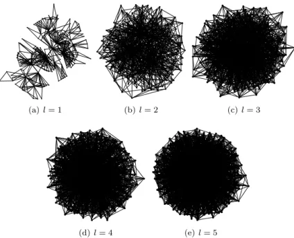
What is viewable in Figures 1 to 8 is basically that as l increases, the number of edges grows, and the graph takes a higher density. For the random cases (Figures 6 to 8) even with l = 1, it is possible to view a larger condensation than for the fixed size of the contexts (Figures 1 to 4). Part of this higher condensation is also observable in the value of the clustering coefficient, as we will see in the next section.

The Erd˝os-R´enyi graph is presented only in one figure due to the length of the stable sequence not be applicable for this case. There is only a difference in the amount of edges in the comparison with Barab´asi-Albert simulations with diffent values of l.

3.2 The Clustering Coefficient

3.2.1 First step

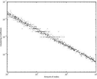
The first analyzed case is for k = 2, 3, 4, 5, l = 1, 2, 3, 4, 5 and t = 1. Figures from 9 to 28 show the CC in function of the number of nodes of the cases.

For k = 2 (emulation of the Barab´asi-Albert case), as expected, the CC vanishes as the number of nodes increases, even if l grows (it takes low levels slowly). There still are some artefacts in the simulations which seems not to be a property of the graph, but just a side effect of the estimation of the CC. The same problem appears for the larger graphs (next paragraph), but are already less significant due to the use of the function of the Figure 74 which determines the initial number of iterations in function of the number of edges to calculate the CC.

The value k = 3 is the first for which the theory from Gustedt [2008] proves a lower bound on CC. When l = 1 it is possible to see the CC stabilizing around 0.1 as the number of vertices grows. But for l = 2, we have a curve with higher values (but also stabilizes for larger graphs) and for l = 3 to l = 5, the curve goes down (always stabilizing in a specific value).

(14)

The general fact of the CC decreases as l grows can be a result of the boost of new neighbors of the new vertices in the context without a proportional number of new edges to connect the new neighborhood.

For k = 4 and k = 5, we have the same behavior, except that we do not have the higher curve for l = 2.

As described in section 2, we have used the amount of edges found in Barab´asi-Albert simulations for l = 1, 2, 3, 4, 5 for the emulation of Erd˝os-R´enyi model. In fact, we have five cases, which are different only in the number of edges of the graph.

The probability of connection between two vertices is equal to 2.l/(n + 1), where n is the number of vertices in the graph, which has a range from 1000 (probability approximately 2−3_{) to 1000000 (probability approximately 2}−6_).

We do not have a length of stable subsequences, but we have used all the different values of l (l = 1, 2, 3, 4, 5) of the Barab´asi-Albert simulations, which give us five different values for l in the expression of the probability of connection between two vertices.

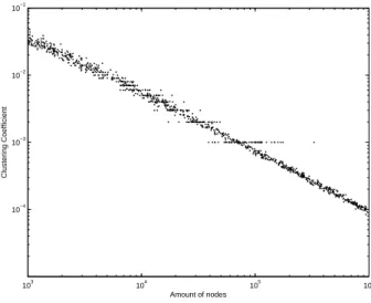
3.2.2 Larger graphs

Simulations for larger graphs was also done to verify if the results found in the previous are still valid.

There was a limitation for the simulations due to the machine where the program was running. Therefore, the unique case possible to run is those one with length of stable sequence l = 1.

It is valid to note the number of iterations used in this case, which is accord-ing the function presented at the end of the section 2.

The simulated cases was for the sizes k = 2, 3, 4, 5, l = 1 with the intersection between a new generated context and the old one which it is connected is Si=

k − 1.

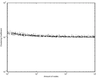
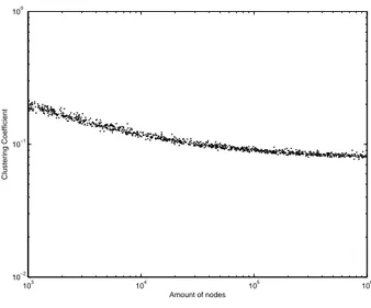
In Figures 34 to 37 we have the CC in function of the number of nodes of the graph. As expected, for the case with k = 2 (emulation of the Barab´asi-Albert case) the CC vanishes as the number of nodes grows.

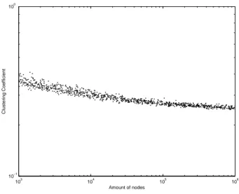
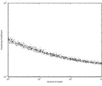
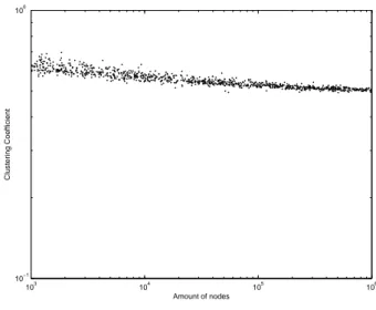
For the other sizes, the CC maintains “almost” constant even for graph larger than 106 _{nodes and it increases as k grows.}

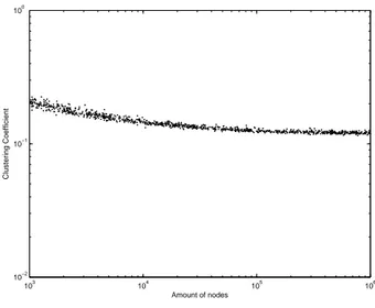
3.2.3 Graphs with random size of contexts

In this subsection, it is presented the graphs with random sizes of the contexts, as described in subsection 2.3.3.

Figures 38 to 52 shows the CC in function of the number of vertices in the graph for the cases of random sizes with two possible values (3 − 4, 4 − 5 and 5 − 6), for l = 1, 2, 3, 4, 5. An initial analysis demonstrates a decrease behavior of the CC as the number of vertices in the graph grows.

Figures 53 to 57 mixes the three cases and plots in the same figure the CC in function of the average size of the contexts in the graph, for l = 1, 2, 3, 4, 5. There is a viewable increase in the CC as the average size grows, with higher values for larger l.

The simulations of the other case of random sizes (predefined probability of happen a specific size) is illustrated in Figures 58 to 62. What is observable from these graphs is that even for larger graphs, the CC tends to maintain a

(15)

constant value. Moreover, the decrease from the initial value (with 1000 nodes) is higher for bigger l, and the curve of CC has larger values as big is l.

3.2.4 Comparing the results

In this section, regressions of the presented cases are done to compare the results for the different simulated parameters in the same figure. For each case, a fitted function for the points is used to plot some cases in just one picture to make easier the visualization of the results as their analysis.

The first case is the constant size of contexts simulated from 103 _{to 10}6

vertices. In Figures 63 to 66 we have the CC for the sizes k = 2, 3, 4, 5 and each case has the curves of l = 1, 2, 3, 4, 5. It is easily viewable that except for the cases of Barab´asi-Albert (k = 2) and k = 3, l = 2 the curve of CC tends to be lower as l increases. Moreover, except for Barab´asi-Albert, the CC seems to stabilize even for larger graphs.

The comparison between the sizes can be viewable in Figure 68, which has the results of the simulations with graphs from 103 _{to 10}7_{, k = 2, 3, 4, 5 and}

l = 1. The graphic emphasizes the vanish of CC for Barab´asi-Albert, otherwise, the cases k = 3, 4, 5 maintains the CC even for larger graphs.

The first random size of contexts case analyzed is that one with two possible cases in a graph. Figures 69 to 71 (3 − 4, 4 − 5 and 5 − 6 cases) shows the CC curves for l = 1, 2, 3, 4, 5. In all the cases, the CC is relatively high, but decreases as the number of vertices in the graph grows. The curve of CC is also higher for bigger sizes of the context and decreases as the length of the stable sequence decreases. Moreover, for all cases, it is viewable that the curves for higher l tends to a saturated curve which seems that even if we increase l, the curve will not change so much.

Figure 72 mixes the three cases and plots CC in function of the average size of the contexts for l = 1, 2, 3, 4, 5. For l = 1 and l = 2 the CC maintains almost constant as the number of nodes increases. But for l = 3, 4, 5, there is a little decrease in the value of CC as the number of nodes grows, stabilizing around 105_{nodes, which seems to have a little increase until 10}6_.

In the constant size of the context, for k = 2, due to the curve formed by the points liken a line in a log-log scale, the function f (x) = 10(b.log10(x)+c) _was

used to fit the points. For k = 3, 4, 5, due to the line be similar to a exponencial decrease, the function f (x) = 10(e(c.log10(x))+d.log10(x)+f ) _{(where e is the Euler}

constant) was used.

For the random case with two possible values for the context, the function which best fitted was f (x) = 10(e(c.log10(x))+d)_{. For the random case with}

prede-fined probability of each size, f (x) = 10(e(c.log10(x))+d.log10(x)+f )_.

For the graph of the clustering coefficient in function of the average size of the context, it was difficult to find a good function, therefore, that one which best fitted the points was

f (x) = 10(b.log10(log10(x))+c.log10(x)+d.(1−e(log10(x)))+f )_.

3.2.5 Execution time

To have an idea about the execution time to prepare the graph, and afterward to calculate the CC, some plots are presented.

(16)

Figures 75 to 94 show some cases of plots to understand how the parameters of the graph affects the computation of the graph and clustering coefficient. To prepare graph, i.e. to generate the graph with required number of nodes, the time grows quickly in function of the number of vertices in the graph, and the curve of the time ascends if l grows (there is more edges for larger l). The size of the context also dislocates the curve up.

Concerning the CC, all the printed cases have a similar behavior in the time to calculate the CC, except the k = 2 and Erd˝os-R´enyi cases. In general, for more edges in the graph, more time to calculate the CC is required.

4 Conclusions

In an effort to study a new network generation model, many simulations have been done. The model presented in Section 2 is more complex than some well knows network models in your structure, but is also quite simple to understand to generate larger graphs.

One of the observed point of this model is its capacity to maintain the clustering coefficient near a specific range of values even for larger graphs, ap-proximating natural networks.

Basically, two parameters of the model were analyzed in this report: the size of the context (basic unity of our model defined in Section 2) and the length of the stable sequence to add vertices in the graph (also defined in Section 2). For the size of the context, as larger it is, higher is the clustering coefficient of the network (it vanishes for k = 2, as expected, due to be the Barab´asi-Albert model or to be the Erd˝os-R´enyi model), and for length of the stable sequence, we have a decrease in the clustering coefficient as it grows. As discussed in the text, it can happen because the bigger neighborhood of a vertex when it links with more contexts diffused in the graph.

Another fact reported was the higher values of clustering coefficient with random sizes of the contexts instead of that one with constant sizes. For small graphs, the random size model with two possible values in the graph has a higher clustering coefficient, but for larger graphs, this model can not maintain this value, which decreases, and the model of random size with predefined probability for each size (total: 10 values of sizes) is more successful and has a higher clustering coefficient.

5 Acknowledgments

In this document, we report the work which has been done during the internship financed via the international internship program INRIA, under the supervision of Jens Gustedt.

Pedro Schimit was supported by EGIDE during this research and is grateful for the help and support of Jens Gustedt.

(17)

References

Albert-László Barabási and Réka Albert. Emergence of scaling in random net-works. Science, 286:509–512, 1999.

P. Erd˝os and A. R´enyi. On the evolution of random graphs. Madyar Tnd. Akad. Mat. Kut. Int. K˝ozl., 6:17–61, 1960.

graphviz. Graphviz - graph visualization software, 2008. URL http://www. graphviz.org.

Jens Gustedt. Generalized attachment models for the genesis of graphs with high clustering coefficient. Rapport de recherche, INRIA, 2008. URL http: //hal.inria.fr/inria-00312059/en/.

M. E. J. Newman. Scientific collaboration networks. i. network construction and fundamental results. Physical Review E, (64):016131.1–016131.8, 2001. Thomas Schank and Dorothea Wagner. Approximating clustering coefficient

(18)

Appendix

List of Figures

1 Graphical view of the graphs for k = 2 . . . 21

5 Graphical view of the graph for the Erd˝os-R´enyi model . . . 23

6 Graphical view of the graphs for random size of the context with k = 3 or k = 4 and varying l . . . 23

7 Graphical view of the graphs for random size of the context with k = 4 or k = 5 . . . 24

8 Graphical view of the graphs with prescribed context size distri-bution as for the co-author graph, see Newman [2001]. . . 24

9 Clustering coefficient in function of the number of nodes of a graph for k = 2, Si= 1 and l = 1 . . . 25

(20)

29 Clustering coefficient in function of the number of nodes of a graph for Erd˝os-R´enyi model with the same number of edges of the case Barab´asi-Albert with l = 1 . . . 35 30 Clustering coefficient in function of the number of nodes of a

graph for Erd˝os-R´enyi model with the same number of edges of the case Barab´asi-Albert with l = 2 . . . 35 31 Clustering coefficient in function of the number of nodes of a

graph for k = 2, Si= 1 and l = 1 . . . 38

38 Clustering coefficient in function of the number of nodes of a graph for random size of context varying between 3 and 4 and l = 1 40 39 Clustering coefficient in function of the number of nodes of a

graph for random size of context varying between 3 and 4 and l = 2 40 40 Clustering coefficient in function of the number of nodes of a

(21)

49 Clustering coefficient in function of the number of nodes of a graph for random size of context varying between 5 and 6 and l = 2 46 50 Clustering coefficient in function of the number of nodes of a

graph for random size of context varying between 5 and 6 and l = 5 48 53 Clustering coefficient in function of the average size of the

con-texts for random size (mixed the three cases) with l = 1 . . . 49 54 Clustering coefficient in function of the average size of the

con-texts for random size (mixed the three cases) with l = 5 . . . 51 58 Clustering coefficient in function of the number of nodes of a

graph for random size of context according to prescribed proba-bility of each size and l = 1 . . . 52 59 Clustering coefficient in function of the number of nodes of a

graph for random size of context according to prescribed proba-bility of each size and l = 5 . . . 54 63 Regression of the clustering coefficient in function of the number

of nodes of a graph for the case k = 2, Si= 1 and l = 1, 2, 3, 4, 5 55

64 Regression of the clustering coefficient in function of the number of nodes of a graph for the case k = 3, Si= 2 and l = 1, 2, 3, 4, 5 55

67 Regression of the clustering coefficient in function of the number of nodes of a graph for Erd˝os-R´enyi model with the number of edges equal to the number of edges of the Barab´asi-Albert simu-lations from l = 1 to l = 5 . . . 57 68 Regression of the clustering coefficient in function of the number

of nodes of a graph for the cases k = 2/Si = 1, k = 3/Si = 2,

(22)

69 Regression of the clustering coefficient in function of the number of nodes of a graph for random size of context varying between 3 and 4 and l = 1, 2, 3, 4, 5 . . . 58 70 Regression of the clustering coefficient in function of the number

of nodes of a graph for random size of context varying between 4 and 5 and l = 1, 2, 3, 4, 5 . . . 59 71 Regression of the clustering coefficient in function of the number

of nodes of a graph for random size of context varying between 5 and 6 and l = 1, 2, 3, 4, 5 . . . 59 72 Regressions of the clustering coefficient in function of the average

size of the contexts for random size (mixed the three cases) and l = 1, 2, 3, 4, 5 . . . 60 73 Regression of the clustering coefficient in function of the number

of nodes of a graph according to prescribed probability of each size and l = 1, 2, 3, 4, 5 . . . 60 74 Factor of multiplication to the number of edges of a graph to

obtain the initial amount of iterations for the calculation of the clustering coefficient of a graph . . . 61 75 Execution time to prepare the graph in the constant size of the

context case for k = 2, Si= 1 and l = 1 . . . 62

76 Execution time to prepare the graph in the constant size of the context case for k = 2, Si= 1 and l = 5 . . . 62

79 Execution time to prepare the graph in the Erd˝os-Rényi case for the number of edges equal to the number of edges of the Barabási-Albert simulations with l = 1 . . . 64 80 Execution time to prepare the graph in the Erd˝os-Rényi case for

the number of edges equal to the number of edges of the Barab´asi-Albert simulations with l = 5 . . . 64 81 Execution time to prepare the graph in the random size of the

context case with two possible values (4 and 5) for l = 1 . . . 65 82 Execution time to prepare the graph in the random size of the

context case with two possible values (4 and 5) for l = 5 . . . 65 83 Execution time to prepare the graph in the case with prescribed

probability of each size of context for l = 1 . . . 66 84 Execution time to prepare the graph in the case with prescribed

probability of each size of context for l = 5 . . . 66 85 Execution time to calculate the clustering coefficient in the

con-stant size of the context case for k = 2, Si = 1 and l = 1 . . . 67

86 Execution time to calculate the clustering coefficient in the con-stant size of the context case for k = 2, Si = 1 and l = 5 . . . 67

(23)

89 Execution time to calculate the clustering coefficient in the Erd˝os-R´enyi case for the number of edges equal to the number of edges of the Barab´asi-Albert simulations with l = 1 . . . 69 90 Execution time to calculate the clustering coefficient in the

Erd˝os-R´enyi case for the number of edges equal to the number of edges of the Barab´asi-Albert simulations with l = 5 . . . 69 91 Execution time to calculate the clustering coefficient in the

ran-dom size of the context case with two possible values (4 and 5) for l = 1 . . . 70 92 Execution time to calculate the clustering coefficient in the

ran-dom size of the context case with two possible values (4 and 5) for l = 5 . . . 70 93 Execution time to calculate the clustering coefficient in the case

with prescribed probability of each size of context for l = 1 . . . 71 94 Execution time to calculate the clustering coefficient in the case

(24)

A

Generated Graphs

(a) l = 1 (b) l = 2 (c) l = 3

(d) l = 4 (e) l = 5

Figure 1: Graphical view of the graphs for k = 2

(a) l = 1 (b) l = 2 (c) l = 3

(d) l = 4 (e) l = 5

(25)

(a) l = 1 (b) l = 2 (c) l = 3

(d) l = 4 (e) l = 5

Figure 3: Graphical view of the graphs for k = 4

(a) l = 1 (b) l = 2 (c) l = 3

(d) l = 4 (e) l = 5

(26)

Figure 5: Graphical view of the graph for the Erd˝os-R´enyi model

(a) l = 1 (b) l = 2 (c) l = 3

(d) l = 4 (e) l = 5

Figure 6: Graphical view of the graphs for random size of the context with k = 3 or k = 4 and varying l

(27)

(a) l = 1 (b) l = 2 (c) l = 3

(d) l = 4 (e) l = 5

Figure 7: Graphical view of the graphs for random size of the context with k = 4 or k = 5

(a) l = 1 (b) l = 2 (c) l = 3

(d) l = 4 (e) l = 5

Figure 8: Graphical view of the graphs with prescribed context size distribution as for the co-author graph, see Newman [2001].

(28)

B

The Evolution of the Clustering Coefficient

B.1 Constant Context Sizes

103 104 105 106 10−4 10−3 10−2 10−1 Amount of nodes Clustering Coefficient

Figure 9: Clustering coefficient in function of the number of nodes of a graph for k = 2, Si= 1 and l = 1 103 104 105 106 10−4 10−3 10−2 10−1 Amount of nodes Clustering Coefficient

Figure 10: Clustering coefficient in function of the number of nodes of a graph for k = 2, Si= 1 and l = 2

(29)

Figure 11: Clustering coefficient in function of the number of nodes of a graph for k = 2, Si= 1 and l = 3 103 104 105 106 10−4 10−3 10−2 10−1 Amount of nodes Clustering Coefficient

(30)

Figure 13: Clustering coefficient in function of the number of nodes of a graph for k = 2, Si= 1 and l = 5 103 104 105 106 10−2 10−1 100 Amount of nodes Clustering Coefficient

(31)

103 104 105 106 10−2 10−1 100 Amount of nodes Clustering Coefficient

(32)

(33)

103 104 105 106 10−1

100

Amount of nodes

Clustering Coefficient

Figure 19: Clustering coefficient in function of the number of nodes of a graph for k = 4, Si= 3 and l = 1 103 104 105 106 10−1 100 Amount of nodes Clustering Coefficient

(34)

103 104 105 106 10−1

100

Amount of nodes

(35)

103 104 105 106 10−1

100

Amount of nodes

(36)

103 104 105 106 10−1 100 Amount of nodes Clustering Coefficient

(37)

103 104 105 106 10−1

100

Amount of nodes

(38)

103 104 105 106 10−6 10−5 10−4 10−3 10−2 10−1 100 Amount of nodes Clustering Coefficient

Figure 29: Clustering coefficient in function of the number of nodes of a graph for Erd˝os-R´enyi model with the same number of edges of the case Barab´ asi-Albert with l = 1 103 104 105 106 10−6 10−5 10−4 10−3 10−2 10−1 100 Amount of nodes Clustering Coefficient

Figure 30: Clustering coefficient in function of the number of nodes of a graph for Erd˝os-R´enyi model with the same number of edges of the case Barab´ asi-Albert with l = 2

(39)

Figure 31: Clustering coefficient in function of the number of nodes of a graph for Erd˝os-R´enyi model with the same number of edges of the case Barab´asi-Albert with l = 3 103 104 105 106 10−6 10−5 10−4 10−3 10−2 10−1 100 Amount of nodes Clustering Coefficient

Figure 32: Clustering coefficient in function of the number of nodes of a graph for Erd˝os-R´enyi model with the same number of edges of the case Barab´asi-Albert with l = 4

(40)

Figure 33: Clustering coefficient in function of the number of nodes of a graph for Erd˝os-R´enyi model with the same number of edges of the case Barab´ asi-Albert with l = 5

(41)

103 104 105 106 107 10−6 10−5 10−4 10−3 10−2 10−1 Amount of nodes Clustering Coefficient

Figure 34: Clustering coefficient in function of the number of nodes of a graph for k = 2, Si= 1 and l = 1 103 104 105 106 107 10−2 10−1 100 Amount of nodes Clustering Coefficient

(42)

103 104 105 106 107 10−1 100 Amount of nodes Clustering Coefficient

Figure 36: Clustering coefficient in function of the number of nodes of a graph for k = 4, Si= 3 and l = 1 103 104 105 106 107 10−1 100 Amount of nodes Clustering Coefficient

(43)

B.2 Varying Context Sizes

Figure 38: Clustering coefficient in function of the number of nodes of a graph for random size of context varying between 3 and 4 and l = 1

(44)

(45)

(46)

(47)

(48)

(49)

103 104 105 106 10−1

100

Amount of nodes

103 104 105 106

10−1 100

Amount of nodes

(50)

103 104 105 106 10−1

100

Amount of nodes

103 104 105 106

10−1 100

Amount of nodes

(51)

103 104 105 106 10−1

100

Amount of nodes

(52)

B.3 Contexts with a Fixed Average Size

3 3.5 4 4.5 5 5.5 6

10−2

10−1

100

Average size of the contexts

Figure 53: Clustering coefficient in function of the average size of the contexts for random size (mixed the three cases) with l = 1

3 3.5 4 4.5 5 5.5 6

10−2 10−1 100

(53)

3 3.5 4 4.5 5 5.5 6 10−2

10−1

100

3 3.5 4 4.5 5 5.5 6

10−2 10−1 100

(54)

3 3.5 4 4.5 5 5.5 6 10−2

10−1

100

(55)

B.4 Context Sizes with Prescribed Probabilities

103 ₁₀4 ₁₀5 ₁₀6 10−2 10−1 100 Amount of nodes Clustering Coefficient

Figure 58: Clustering coefficient in function of the number of nodes of a graph for random size of context according to prescribed probability of each size and l = 1 103 104 105 106 10−2 10−1 100 Amount of nodes Clustering Coefficient

Figure 59: Clustering coefficient in function of the number of nodes of a graph for random size of context according to prescribed probability of each size and l = 2

(56)

Figure 60: Clustering coefficient in function of the number of nodes of a graph for random size of context according to prescribed probability of each size and l = 3 103 104 105 106 10−2 10−1 100 Amount of nodes Clustering Coefficient

(57)

(58)

C

Regressions for the Clustering Coefficient

Figure 63: Regression of the clustering coefficient in function of the number of nodes of a graph for the case k = 2, Si= 1 and l = 1, 2, 3, 4, 5

(59)

(60)

103 104 105 106 10−6 10−5 10−4 10−3 10−2 10−1 Vertice Clustering Coefficient l=1 l=2 l=3 l=4 l=5

Figure 67: Regression of the clustering coefficient in function of the number of nodes of a graph for Erd˝os-R´enyi model with the number of edges equal to the number of edges of the Barab´asi-Albert simulations from l = 1 to l = 5

(61)

Figure 68: Regression of the clustering coefficient in function of the number of nodes of a graph for the cases k = 2/Si = 1, k = 3/Si = 2, k = 4/Si = 3,

k = 5/Si= 4 and l = 1 - larger graph

Figure 69: Regression of the clustering coefficient in function of the number of nodes of a graph for random size of context varying between 3 and 4 and l = 1, 2, 3, 4, 5

(62)

(63)

Figure 72: Regressions of the clustering coefficient in function of the average size of the contexts for random size (mixed the three cases) and l = 1, 2, 3, 4, 5

Figure 73: Regression of the clustering coefficient in function of the number of nodes of a graph according to prescribed probability of each size and l = 1, 2, 3, 4, 5

(64)

D

Computing the Estimation of the Clustering

Coefficient

D.1 Number of Iterations

103 104 105 106 107 0 5 10 15 20 25 30 35 40 45 Number of edges

Number of times of the number of edges for iterations to CC

Figure 74: Factor of multiplication to the number of edges of a graph to obtain the initial amount of iterations for the calculation of the clustering coefficient of a graph

(65)

D.2 Running Times

103 104 105 106 10−3 10−2 10−1 100 101 Vertices

Execution time to prepare the graph (in seconds)

Figure 75: Execution time to prepare the graph in the constant size of the context case for k = 2, Si= 1 and l = 1

103 104 105 106 10−3 10−2 10−1 100 101 Vertices

(66)

103 104 105 106 10−3 10−2 10−1 100 101 Vertices

103 104 105 106 10−2 10−1 100 101 102 Vertices

(67)

103 104 105 106 10−3 10−2 10−1 100 101 Vertices

Figure 79: Execution time to prepare the graph in the Erd˝os-R´enyi case for the number of edges equal to the number of edges of the Barab´asi-Albert simulations with l = 1 103 104 105 106 10−2 10−1 100 101 102 Vertices

Figure 80: Execution time to prepare the graph in the Erd˝os-R´enyi case for the number of edges equal to the number of edges of the Barab´asi-Albert simulations with l = 5

(68)

103 104 105 106 10−3 10−2 10−1 100 101 Vertices

Figure 81: Execution time to prepare the graph in the random size of the context case with two possible values (4 and 5) for l = 1

103 104 105 106 10−2 10−1 100 101 102 Vertices

Figure 82: Execution time to prepare the graph in the random size of the context case with two possible values (4 and 5) for l = 5

(69)

103 104 105 106 10−3 10−2 10−1 100 101 Vertices

Figure 83: Execution time to prepare the graph in the case with prescribed probability of each size of context for l = 1

103 104 105 106 10−2 10−1 100 101 102 Vertices

Figure 84: Execution time to prepare the graph in the case with prescribed probability of each size of context for l = 5

(70)

103 104 105 106 10−3 10−2 10−1 100 101 102 Vertices

Execution time to calculate the CC (in seconds)

Figure 85: Execution time to calculate the clustering coefficient in the constant size of the context case for k = 2, Si= 1 and l = 1

103 104 105 106 10−3 10−2 10−1 100 101 102 Vertices

(71)

103 104 105 106 10−3 10−2 10−1 100 101 102 Vertices

(72)

103 104 105 106 10−3 10−2 10−1 100 101 102 103 104 Vertices

Figure 89: Execution time to calculate the clustering coefficient in the Erd˝os-R´enyi case for the number of edges equal to the number of edges of the Barab´asi-Albert simulations with l = 1

103 104 105 106 10−3 10−2 10−1 100 101 102 103 104 Vertices

Figure 90: Execution time to calculate the clustering coefficient in the Erd˝os-R´enyi case for the number of edges equal to the number of edges of the Barab´asi-Albert simulations with l = 5

(73)

103 104 105 106 10−3 10−2 10−1 100 101 102 Vertices

Figure 91: Execution time to calculate the clustering coefficient in the random size of the context case with two possible values (4 and 5) for l = 1

103 104 105 106 10−3 10−2 10−1 100 101 102 Vertices

Figure 92: Execution time to calculate the clustering coefficient in the random size of the context case with two possible values (4 and 5) for l = 5

(74)

103 104 105 106 10−3 10−2 10−1 100 101 102 Vertices

Figure 93: Execution time to calculate the clustering coefficient in the case with prescribed probability of each size of context for l = 1

103 104 105 106 10−3 10−2 10−1 100 101 102 Vertices

Figure 94: Execution time to calculate the clustering coefficient in the case with prescribed probability of each size of context for l = 5

(75)

615, rue du Jardin Botanique - BP 101 - 54602 Villers-lès-Nancy Cedex (France)

Centre de recherche INRIA Bordeaux – Sud Ouest : Domaine Universitaire - 351, cours de la Libération - 33405 Talence Cedex Centre de recherche INRIA Grenoble – Rhône-Alpes : 655, avenue de l’Europe - 38334 Montbonnot Saint-Ismier Centre de recherche INRIA Lille – Nord Europe : Parc Scientifique de la Haute Borne - 40, avenue Halley - 59650 Villeneuve d’Ascq

Centre de recherche INRIA Paris – Rocquencourt : Domaine de Voluceau - Rocquencourt - BP 105 - 78153 Le Chesnay Cedex Centre de recherche INRIA Rennes – Bretagne Atlantique : IRISA, Campus universitaire de Beaulieu - 35042 Rennes Cedex Centre de recherche INRIA Saclay – Île-de-France : Parc Orsay Université - ZAC des Vignes : 4, rue Jacques Monod - 91893 Orsay Cedex

Centre de recherche INRIA Sophia Antipolis – Méditerranée : 2004, route des Lucioles - BP 93 - 06902 Sophia Antipolis Cedex

Éditeur

Numerical results for generalized attachment models for the genesis of graphs

HAL Id: inria-00349461

https://hal.inria.fr/inria-00349461

Submitted on 31 Dec 2008

HAL is a multi-disciplinary open access

archive for the deposit and dissemination of

sci-entific research documents, whether they are

pub-lished or not. The documents may come from

teaching and research institutions in France or

L’archive ouverte pluridisciplinaire HAL, est

destinée au dépôt et à la diffusion de documents

scientifiques de niveau recherche, publiés ou non,

émanant des établissements d’enseignement et de

recherche français ou étrangers, des laboratoires

the genesis of graphs

Jens Gustedt, Pedro Schimit

To cite this version:

Jens Gustedt, Pedro Schimit. Numerical results for generalized attachment models for the genesis of

graphs. [Technical Report] RT-0361, INRIA. 2008, 74 p. �inria-00349461�

a p p o r t

t e c h n i q u e

Numerical results for generalized attachment models

for the genesis of graphs

Jens Gustedt — Pedro Schimit

N° 0361

models for the genesis of graphs

Jens Gustedt, Pedro Schimit

mod`

eles d’attachement pour la g´

en`

ese de

graphes

1

Introduction and Overview

2

Model

2.1

Objects and their Contexts, Gustedt [2008]

2.2

The generation of the graph

2.3

Variations and proposed simulations

3

Simulations results

3.1

A graphic view of the network

3.2

The Clustering Coefficient

4

Conclusions

5

Acknowledgments

References

Appendix

Contents

List of Figures

A

Generated Graphs

B

The Evolution of the Clustering Coefficient

B.1

Constant Context Sizes

B.2

Varying Context Sizes

B.3

Contexts with a Fixed Average Size

B.4

Context Sizes with Prescribed Probabilities

C

Regressions for the Clustering Coefficient

D

Computing the Estimation of the Clustering

Coefficient

D.1

Number of Iterations

D.2

Running Times