HAL Id: in2p3-00664324
http://hal.in2p3.fr/in2p3-00664324
Submitted on 30 Jan 2012
HAL is a multi-disciplinary open access
archive for the deposit and dissemination of
sci-entific research documents, whether they are
pub-lished or not. The documents may come from
teaching and research institutions in France or
abroad, or from public or private research centers.
L’archive ouverte pluridisciplinaire HAL, est
destinée au dépôt et à la diffusion de documents
scientifiques de niveau recherche, publiés ou non,
émanant des établissements d’enseignement et de
recherche français ou étrangers, des laboratoires
publics ou privés.
GALOPR, a beam transport program, with space-charge
and bunching
B. Bru
To cite this version:
B. Bru. GALOPR, a beam transport program, with space-charge and bunching. EPAC 88 - First
European Particle Accelerator Conference, Jun 1988, Rome, Italy. pp.660-662, 1988. �in2p3-00664324�
660
GALOPR, A BEAM TRANSPORT PROGRAM, WITH SPACE-CHARGE AND BUNCHING B. BRIJ
GANIL - B.P. 5027 - 14021 Caen Cedex - FRANCE
Abstract
GALOPR is a first order beam transport code including three dimensional space-charge forces and the beam ounching process. It deals with usual opticai devices (bending magnets, lenses, solenoids, drifts , bunchers) and can take into account any special optical device represented by its transfer matrix with space-charge the ("Miiller inflector" was recently introduced as one of these devices). The beam can be continuo%2s or undergoing a bunching or debunching process. The beam line parameters can be optimized in order to fit at will the 6 x 6 transfer matrix and the 6 x 6 covariance matrix for a maximum beam intensity. The results are presented with useful data tables and graphical displays.
1) Introduction
The computer code GALOPR (%NIL beam Lines Etics including Eadiofrequency bunchers) has been developed at GANIL from the code PRE1N.J (Ref. 1, 2! which was written at CERN to study the focusing and bunching characteristics of the Low Energy Beam Transport system
{LEBT) for the actual prc,ton linac injector, including space charge forces.
Firstly, a version without buncher but allowing to choose the ion mass number and charge state was used ai, GANIL to calculate the transfer lines between the 3 cyclotrons ; the space charge forces were taken into account in the dipoles.
Since 19r35, we have been developing the GALDPR version. Its universality makes it possible to calculate with linear approximation, the optics of a beam line ei.ther existing or being designed, for continuous or bunched beams, or beams in the process of being bunched, including space charge forces. Any buncher or rebuncher and any kind of element with an analytically known transfer matrix (drifts, quadrupoles, dipoles, solenoids) or a numerical transfer matrix are taken into account (Ref. 3).
The beam is considered as an hyperellipsoid in the 6 dimensional phase space. All forces, inclluding space charge are linear with respect to the reference partccle which in the present version is energy-fixed .
We have used GALOPR to study the axial injection beam line into the two injector cyclotrons for the GANIL modifications to come (0.A.E and 0.A.I) including a "Miiller inflector" in the 20 kV injection line and a "Pabot-Belmont inflector" in the 100 kV injection line. 2) Beam parameters
Each particle at a point S of the beam line LS located in the 6-dimensional phase space by its coordinates : x, x' = dx/ds, y, y' = dy/ds , z and z' = dz/ds, where s is the curvilinear coordinate. The fifth coordinate z is prcportional to the difference between the t:me of arrival of a particle at point S and the corresponding time to for the reference particle,
z = 'VP (t - to) (1) where vr is the velocily of the reference particle.
The beam is entirely defined by its intensity and the second order moments of the particle distribution in the 6-D phase space ; we will sometimes call these moments “rms” values”. They car. be written, for a centered distribution :
f u " P(V) dV - ."O
uv = f
with u,v E (x,x',y,y',z,z') "a
P(V) dV
(2)
where dV and V are -he volume element and the volume in the 6-D space.
If the 6 coordinates of each of the K particles of the distribution are known, the "rns" values become merelv :
- 1 N uv - ; f ui vi
(3) and define the covariance matrix x of the beam.
The type of distribution
iS
assumed to be hyperellipsoidal, i.e the surfaces of equal density are homothetic to the hyperellipsoid defined byC .If ci represents the envelope of the hype F
lipsoid for -;he coordinate u, then the ratio k = G 7 = fi/G is characteristic of the distribution. For an uniform distribution ( o= cstj in a n-D space, k =dx. A continuous beam, is represented by a infinitely long cylinder (n = 2, k = Z), and a bunched beam by an ellipsoid (n = 3, k = *, both being uniformly charged.
The rns emittanco in each of the 3 phase planes (x, x'), (y, y') and (z, z*) is given by :
--
L
(4)
ai>~i
is connected to the marginal emittanca by :ELI
= k* ;, (5) As demonstrated in Ref. 4, the evolution of the rms values depends mainly on the linear component of the space charge force, in the case of linear external forces. Therefore, all types of distributions having the same rms values can be treated by such linear programs ; the tuning of the physical parameters of the line is then the same for any distribution.The above-mentioned (cylinder and ellipsoid) have spare charge forces varying linearly with the coordinates and will be chosen in the following treatment as models.
3) Space charge force calculation
The components of the radial electric field inside an infinitely long cylinder with elliptical section are given by :
b a
E=-x x
a+b Ey - - a+b Y E, - C
i6) and inside an ellipsoid by :
=‘LJ.
X
P
Ex
t0EY
=-J,y t0 Ez =CJc z EO (7) wner’e a, b and c are the axes, if these volumes are in their principal axes, and where :EO = dielectric constant of vacuum s = space charge density
1
dx
Ja
==-abc 2(a" + X)(b' + X)(c2 + X) (S and analogous for J
P
and Jc are dimensionless elliptic integrals numerical y computed by the Gauss’ method.
Choosing s = vrt as the independact variable, the 4.3. Thick elements with coupled phase planes
equations of motion can be written f3r both models : We consider the most comolicated case of a dipole with the bunch tilted with respect to the axes: We first calculate the eigenvalues of the covariance matrix In the real space and the eigenvectors matrix (V) which transforms the (x, y, z) frame into the (x, Y, 7.) frame of the ellipsoid; the "rms" volue!.~
T‘i,;ii
,P of the ellipsoid are the above eigenvalues.d2x
e
- ds' - 2 E. (W/E) E, = K, x (9) and same for y and z
with W = energy per n~lcloon of t-he refe:ence particle. F: : charge to mass ratio.
introducing the rms values, we then get :
K; = P -ii for the cylinder
2 EIJ (W/E) ; + ; (same for y) Cl01
K: - P
2 E. (W/C) Jc for (same the ellipsoid for y, z) (11) 4) Transfer matrices ._
The beam line is composed of thick and thin elements ; the space charge forces act only in the thick ones, which are subdivised into steps, the length of which is chosen in such a way that it has only a small effect on the transverse dimensions.
We use 4 types of transfer matrices : 4.1. Thin elements
The t.ransfer matrix for a pole-face rotation :I?. one end of a dipole, and for a rotation of the transverse coordinate systet~ ari>l:nd tte ,:urvilinear coordinate are given in Ref. 5.
Any element (or comhinaison of elements) FE'-d;OUSiJr cnl~~l~lnt.aci and ,gi "PI-i in a ndncrical form
(for instance, the Pabot - Belmont inflector ) can he introduced in the program as a G X 6 matrix.
0.2. Thick elements with decoupled phase planes
If the reference frame of the ellipsoid anti of t.he motion are the same, then the space charge fzrccs {KC,) can be added to the external ones (O,J) in each phase plane, lea31nr: to the Hill.-rype equa?ion.
22.. =+(Q,-K,)u-0 ds2
'The following table glVl2S the constants Qu correspondi rig to the external forces of the different elements :
I
i Qx
/Drift Spdce/ 0! Qy
/ Qz
1
/:?/.?/ I BR = magnetic rigidityRX = distance between 2 consec,Jtive bunches adjacent G = quadrupole gradient (G ) 0 is focusing in the x
direction)
B : maxinum field in the solenoid
VET = maximum voltage times transit tine fact.or on the axis
k
= gap length for a single-gap element = solenoid length
('1 A rotation by an angle Q 1,s must be added afterwards to get the transfer zatrix in the initial reference frame.
In each plane, the 2 x 2 trarsfer matrix contains sine and cosine terms if Qu - Kt,> 0 and cash and sinh terms if Qu - KU < 0.
661
According to the previol;s paragraph, the space charge forces Kx, Kyand KZ can be calcxla~ed.
The new 6-D covariance matrix may be obtained in two ways.
1st. method
The 6-D covariance matrix is calculated in the (X, Y, 2) frame ; then, a new one is obtained by the action of a thin lens with a strength equivalent to the effect of the space charge force over one step.
This new matrix is projected on the original reference frame, and is finally transfered through the next element step.
2nd. method
The forces FXX, KyY and KZZ are projected on the original axes, glvln-7
F Fr, Fz
= [VI“ [):I K, K, j [“I El=&“]
j:]
113) :tese constants Ktju mllst SC added to the external l‘o~~r.~:: imp1 i tbti in tiip, rl:-iss~c:~l s;yatrm :
112 x 11 1 tlz -_ -x= -- ds2 P2 p ds
,I2 ”
--=-+
dsi’
Ly=Q
02
d*z 1 dx -a _-- ds2 P ds with II 7 f‘iald index(13) R = radius of curvature of the reference franc. And the resillting system is solved by classically going to a Runge-Kutta method applied to a six first-order differential equation system.
The final transfer matrix is composed of the 6 vectors, solutions of the system. It is however necessary to perform a matrix transformation at both ends in order to take into account the difference between entrance and output reference frames.
This second method is more time consuming but it is more physical to add all the forces before solving the equations.
4.4. Special eierrents
The Miiller inflector can be given as an example since it can he represented by an analytical matrix from the origin to any points inside it. Care of the space charge effect is taken by adding a perturbation matrix (Ref. 6). In GALCPR, we are only using the total transfer matrix (Ref. 6) for a 9:~~ deflection angle ; sir,ce an icflector is necessarily attached to the central region of a compact cyclotron, two additional factors mt:st be taken into account : the magnetic field variatinn along the trajectory and a rotation to match the reference frame of the accelerated mntion.
662
5. Transition from a continuous to a bunched beam. ,211 the elements studied above have a linear action on the beam. When a continuous beam, with a negligible energy spread traverses a buncher, the energy modulation resulting from the sinusoidal voltage generates a longitudinal emittance. In our model, it is of importance to include in this emit-tance only the particles that will be captilred further while taking intc account the effect of all the particles (including those which will be lost! for the space charge force calculations ; we proceed in 3 steps :
5.1. Generation of the longitudinal emittance at the buncher
Before the buncher, the emittance is a single line along the phase axis (zero energy spread). The relative momentum spread is given by :
SF
e VeT z'=.-=-- P 2 (W/E) sin (2 7T 3 bunchcr(151
longiludinal emittonce 2" +-c conhuour beam region of occeplcd Figure 1 porliclelThe assumption is that, at the buncher, the trapped particles lie inside the hatched region of figure 1 ; the separation between the trapped and rejected particles is called the "cut-off" phase @ .
Since, at this point, the beam is continuous: the trapped intensity is proportional to I$ :
i trap = i. a <:/ n where io is the curregt upstream. n = ec,'n is the "bunching efficiency“. In order to inject this ounch into the following sections of the line /the hatched portion of the cylinder is modified into an ellipsoid with the same volume and the same transverse rms values ? and y' . The rms valires are
calculated assuming an uniform distribution between -Qe and @ in the ellipsoid or between - Qc and $c in the cylinder (the z and 2'2 expressions are detailed in Ref 1, 2).
When several bunchers are present, the modulation is no longer a simple sine and it is much easier to
make a numerical treatment to calculate the modulation and therefore to ,calculate the rms val~les, which is the case in our computer code where a double drift harmonic buncher is considered.
5.2. Introduction of the space charge
We then have to fulfill the following requirement: there nust be continuity of the space charge forces during the transition from a 4-D to a 6-D phase space.
The chosen model is a combination of the actions of a infinite cylinder with the density p of the rejected particles and of an ellipsoid with th% density
P - p where c pa%ticleZ.
, is the density of the trapped These denzities are given by :
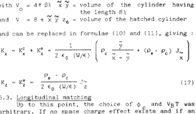
1, ' T PF ln T, i p --I-.-Lrl e V p, _ = v - v (1 - rl) 0 (16) with V = 0 4nar "xy= and V =en;yz,=
and can be replaced in 1 K zm KC + Ke ii
x x x 2 to (W/E)
K =Ke= z I I', - P, .:- 2 to (W/E) z
volume of the cylinder having the length 13)~
volume of the hatched cyiinder formulae (10) and (11). giving :
+ (P, - PC, J, x 1
(17) 5.3. Longitudinal matching
Up to this point, the choice of @ and VBT was
arbitrary. If no space charge effect exfsts and if an upright ellipse is required at the end of the line, the phase acceptance @ is given by the intersection of the ellipse with the aphase axis and depends only on 9, and not on VBT.
In the presence of space charge forces, one must use a minimization method acting on @c and VBT in order
to obtain the desired s, value. 6. General optimization
The previous sections show that it is possible to transport a beam with space charge forces along a beam line of given structure. The goal of the program is also to dezermine the tuning parameters of the elements in order for the beam to be matched, i.e. for its 6-D
omittance to fit the required acceptance.
In the transverse places, the main parameters are the quadrupole gradients (and rarely the drift lengths); they are varied in order to :
- fulfill given conditions on some elements either of the covariance matrix or of the transfer matrix at the matching point,
- limit the beam dimensions locally or along the whole Line.
In the longitudinal plane, the matching is possible by varying &, VBT of the first buncher and the voltage of a rebuncher.
Due to the various couplings between the transverse and longitudinal planes, all the parameters, conditions and limits are included in the same
optimization which is carried out by a least-squares method.
7. Conclusion
The code SALOPR is now ?unning onto the IBM 3C90 (VM/CMS system! of the CL IN2P3 IIN2P3 computer centre
in Lyon) and into the 32 bits MODCOMP at GANIL : an off-line code allows to drew the beam envelopes onto a
“BENSON” plotter.
Two further improvements to this code are planed
by introducing :
- a thin lens taking into account the space charge effects in an element whose transfer matrix is given in a numerical form,
- elements in which the central particle is accelerated.
References : ~-
(1) E. Bru and M. 'Weiss, CERN/MPS/LIN 72-4
(2) Y. Weiss, Proceeding of the Particle Conference San Francisco, 1973, IEEE NSZO, n020, no 3 (1973) p. 877 (3) B.BRU, GALOPR : Un programme de traIlsport de faisceau incluant la charge d'espace et le groupement, GANIL 68/16/TF/Ol
(4) F. Sacherer, CERN/S/DL/70-12
(5) K.L. Brown, D.C. Carey, Ch. Iselin and F. Rothacker, CERN/80-04
(6) R. Beck. B. Bru and Ch. Ricaud, L'inflecteur hyperboloidal de R.W. Miiller , GANIL A86-02 a et b.