Dynamical modeling of a micro
AUV in hydrodynamic ground effect
The MIT Faculty has made this article openly available.
Please share
how this access benefits you. Your story matters.
Citation
Bhattacharyya, S, AJ Reyes, and HH Asada. “Dynamical Modeling of
a Micro AUV in Hydrodynamic Ground Effect.” OCEANS 2016 MTS/
IEEE Monterey (September 2016).
As Published
http://dx.doi.org/10.1109/OCEANS.2016.7761326
Publisher
Institute of Electrical and Electronics Engineers (IEEE)
Version
Author's final manuscript
Citable link
http://hdl.handle.net/1721.1/118924
Terms of Use
Creative Commons Attribution-Noncommercial-Share Alike
Dynamical Modeling of a Micro AUV in Hydrodynamic Ground Effect
S Bhattacharyya
1AJ Reyes
2and HH Asada
3Abstract— The need for inspection of subsea infrastructures - ranging from ship hulls to pipelines - have led to development of various underwater vehicles specifically geared towards such missions. One such example is the EVIE (Ellipsoidal Vehicle for Inspection and Exploration) robot developed by the d’Arbeloff Laboratory at MIT, which is a water jet propelled ellipsoidal micro AUV with a flat bottom designed for scanning and moving on submerged surfaces. Near proximity to surfaces is important for using sensors like ultrasound for imaging internal cracks that cannot be done by simple visual inspection. However movement on submerged surfaces without wheels or tether is challenging since they are often rough due to rust or corrosion. The d’Arbeloff Laboratory has previously presented an extensive research on utilizing natural ground effect hydro-dynamics during longitudinal motion of the AUV to maintain a self stabilizing equilibrium height very close to the surface. Further, it was also demonstrated that using an active bottom jet we can form a stable fluid bed of thickness about 1/200 to 1/50 of the body length and enable smooth gliding of the robot on rough surface. Previous work presented has focussed on the observations, computational fluid dynamic (CDF) simulations of the phenomenon, analysis of the different regions of the ground effect force and some preliminary experimental results. In the research presented in this paper, we go one more step further and provide a deeper insight to the dynamical modeling of motion near a submerged surface and its dependency on design parameters. This is of particular relevance since understanding the system dynamics and response characteristics will enable us to design a control system which in turn can deal with the unusual near surface behavior of this underwater vehicle and help transition the design for more practical applications. The work here also substantially explores linearization techniques for this highly non linear system to enable traditional linear control and demonstrates methodologies of using experimental data for modeling purposes instead of a pure analytic model.
INTRODUCTION
Motion on or near proximity of submerged surfaces is becoming a subject of great relevance with the increasing number of subsea activities. Applications include but is not limited to ship hull scanning for searching hidden threats, scanning or imaging of sea floors, inspection of pipelines and oil rig infrastructure, underwater data cables monitoring for cyber security threats or identifying stealth mines [1] , [2], [3]. Often visual imaging is not enough- cause defects and threats may be hidden or are internal to the inspection
Work has been supported by the National Science Foundation, grant number NSF CMMI-1363391.
1S Bhattacharyya is a PhD Candidate at d’Arbeloff Laboratory in the
Department of Mechanical Engineering, [email protected]
2AJ Reyes is an undergraduate student in the Department of Mechanical
Engineering, MIT and a research assistant at d’Arbeloff Robotics Labora-tory, [email protected]
3HH Asada is the Ford Professor of Engineering and Director of
d’Arbeloff Laboratory for Information Systems and Technology, Department of Mechanical Engineering, [email protected]
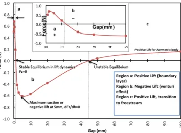
structure. Over last six years at MIT’s d’ Arbeloff Lab, our work focussed on simple ellipsoidal micro submersible (anywhere between 150mm-250mm in the long axis) or micro autonomous underwater vehicles (AUV) to perform these tasks as an alternative to using traditional ROVs and AUVs. Our latest design which is an ellipsoidal robot with a flat bottom, is capable of moving in multi DOF in the free stream as well as on surfaces underwater without wheels or tethers by simply using water jets for propulsion [4]. An overview is shown in Figure 1. However rust and corrosion causes movement on submerged surfaces difficult due to friction. In our previous research [5],[6] we found longitudi-nal motion near the vicinity of submerged surface creates a self stabilizing phenomenon (natural hydrodynamic ground effect) that allows the body to be on a stable equilibrium - i.e. resting on a thin film fluid (⇠ 1mm) while moving forward (note the same would happen for sideways motion). The ground effect force versus height curve from Ansys CFD simulation data is shown in Figure 2 for a robot moving at 0.5m/sec. If pushed above the stable point, a strong suction or “venturi force” brings the body back to the stable point and if pushed down to press on to on the surface, it experiences a repulsion force (note the early region of the curve) pushing it back to the same equilibrium again. This enables a non contact yet extreme close proximity inspection, thereby overcoming surface friction (within bounds) simply by using natural hydrodynamics.
However, though the concept was promising it could only be validated for extremely ideal situation in a tow tank- i.e. relatively calm water with little or no external turbulence. In the more recent research [7] we presented a design variation with a single impinging bottom jet as shown in Figure 3 and showed a similar self stabilizing phenomenon can also occurs for vertical motions as shown in Figure 4. The single axis underwater motion phenomenon demonstrated is analogous to an underwater “Vertical Take off and Landing” (VTOL) vehicle [8],[9]. When the body is very close to the surface with the jet impinging the ground (⇠ 5mm 25mm), intuitively one might be expecting a higher thrust force while pushing against the wall. Instead we experience a strong suction force, created due to wall effects and the formation of ground vortices as shown in Figure 3. This in case of a traditional Vertical Take Off and Landing Vehicle (VTOL) with downward impinging jet is referred as the “jet induced lift loss”. This is undesirable in aerial VTOL vehicles since it causes a noticeable lift reduction. Further, another unusual observation in our experiment is that, when the body underwater is put in contact with the horizontal surface and the jet is turned on, it is seen that instead of
Fig. 1. Top Left: Conceptual idea for submerged pipe inspection. Top Right: Conceptual prototype Bottom Left: Actual Prototype Bottom Right: Prototype moving on a surface in a 3ft deep tank using water jets for propulsion
Fig. 2. Lift force versus height for a flat bottom robot moving at 0.5m/sec in close proximity to the ground. Note natural hydrodynamics causes a stable equilibrium at ⇠ 1.5mm. The paper [6]explains the phenomenon in details
the body taking off vertically (assuming the net body weight
underwater, W < FT where FT is the thrust force from the
bottom jet), or even experiencing further suction, it simply releases the pressure build up from the bottom and sits on a thin water film. If you press down the body further down into this region, it will push back and stabilize once again on this fluid (water) film[10], [11]. We called this the “pressure build up region”- a phenomenon that can be compared to a fluid bearing. The third region which was discussed previously but not important for very close proximity inspection is the heights at which the body is able to stabilize or hover at reduced thrust using the upwash force from the surface created by the impinging downward jet. This is called the
Fig. 3. A block schematic showing the different effects of the ground with an impinging jet. The wall jets, ground vortex and fountain upwash phenomenon are shown here that leads to negative or positive lift
Fig. 4. The different regions of the ground force due to an impinging jet
“fountain upwash region”.
GROUNDEFFECTFORCEMODEL
In our research so far, we have demonstrated and ana-lyzed the hydrodynamic ground effect phenomenon - the different force regions- and their implications mainly through experiments and simulation. We have observed the effects of changing parameters like size or area of the body or noted how the flow changes by varying the underbody design [5]. In this paper, now take a deeper dive into modeling the system -particularly keeping in mind the need for an onboard control system. Some of the parameters taken into account for the modeling should be the characteristic gap, size and scale of the object, the height from the ground, the flow rate, velocity of the body, surface roughness among others.
From previous research presented, it was shown that the non dimensional lift force is dependent solely on the
characteristic height, that is e = h/c where h is the height
from the ground and c is the chord length of the body. It is observed that the ground force can be represented as a
function of height and the thrust force FT. The thrust force
FT goes quadratically as the velocity of the jet wj as well as
the pump control voltage V (direct control variable). That is,
Fg=f (h) f (V ) = f (h) f (FT) =f (h) f (wj) (1)
as-Fig. 5. CFD Fg data scaled by 1/wj2.
Fig. 6. Left: Shows the Fgfor all different voltages Right : Shows Fg/f (V )
to see the sole effect of distance. Unlike the CFD results, the curves do not overlay due to unaccounted factors in the experiment.
FT = ˙mewe ˙mowo+ (pe po)Ae (2)
where ˙m is the mass flow rate, and subscript e and o denote parameters at entrance and outlet of the nozzle. Again, the mass flow rate which is related to velocity as
w =rA˙m (3)
The CFD data of Fgoverlays perfectly as we scale byV12 '
1 w2
j - taking away the dependency on flowrate (or voltage or
velocity). So, the height dependency is given by the curve shown. We can say that,
Fg=f (FT)f (h) = q2f (h) (4)
The curve in Figure 5 shows Fg(h) = 1/q2F(g)- which
gives us a clear idea of how the force depends on the
height at a given FT and - as expected -is highly non linear.
The overlaying of the experimental data was not that clean since there are many other real parameters that affected the experiment came into play. This is seen in the Figure 6. Although it doesn’t overlay, the force is scaled down to a factor of ⇡10. The result could still be used for an initial
estimation for Fg when applying an estimation theory for
determining Fg.
Fig. 7. Experimental Setup for Roughness Test
Fig. 8. Ground Effect Force comparison between rough surface and smooth(glass) surface
In this paper for both experiment and CFD run - we simplify to using a elliptical plate of quarter inch thickness with a center outlet, since our interest is mostly about the hydrodynamics occurring at the bottom of this plate. For most of the work presented here, the upper body effect is not explored. The dependency on scale was explored. It was
found that the ground force Fg(h)µ A µ L2 where A is the
area of the body and L is the length.
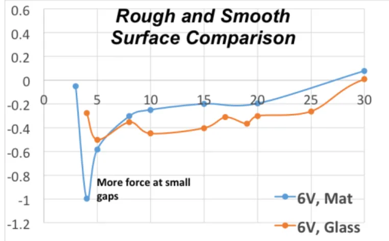
The next parameter of interest was surface roughness. In a lab experiment, we used a rough mat with roughness
factor er=dcr⇡.008, where dr is the height of the surface
roughness and c is the nozzle diameter. Intuitively one might think surface surface leads to turbulence in the flow, thereby would decrease the suction or venturi effect. It was seen from the experiments that in fact the suction became stronger at smaller gaps but decreased at larger gaps.This is because rough surfaces causes local vortices leading to increase in suction, or pressure drop dominant when closer to the surface. The setup is shown in Figure 7 and a comparison example with the given mat and just glass surface is shown in Figure 8.
To measure the forces, we conducted an experiment con-straining the body to only one degree of motion (Z) and used a single point 100g micro load cell. Sensors used are two kinds- a precision distance sensor and a larger distance sensor
Fig. 9. Left: Schematic showing experimental setup with elliptical plate. Right Top: Setup for Distance Measurement. The white plate moves with respect to the ultrasound sensor along with the elliptical plate. When the body touches the ground, the white plate is the furthest from the sensor (taken as positive distance). Right bottom: Pump mounted on elliptical plate resting at equilibrium
(ultrasonic distance with .05 mm accuracy). The force sensor is a 100gm micro load cell. Repeatability and hysteresis for this sensor is ⇡ .005N = 1/100 of the force measured. Setup shown in Figure 9. The sensor data is further filtered to get a precise estimation of the distance from the ground. Effects of other submerged portion subtracted out through subtraction of the value at no load (no pump). Error sources came from the friction in the slider , sensor measurements, limitations in reproducibility of the setup and inaccuracy in the system measurement.
SYSTEMRESPONSE
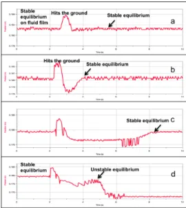
As mentioned, instead of using the whole robot, we used elliptical plates cut into the shapes of robot’s bottom. We looked into the effect of a sudden external force on the system with different buoyancy conditions pushing it all the way to the ground. The set up is shown in Figure 9. A ultrasound distance sensor was used in the arrangement shown to measure distance. Note, negative distance implies away from the ground.The system response is given byFigure 10.
THESYSTEMMODEL
Hydrodynamic force on a body in motion in the vicinity of a submerged surface is substantially different from motion in the free stream and is under-explored. The Fg(h) curve is unique and challenging to model - particularly due to the presence of multiple equilibria- one stable at very small distance and one unstable at a comparatively larger distance. The system dynamics is characterized by complex non linearities which are non monotonic in nature. Traditional linearization techniques though most preferable cannot cap-ture the behavior of the body in the entire near surface region of operation (about 1m for a body of comparable size to our robot), which limits on how we can model a linear controller for the same. Complex non linearities though command non linear modeling and control- it is interesting to explore data driven linearization via studying system performance and investigate possibility of using linear control by capturing
Fig. 10. (a) An force of 5N given. Very damped system, stabilizes right away on the fluid film (b)Body made slightly more buoyant- note the body bounces on the other side of the equilibrium into the venturi region and is sucked back to stability (c) Body is made even more buoyant - experiences lesser venturi force - oscillations representing possible lateral vibrations (d)Further increase in buoyancy shows for the same force - the body escapes the venturi region and passes through the unstable equilibrium to free stream region- flat section. (max distance allowed in the experiment)
the non linearities in what we call a “pseudo linear model”. We will explore this concept further in this section with some preliminary results.
The non linear model of the single axis vertical motion of the jet impinging robot can be given as
˙w = 1
Sz[(mg Fb) +Fg(u,h) + FD+Fj] (5)
˙h = w (6)
where, Fd, the drag force (if considered quadratic) is given
by Fd = Zwww2, and w is the vertical velocity of the robot or
plate. The non linear terms - Fgand FD- are major constrains
to linearize the above equations for constructing typical state space equations. For traditional linearization, we consider only the area of interest - up to the upper bound of the venturi or “suckdown” region. The simulation data is fitted into a quadratic functionas shown in 11 which is then linearized.
˙w = 1
Sz[(mg Fb) +uj[ah
2+b ⇤h+g]+Z
www|w|+uj] (7)
˙h = w (8)
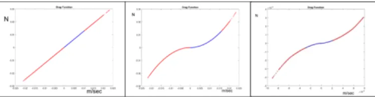
In the region of the operation, the drag function is complex- it is linear in very small gaps and slowly transitions to quadratic in larger gaps as shown in the Figure 12. For the same operation region, we show where the body would fall in a drag force versus velocity curve. Linear model works well if we constrain ourselves only to very small gaps , and quadratic for large types. For simplicity though quadratic drag works, mixed drag model represents a more ideal curve.
Fig. 11. Parabolic Fit in the region of Interest (Venturi Suckdown)
Fig. 12. Drag Types- Left: Linear Middle: Quadratic Right: Mixed
Here uj is the thrust control which regulates the thrust
force of the bottom jet Fj and goes quadratic as voltage V
or jet velocity wj.
The linearized parametric model for a quadratic drag type is given by ˙w ˙h = Zwwwe ue(2hea + b) 1 0 + 1 Sz 0 (9)
Let us now consider the equilibrium position, for a
con-stant uj=k, as the position of the stable height where Fg=0,
and remap it to h=0 by shifting the Fgcurve to pass through
(0,0). Here the parametric model is now linearized at the
equilibrium- that is - are we=0v/sec, h = 0m. When the
values are substituted in the Jacobian matrix of the state space model, the damping term disappears leading to the failure of the linear model.
˙w ˙h = 0 kb 1 0 + 1 Sz 0 (10)
The second alternative is a pseudo linear model, where we apriori have an estimate of the range of velocities the body can attain, and we use the RMS value of the velocity and that accounts for the damping. Or if the drag model is considered linear- but that constrains us to very small distances only (< +/ 3mm). The downside of the RMS method is a prior estimate of expected velocity is needed for pseudo linear model and also this model doesn’t cover the entire non linear region. ˙w ˙h = Z wwwrms kb 1 0 + 1 Sz 0 (11)
The performance is seen in the Figure 13. The linear model (blue) shows no damping, the modified linear or pseudo lin-ear model (red) shows a smooth convergence to equilibrium and the non linear model (black) simulation shows damped oscillations and eventual stabilization at equilibrium.
Fig. 13. Blue: Linear model Red: Modified Linear Black: Non linear ODE simulation results. Left: Velocity Right: Height
Given, there is no simple linear model to capture the non linearities, we explored the idea of using data, i.e. experimental or CFD simulation data of the system for coming up with a unique linear model that is capable of capturing nonlinearities. This is done by augmenting ”auxiliary variables” associated with the non linearities with the output vector. Since it is challenging to use usual statistical algorithms, we used a relatively new method of system identification, namely “subspace method” or 4SIDmethods (Subspace State Space Systems IDentification). This method is used for the identification of the linear time-invariant models in a state space form from the input-output data, which in our case comes from simulations and or lab experiments. Contrary to the ARX or ARMAX model, subspace method is based on geometric progression and linear algebra principles. There are various algorithms in the subspace method that can be used. We use N4sid in our case to find a linear latent variable model form that can have a possibility of using linear control. Some of the important work on the augmentation of auxiliary variables are shown in [12][13].The model is explained as below.
Let y represent the augmented output vector, and z 2 ¬nzis
the latent vector, ˜A 2 ¬nzxnz is the system matrix and ˜B 2
¬nzxm is the input matrix in latent space, and ˜C 2 ¬lzxnz is
the output matrix. We feed the algorithm with the known in-formation as output data- that is, the height, the velocity, the ground force and the drag force experiments (or simulation data). The input is the external input to excite the system over the region of operation. The equations below represents the formulation of an approximated linear dynamical model.
y = 2 6 6 4 h w Fg Fd 3 7 7 5 (12)
z(k + 1) = ˜Az(k) + ˜Bu(k)
y(k) = ˜Cz(k)
z(k) = ˜C 1y(k)
(13)
Now representing the state equation in terms of the output y we have
y(k + 1) = ˜C ˜A ˜C 1y(k) + ˜C ˜Bu(k) (14)
Renaming the variables to represent the above in a familiar state space model,
let-y = X Al= ˜C ˜A ˜C 1 Bl= ˜C ˜B X(k + 1) = AlX(k) + Blu(k) Y (k) = ClX(k) (15)
The system is now represented in a higher dimensional space as a linear model. However the real second order system, in actuality can only measure height and velocity when in free motion. To see if we can estimate the unknown non linear auxiliary variables of interests from an estimator by simply feeding back the error from the actual model measurements into the higher dimensional model, we use a state observer (Luenberger Observer) [14]. In this case, our
Cl matrix now looks like:
Cl=
1 0 0 0
0 1 0 0 (16)
The observer equation for estimating the state and auxil-iary variables are then given as
ˆX(k +1) = AlˆX(k)+Blu(k) + L(Y (k) ˆY(k))
ˆY(k) = ClˆX(k) (17)
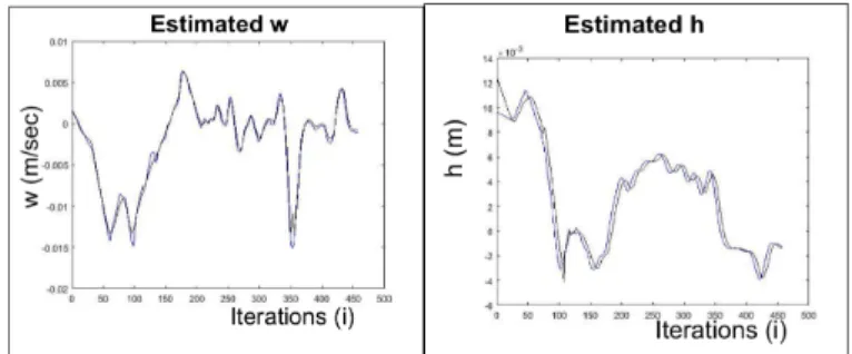
Following are some of the preliminary. The Figure 14 shows estimated height and velocity, when fed with real experimental input and output measured data- where the system was pushed down to the surface and released. We then show the estimated(red) forces - the ground force and the drag force and compare it with the measured ones (blue) as shown in Figure 15. Note the approximated model’s matrices unlike traditional state space system matrices are not insightful, rather a result of a black box model. The matrices are estimated such that the output data matches the data fed into the algorithm. Therefore this does make traditional system matrix analysis challenging from simply looking at the data driven state space model.
Fig. 14. Left: Estimated Velocity(blue) and measured (black) Right: Estimated height (blue) and measured (black)
Fig. 15. Left: Estimated Fg(blue) and measured (red) Right: Estimated Fd (blue) and from experiment (red)
CONCLUSION
The paper presents insights on system dynamics and modeling of a micro AUV in hydrodynamic ground effect. This work is unique and new since dynamics of a body moving near a submerged surface is not well explored. We demonstrate dependencies on different parameters as well as system response to external perturbations. We then proceed to develop a model appropriate for a control system. We show that the effect of hydrodynamic ground effect is highly non linear and traditional linearization cannot incorporate the features of the entire operational region. Yet, since linearized model would simplify the control system for real world implementation, therefore we explored the idea of data driven model with auxiliary variables in an augmented output vector and showed some preliminary results. The abundance of cheap sensors and ease of taking data makes this a viable approach. We used subspace method for developing the state space model in the latent variable space. However, we found though subspace methods like N4sid can give results better than traditional linearization, we had little insight into the state matrices and it required the right combination of many tuning variables. That is, the combination of parameters to optimize in subspace methods can be extremely complex to understand intuitively. However considering small mi-cro AUVs with unconventional design and mission plans can have an important impact in the future of underwater robotics, thorough understanding of system dynamics is crucial and we will continue to explore new reliable methods of using historical data from sensor or simulation that will enable us to capture a wider range of operational region.
REFERENCES
[1] J. Vaganay, M. Elkins, D Esposito; W. O’Halloran; F. Hover.; M. Kokko “Ship Hull Inspection with the HAUV: US Navy and NATO Demonstrations Results”, OCEANS 2006 , vol., no., pp.1,6, 18-21 Sept. 2006
[2] K. Asakawa, J. Kojima, Y. Ito, S. Takagi, Y. Shirasaki, N. Kato, “Autonomous Underwater Vehicle AQUA EXPLORER 1000 for In-spection of Underwater Cables”, Proc. of the 1996 IEEE Symposium on Autonomous Underwater Vehicle Technology, 1996, pp 10-17. [3] Hougen, D.F.; Benjaafar, S.; Bonney, J.C.; Budenske, J.R.; Dvorak,
M.; Gini, M.; French, H.; Krantz, D.G.; Li, P.Y.; Malver, F.; Nelson, B.; Papanikolopoulos, N.; Rybski, P.E.; Stoeter, S.A.; Voyles, R.; Yesin, K.B., “A miniature robotic system for reconnaissance and surveillance”, Robotics and Automation, 2000. Proceedings. ICRA IEEE International Conference on , vol.1, no., pp.501,507 vol.1, 2000 doi: 10.1109/ROBOT
[4] S. Bhattacharyya, H.H. Asada, “Compact, Tetherless ROV for In-Contact Inspection of Underwater Structures”, IEEE/RSJ International Conference on Intelligent Robotics and Systems, September 2014 [5] Bhattacharyya, S., H. H. Asada, and M. S. Triantafyllou. ”Design
analysis of a self stabilizing underwater sub-surface inspection robot using hydrodynamic ground effect.” OCEANS 2015-Genova. IEEE, 2015.
[6] Bhattacharyya, S., H. H. Asada, and M. S. Triantafyllou. ”A self stabilizing underwater sub-surface inspection robot using hydrody-namic ground effect.” Robotics and Automation (ICRA), 2015 IEEE International Conference on. IEEE, 2015
[7] Bhattacharyya, S., H. H. Asada, “Single Jet Impinging Verticial Mo-tion Analysis of An Underwater Robot in the Vicinity of a Submerged Surface”, presented at OCEANS Shanghai April 2016. 2000.844104 [8] Hange, C. R. A. I. G. E., R. E. Kuhn, and V. R. Stewart. Jet-Induced
Ground Effects on a Parametric Flat-Plate Model in Hover. National Aeronautics and Space Administration, Ames Research Center, 1993. [9] Daniel B. Levin and Douglas A. Wardwell, Single Jet-Induced Effects
on Small-Scale Hover Data in Ground Effect
[10] Oscar Pinkus and Beno Sternlicht. “Theory of hydrodynamic lubrica-tion.” McGraw-Hill, 1961.
[11] Savage, S. B. ”Laminar radial flow between parallel plates.” Journal of Applied Mechanics 31.4 (1964): 594-596.
[12] Asada, H. Harry, et al. ”A data-driven approach to precise linearization of nonlinear dynamical systems in augmented latent space.” Ameri-can Control Conference (ACC), 2016. AmeriAmeri-can Automatic Control Council (AACC), 2016.
[13] Wu, Faye Y., and H. Harry Asada. ”Implicit and Intuitive Grasp Posture Control for Wearable Robotic Fingers: A Data-Driven Method Using Partial Least Squares.” IEEE Transactions on Robotics 32.1 (2016): 176-186.
[14] Luenberger, D. ”Observers for multivariable systems.” IEEE Transac-tions on Automatic Control 11.2 (1966): 190-197.