HAL Id: hal-00317604
https://hal.archives-ouvertes.fr/hal-00317604
Submitted on 30 Mar 2005
HAL is a multi-disciplinary open access
archive for the deposit and dissemination of
sci-entific research documents, whether they are
pub-lished or not. The documents may come from
teaching and research institutions in France or
abroad, or from public or private research centers.
L’archive ouverte pluridisciplinaire HAL, est
destinée au dépôt et à la diffusion de documents
scientifiques de niveau recherche, publiés ou non,
émanant des établissements d’enseignement et de
recherche français ou étrangers, des laboratoires
publics ou privés.
Simultaneous observations of the main trough using
GPS imaging and the EISCAT radar
R. W. Meggs, C. N. Mitchell, V. S. C. Howells
To cite this version:
R. W. Meggs, C. N. Mitchell, V. S. C. Howells. Simultaneous observations of the main trough using
GPS imaging and the EISCAT radar. Annales Geophysicae, European Geosciences Union, 2005, 23
(3), pp.753-757. �hal-00317604�
SRef-ID: 1432-0576/ag/2005-23-753 © European Geosciences Union 2005
Annales
Geophysicae
Simultaneous observations of the main trough using GPS imaging
and the EISCAT radar
R. W. Meggs1, C. N. Mitchell1, and V. S. C. Howells2
1Department of Electronic and Electrical Engineering, University of Bath, BA2 7AY Bath, UK 2Rutherford-Appleton Laboratory, Chilton, OX11 0QX, UK
Received: 5 January 2005 – Revised: 10 January 2005 – Accepted: 21 January 2005 – Published: 30 March 2005
Abstract. Images of the winter-time ionosphere over
North-ern Scandinavia in January 2002 from two independent ex-perimental techniques are presented. In the first case, obser-vations of differential phase delay from the GPS satellites are used in an inversion algorithm, called MIDAS (Multi Instrument Data Analysis Software), to estimate the spatial distribution of electron concentration. The second approach uses the European Incoherent Scatter (EISCAT) radar situ-ated near Tromsø in northern Norway to gather independent data for comparison with the MIDAS images. The EISCAT data are plotted as “fan plots” that show electron concentra-tion as a funcconcentra-tion of latitude and range, whilst the MIDAS results are presented in the form of latitude-altitude cross-sections at the locations and times coincident with the radar scans. Wide-area maps of Total Electron Content (TEC) are also shown for the post-noon period. The position and time evolution of the trough seen in the MIDAS images is con-firmed by four scans of the EISCAT radar in the afternoon period. The results demonstrate that GPS imaging is capa-ble of locating the main trough, and confirm the potential of MIDAS imaging as a tool for routine monitoring of the iono-sphere.
Keywords. Radio science (Ionospheric propagation;
Re-mote sensing; Space and satellite communication)
1 Introduction
Over the past quarter century, the European Incoherent Scat-ter (EISCAT) radar has become well established as a tool for observing the ionosphere, both above and below the F2 peak, and is capable of measuring a wide range of ionospheric pa-rameters. Good spatial resolution can be obtained owing to the narrow beam pattern of the antenna, which is large in re-lation to the radio wavelength (Hargreaves, 1992). Beynon and Williams (1978) present a discussion on the early his-tory and development of incoherent scatter radar, and an ex-Correspondence to: R. W. Meggs
(eeprwm@bath.ac.uk)
planation of the parameters that can be directly measured or inferred by the technique.
An important application of incoherent scatter radar has been to provide independent verification for other experi-mental techniques, such as ionospheric tomography (Walker et al., 1996). Ionospheric tomography was first suggested by (Austen et al., 1986), with further work reported by the same group two years later (Austen et al., 1988). Tomography in-volves reconstructing an image of an object using straight line projections of rays that are influenced by it in some way. In the case of ionospheric tomography, the rays can be L-band radio signals from GPS satellites. Since the ionosphere is a refractive medium, the signals suffer a phase advance and a group delay, in inverse proportion to the frequency squared and in direct proportion to the Total Electron Content (TEC). TEC is defined as the number of free electrons in a column of unit cross-sectional area along the path between a satellite
Sand a receiver R. It is related to the electron concentration per unit volume, Ne(s), by
T EC = Z S
R
Ne(s).ds (1)
TEC can be inferred from dual frequency carrier phase and/or code phase measurements of the path length between GPS satellites and fixed ground-based receivers. Mannucci et al. (1998) describe the current approach to measuring TEC and converting it to equivalent vertical TEC.
In this paper two independent techniques have been used to view the auroral ionosphere over Northern Scandinavia. The purpose of this is to evaluate a new, low-cost ionospheric imaging technique that uses freely available GPS data. This inversion algorithm is implemented in a software suite called MIDAS (Multi Instrument Data Analysis Software), which was developed as a research tool for imaging the ionosphere using differential phase data from ground-based GPS re-ceivers. It can also use measurements from ionosondes, satellite-mounted sea-reflecting radars and direct measuments of electron concentration using space-based GPS re-ceivers mounted on low earth orbit (LEO) satellites. In this work it is used only with data from the ground-based GPS receivers. The output from MIDAS is a four-dimensional
754 R. W. Meggs et al.: Simultaneous observations of the main trough 80 oW 60 oW 40 oW 0 o 20 oE 40 oE 80 o E 100 o E 120 o E 0 o 10 o N 20 o N 30 o N 40 o N 60 oN 70 o N 80o N Tromso
Fig. 1. Map showing locations of GPS receivers and EISCAT radar.
The azimuth of the radar scan is shown passing through Tromsø.
movie of electron concentration that can show either maps of vertical TEC over a wide geographical area, or plots of electron concentration as a function of latitude and height.
The established instrument used for validation here is the EISCAT radar. EISCAT has two radar systems on the main-land of northern Scandinavia: a VHF (224 MHz) transmit-ter, and a UHF (930 MHz) transmitter. Both transmitters are co-located with their receivers near Tromsø, Norway, at Lat. 69.587◦N, Long. 19.227◦E, a position that often places it below the structures of the auroral ionosphere. Two further UHF receivers, at Kiruna in Sweden and Sodankyl¨a in Fin-land, enable the UHF radar to operate as a tristatic system if required (Rishbeth and Williams, 1985). In the study pre-sented here, the radar was operated in the monostatic mode.
2 Method
The MIDAS algorithm, described by Mitchell and Spencer (2003), can be summarized as follows. Observations of slant TEC are made to GPS satellites in view from a number of ground-based fixed dual-frequency GPS receivers. A grid of three-dimensional elements (called “voxels” to distinguish them from two-dimensional pixels) is set up in a spherical volume to represent the region of the ionosphere that it is re-quired to image. On the assumption that the electron density, x, within each voxel is constant, the problem can be defined as a system of linear equations, thus
Ax = b (2)
in which the A is a sparse matrix of the path lengths in each voxel, x is the vector of electron densities in each voxel, and
b is a vector containing the observed path length integrals.
Since A is known and b is the quantity measured, the prob-lem is to solve Eq. (2) for x. This will permit vertical TECs to be estimated for any geographical position within the cov-erage area.
A difficulty arises in that many voxels in the reconstruc-tion volume are not traversed by any satellite to receiver ray paths, hence the path lengths in these voxels (and so the corresponding entries in the matrix A) is zero. The inclu-sion of a priori information will help to stabilise the solu-tion, and the approach adopted in MIDAS uses an exten-sion into three dimenexten-sions of the method described for two-dimensional imaging by Fremouw et al. (1992). Since the ionosphere cannot be considered to be stationary during the pass of a GPS satellite, a time dependence is incorporated in the solution. Using a mapping matrix M, Eq. (2) is trans-formed from a voxel-based representation to an ortho-normal representation of the reconstruction volume. This can be ex-pressed as
AMX = b (3)
where the unknown term is X, the relative contribution of the basis functions. When phase data are used, adjacent rows of the matrices AM and b are differenced to remove the un-known carrier cycle ambiguity. X can now be found by in-verting Eq. (3), that is
X = (AM)−1b (4)
By applying singular value decomposition to the matrix AM, two orthogonal matrices U and V are returned with a diago-nal matrix of singular values, w. Hence the solution to the inverse problem is given by
X = (U.diag(w).VT)b (5) With X now known, the electron densities within each voxel can then be retrieved from Eqs. (2) and (3):
x = MX (6)
By default, MIDAS maps from the voxel-based to the ortho-normal representation using spherical harmonics in the horizontal domain, and ortho-normal basis functions in the vertical domain. These ortho-normal basis functions may be derived from models such as Chapman or Epstein. For a discussion on resolution analysis as applied to tomographic work, see Na and Lee (1991).
In this case data from sixty GPS receivers (see Fig. 1) were used in the inversion. It can be seen that there are rel-atively few receivers in the north of the region. However, Mitchell, et al. (1997) have shown that ionospheric features can be imaged reliably with as few as two receivers. The GPS receiver and satellite orbital data were obtained from the Scripps Orbit and Permanent Array Center (SOPAC) archive at http://sopac.ucsd.edu/. The reconstruction grid extended over the entire globe in increments of 1◦ latitudinally and 4◦longitudinally, and from 80 km to 1180 km in altitude, in increments of 50 km. The restricted extent of the imaging
volume used was between 30◦N to 80◦N, 10◦W to 40◦E,
and from 80 km to 1180 km. The vertical profile was formed from Chapman functions. Using the IRI95 model at the hor-izontal centre of the grid, the electron density peak and scale heights were set to 284 km and 68 km respectively, and the peak electron density was set to 9.883×10¹¹electrons/m3. The geomagnetic conditions for the day were quiet to mod-erate, with Kpvalues of less than 2.7. Under these conditions
it can be expected that an empirical model such as IRI95 can give a reasonable estimate of the peak and scale heights.
The EISCAT UHF radar was operated on 7 January 2002 in a special program mode in order to provide an independent comparison to the MIDAS imaging. The radar experiment, tau3t limb UK@uhf, consisted of a geographical meridional scan, starting at low elevation northward (21◦elevation) and
scanning southward in 55 steps of 0.152◦in latitude defined
at an altitude of 262.5 km, with a dwell time of 30 s. The total scan time was 30 min, allowing 150 s for the radar to return to its starting position. During the north-to-south scan the transmitted signal was an alternating code (tau3t), which provides information about the electron concentration, ion and electron temperatures, and line-of-sight plasma velocity from 90–1400 km in range, with a range resolution of 5.4 km and a pre-integration period of 5 s. This mode is mainly used for low-elevation and scanning experiments where long range coverage is needed to get data from ionospheric alti-tudes. The data were post-integrated at 1 min to improve the data quality, by adding two adjacent scanning positions. The electron densities from the radar were calibrated using con-temporaneous data from the Tromsø dynasonde.
3 Results
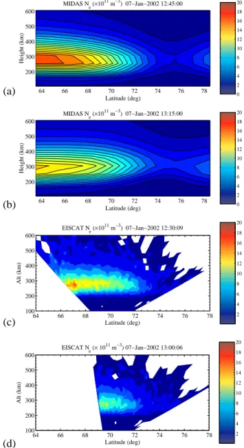
The MIDAS inversions result in one-hour movies of the three-dimensional distribution of electron concentration. These can either be shown as plots of electron concen-tration or maps of TEC (by vertical integration). In this case (Figs. 2a and b) we have chosen to plot a single two-dimensional slice of the electron concentration at the longi-tude closest to the EISCAT radar. As our MIDAS image grid was stepped in increments of 4◦longitude our slice actually encompasses the longitude range 18◦E–22◦E. The plots are restricted in latitude to the region encompassing the EISCAT radar scans, 64◦N–78◦N. The times of our images have been chosen to coincide with half-way through the EISCAT scan. Figure 2a shows the electron concentration at 12:45 UT and Fig. 2b at 13:15 UT. The peak electron density height is 280 km, and the main trough is clearly visible in both im-ages centred around 75◦N−76◦N. During this half-hour
pe-riod an overall decrease in the peak electron concentration is apparent. In Fig. 2a the electron density can be seen to range from 2×10¹¹m−2at 75.5◦N to 16×1011m−2at 67◦N. In Fig. 2b, the electron density at 75.5◦N is 3×10¹¹m−2, whilst that at 67◦N is 12×1011m−2.
Figures 2c and d show the distribution of electron concen-tration observed by the EISCAT radar for the scan starting
0 2 4 6 8 10 12 14 16 18 20 64 66 68 70 72 74 76 78 200 300 400 500 600 Latitude (deg) Height (km) MIDAS Ne (×1011 m−3) 07−Jan−2002 12:45:00 64 66 68 70 72 74 76 78 100 200 300 400 500 600 Alt (km) Latitude (deg) EISCAT N e (×10 11 m−3) 07−Jan−2002 12:30:09 2 4 6 8 10 12 14 16 18 20 0 2 4 6 8 10 12 14 16 18 20 64 66 68 70 72 74 76 78 200 300 400 500 600 Latitude (deg) Height (km) MIDAS N e (×10 11 m−3) 07−Jan−2002 13:15:00 64 66 68 70 72 74 76 78 100 200 300 400 500 600 Alt (km) Latitude (deg) EISCAT N e (× 10 11 m−3) 07−Jan−2002 13:00:06 2 4 6 8 10 12 14 16 18 20
(d)
(c)
(b)
(a)
Fig. 2. Electron concentration at the longitude of the EISCAT radar
between 12:30 and 13:30 UT: (a) and (b) plotted from GPS data using MIDAS; (c) and (d) plotted from EISCAT data.
at 12:31 UT and 13:00 UT respectively. In Fig. 2c, the peak electron density height is 275 km. At 75.5◦N, the electron
density is 2×10¹¹m−2, whilst at 67◦N it is 13×1011m−2.
The scan of Fig. 2d was halted prematurely due to a tem-porary problem with the radar. Comparing Fig. 2c back to Fig. 2a, good agreement can be seen between the two inde-pendent techniques.
Of particular interest is the overall agreement in absolute values of electron concentration. This can be partly attributed to the correct calibration of the radar observations using the dynasonde. The very small-scale structures (tens of km) ob-served in the radar scans would not be expected to be seen by the MIDAS imaging. The applicability of the vertical profile constraints used in MIDAS (from IRI95) are to be noted −
756 R. W. Meggs et al.: Simultaneous observations of the main trough 0 2 4 6 8 10 12 14 16 18 20 64 66 68 70 72 74 76 78 200 300 400 500 600 Latitude (deg) Height (km) MIDAS N e (×10 11 m−3) 07−Jan−2002 14:15:00 0 2 4 6 8 10 12 14 16 18 20 64 66 68 70 72 74 76 78 200 300 400 500 600 Latitude (deg) Height (km) MIDAS N e (×10 11 m−3) 07−Jan−2002 14:45:00 64 66 68 70 72 74 76 78 100 200 300 400 500 600 Alt (km) Latitude (deg) EISCAT N e (×10 11 m−3) 07−Jan−2002 13:59:46 2 4 6 8 10 12 14 16 18 20 64 66 68 70 72 74 76 78 100 200 300 400 500 600 Alt (km) Latitude (deg) EISCAT Ne (× 1011 m−3) 07−Jan−2002 14:30:06 2 4 6 8 10 12 14 16 18 20
(d)
(c)
(b)
(a)
Fig. 3. Electron concentration at the longitude of the EISCAT radar
between 14:00 and 15:00 UT: (a) and (b) plotted from GPS data using MIDAS; (c) and (d) plotted from EISCAT data.
the quiet ionospheric conditions have no doubt assisted in making this a suitable choice.
Figure 3a shows the electron concentration at 14:15 UT and Fig. 3b at 14:45 UT. The main trough is clearly visible in both images centred around 74.5◦N−75.5◦N. Between the two images there is an apparent southward movement of the trough, and this is confirmed by the EISCAT scans (Figs. 3c and d). Again it can be seen that the electron concentrations are decreasing over the half hour period between the two im-ages and they have decreased over the previous hour (com-paring back to Fig. 2).
In Fig. 3a the electron density can be seen to range from 2×10¹¹m−2at 75.5◦N to 9×10¹¹m−2at 67◦N. In Fig. 3b, the electron density at 75.5◦N is 3×10¹¹m−2, whilst that
0 10 20 30 40 50 60
Inversion TEC 07−Jan−2002 12:00:00 90 oW 0 o 90 o E 0o 10 oN 20 oN 30 oN 40 o N 50 oN 60 oN 70 o N 80oN 0 10 20 30 40 50 60
Inversion TEC 07−Jan−2002 13:00:00 90 oW 0 o 90 o E 0o 10 o N 20 o N 30 o N 40 o N 50 oN 60 oN 70 o N 80oN 0 10 20 30 40 50 60
Inversion TEC 07−Jan−2002 14:00:00 90 oW 0 o 90 o E 0 o 10oN 20 oN 30oN 40oN 50 oN 60 oN 70 o N 80oN 0 10 20 30 40 50 60
Inversion TEC 07−Jan−2002 15:00:00 90 oW 0 o 90 o E 0 o 10oN 20 o N 30oN 40oN 50 oN 60 oN 70 oN 80oN 0 10 20 30 40 50 60
Inversion TEC 07−Jan−2002 16:00:00 90 oW 0 o 90oE 0o 10 oN 20oN 30 oN 40 o N 50 oN 60 oN 70 o N 80oN 0 10 20 30 40 50 60
Inversion TEC 07−Jan−2002 17:00:00 90 oW 0 o 90oE 0o 10 o N 20oN 30 o N 40 o N 50 oN 60 oN 70 oN 80oN
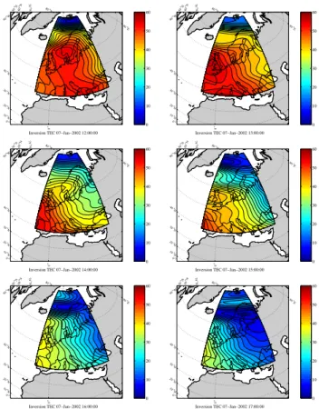
Fig. 4. Vertical TEC for each hour from 1200 to 1700 UT on 7
January 2002. Units are TEC units (1016electrons m−3)
at 67◦N is 7×10¹¹m−2. Comparing Fig. 3a with the EIS-CAT plot in Fig. 3c, it can be seen that the electron density at 75.5◦N, is 1×10¹¹m−2, whilst at 67◦N it is 7×10¹¹m−2. At 14:30 UT the EISCAT plot shows the electron density at 75.5◦N, is 1×10¹¹m−2, whilst at 67◦N it is 7×10¹¹m−2. However, these comparisons should be treated with caution, since the EISCAT images each represent a half-hour period, and the temporal and spatial variability is significant over this period.
Figure 4 shows the vertical TEC at each hour from 12:00 to 17:00 UT on 7 January 2002. The diurnal variation of the TEC in this sequence can be seen to follow that expected from the solar radiation. The main trough is clearly visible as the longitudinally distributed depletion of electron con-centration moving southwards from about 74◦N at 12:00 UT to about 65◦N at 17:00 UT.
4 Conclusions
Two entirely independent experimental techniques show si-multaneously the main trough over northern Scandinavia. The MIDAS images are taken from much larger spatial maps and demonstrate that dual-frequency GPS signals, moni-tored by a network of ground-based receivers, can be used to produce images of the main trough. These results are consistent with the expected behaviour of the main trough
during the early afternoon in the quiet, winter-time au-roral ionosphere. The EISCAT observations show very similarelectron concentrations, although they do not show the poleward wall of the trough. Hence it is difficult to be certain about the position of the trough minimum. However, the equatorward trough wall is well reproduced in both meth-ods, and the southward movement observed in the MIDAS images is confirmed by the EISCAT images.
MIDAS imaging using GPS has a very different role to play in ionospheric physics from that served by ISRs. MI-DAS can produce relatively low-resolution large area im-ages of the ionosphere at any time since around 1995 on-wards. This technique is of great interest for studying phys-ical events such as ionospheric storms and for obtaining an overview of large-scale gradients. MIDAS images are also a new and very useful source of information for improving ionospheric models. On the other hand, ISRs can show the details of the many physical processes occurring at smaller scales (several kilometres). The confidence that can now be put into the MIDAS images should allow the two techniques to be used together to investigate physical processes in the auroral regions across multiple scale sizes.
Acknowledgements. We are grateful to the International GPS Ser-vice for the use of GPS data, and we also acknowledge the use of the IRI model. RWM also thanks BAE SYSTEMS and the UK Engineering and Physical Sciences Research Council (EPSRC) for their support. EISCAT is an International Association supported by Finland (SA), France (CNRS), the Federal Republic of Ger-many (MPG), Japan (NIPR), Norway (NFR), Sweden (NFR) and the United Kingdom (PPARC).
Topical Editor M. Lester thanks two referees for their help in evaluating this paper.
References
Austen, J. R., Franke, S. J., and Liu, C. H.: Application of com-puterized tomography techniques to ionospheric research, Radio Beacon Contributions to the Study of Ionization and Dynamics of the Ionosphere and to Corrections to Geodesy and Technical Workshop, ed. A. Tauriainen, Ouluensis Universitas, Oulu, Fin-land, Beacon Satellite Symposium, 1986.
Austen, J. R., Franke, S. J., and Liu, C. H.: Ionospheric imaging using computerized tomography, Radio Sci., 23, 299–307, 1988. Beynon, W. J. G. and Williams, P. J. S.: Inchoherent scatter of radio waves from the ionosphere, Rep. Prog. Phys., 41, 910–956, 1978. Fremouw, E. J., Secan, J. A., and Howe, B. M.: Application of stochastic inverse theory to ionospheric tomography, Radio Sci., 27, 721–732, 1992.
Hargreaves, J. K.: The solar-terrestrial environment, ISBN0-521-42737-1, Cambridge University Press, 1992.
Mannucci, A. J., Wilson, B. D., Yuan, D. N., Ho, C. H., Lindqwis-ter, U. J., and Runge, T. F.: A global mapping technique for GPS-derived ionospheric total electron content measurements, Radio Sci., 33, 565–582, 1998
Mitchell, C. N., Kersley, L., and Pryse, S. E.: The effects of receiver location in two-station experimental ionospheric tomography, J. Atmos. S.-P., 59, 1411–1415, 1997.
Mitchell, C. N. and Spencer, P. S. J.: A three-dimensional time-dependent algorithm for ionospheric imaging using GPS, Ann. Geophys., 46, 687–696, 2003.
Na, H. and Lee, H.: Resolution analysis of tomographic reconstruc-tion of electron density profiles in the inosphere, Int. J. Inf. Syst. Technol., 2, 209–218, 1991.
Walker, I. K., Heaton, J. A. T., Kersley, L., Mitchell, C. N., Pryse, S. E., and Williams, M. J.: EISCAT verification in the develop-ment of ionospheric tomography, Ann. Geophys. 14, 1413–1421, 1996.
Rishbeth, H. and Williams, P. J. S.: The EISCAT ionospheric radar
−the system and its early results, Quart. J. Roy. Astron. Soc.,