Disambiguating words with self-organizing maps

(1)

Disambiguating Words with Self-Organizing Maps

by

Martin Marcel Couturier

Submitted to the Department of Electrical Engineering and Computer Science

in partial fulfillment of the requirements for the degree of

Master of Engineering in Computer Science and Engineering

MASSACHUSETTS INSTITUTE

at

the

OF TECHNOLOGY

MASSACHUSETTS INSTITUTE OF TECHNOLOGY

JUN

2 1 2011

June 2011

_LIBRARIES

©

_{Martin Marcel Couturier, MMXI. All rights reserved.}

_ARCHIVES

The author hereby grants to MIT permission to reproduce and distribute

publicly paper and electronic copies of this thesis document in whole or in

part.

Z14

Author ...

_//..

_V

_/K

_{.. r .}

_..

_{. ...}

...

D partment of lectxical Engineering and Computer Science

May 12, 2011

C ertified by

...

i ...

. .

.

., ... x - :

~...

...

Patrick H. Winston

Ford Professor of Artificial Intelligence and Computer Science

Thesis Supervisor

A ccepted by ...

...

Arthur C. Smith

Chairman, Department Committee on Graduate Theses

(2)

(3)

Disambiguating Words with Self-Organizing Maps

by

Martin Marcel Couturier

Submitted to the Department of Electrical Engineering and Computer Science on May 12, 2011, in partial fulfillment of the

requirements for the degree of

Master of Engineering in Computer Science and Engineering

Abstract

Today, powerful programs readily parse English text; understanding, however, is another matter. In this thesis, I take a step toward understanding by introducing CLARIFY, a program that disambiguates words. CLARIFY identifies patterns in observed word contexts, and uses these patterns to select the optimal word sense for any specific situation. CLARIFY learns successful patterns by manipulating an accelerated Self-Organizing Map to save these example contexts and then references them to perform further context based disambiguation within the language. Through this process and after training on 125 examples, CLARIFY can now decipher that shrimp in the sentence "The shrimp goes to the store. " is a small-person, not relying on a literal definition of each word as a separate element but looking at the sentence as a fluid solution of many elements, thereby making the inference crustacean absurd. CLARIFY is implemented in 1500 lines of Java.

Thesis Supervisor: Patrick H. Winston

(4)

(5)

Acknowledgments

Mom, Sam and M6mere for strong, independent and caring women. Together, you raised

me to be stubborn and fight for my dreams. Without your faith in me, I wouldn't have ever made it this far.

Patrick Winston for sticking with me the past four years and, in that time, imparting on me multitudes of both wisdom and knowledge.

Eric Timmons for always being there with great ideas and the patience to assist me whenever

I get stuck.

Erin Dostie for taking the time to stumble through my convoluted wording, helping me to more clearly present these ideas to others.

Ron, Alex and everyone else who has supported me along this journey. You have helped to make my MIT experience memorable and also played a part in molding who I am today.

(6)

(7)

List of Figures

2-1 A sample thread for the word mouse demonstrating how is-a relations can result in a distinct word sense. . . . . 23

2-2 Threads for mouse, cat and parrot combined into a classification tree of animal 24

2-3 two different word senses for the same word -mouse . . . . 25

2-4 sample thread bundle for mouse. These threads reflect the is-a relationships stored by W ORDNET . . . . 26 2-5 Internal representation of each of the two objects - mouse and cheese . . . . 27

2-6 Semantic Relation Modelling the Relation between Joe and laptop in Joe' s laptop. ... ... 27 2-7 A Semantic Net Modelling Relations Between Several Objects.. . . ... 27 2-8 mouse and cheese are the arguments in the event eat . . . . 28 2-9 "the mouse eats the cheese on a plate. " shown as a recursive event model. 29 2-10 Sample Trajectory: "The mouse f alls of f the desk" action: f all, object:

mouse, path: off the desk ... ... 29

2-11 Portion of a 2D grid SOM. The green is a newly inserted node . . . . 32

2-12 View of a dynamic SOM where new nodes can be easily added and connected to their neighbors. Red is the current node, green are its neighbors. . . . . . 32

3-1 Sample hill-climb of an SOM starting at green and ending at red. The values in each node are the distances of the node from the seed node. Note that the neighbors of all traversed nodes have also been examined. . . . . 37 3-2 Sample seed and current node trajectories... . . . ... 38

(12)

3-3 The two verb threads f all and go have a common junction at travel . . . 39

3-4 The subject threads mouse and prof essor have a common junction at organism. 39

3-5 The object threads desk and meeting have a common junction of entity . . 39 3-6 Thread Comparisons for Two Difference Objects... . . . . . . . 40

3-7 A successful hill-climb that eliminates the need to search a large portion of

the map... ... ... 42

3-8 A failed hill-climb, where the traversal ends at a local maximum. The true

maximum is highlighted with a distance of '5'. . . . . 43

3-9 An SOM enhanced with hub nodes (blue), providing accelerated jumps across regions of the m ap. . . . . 45

3-10 Initial random selection of hub nodes . . . . 47

3-11 A single iteration of shifting hubs apart by moving to further neighbors . . . 48

3-12 A possible ending hub configuration, after all hubs are pushed maximally apart 49

4-1 Sample Training Data Used by CLARIFY . . . . . . . . 54 4-2 Thread bundle for hawk . . . . 55

4-3 Thread bundle for cat . . . . 55

4-4 Thread bundle returned from WordNet to represent mouse (same as Figure 2-4) 56

5-1 Worst-case gradient traversal. All neighbors of traversed nodes are also ex-amined, implying in this case an

0(n)

traversal.. . . . . . . . . . 61 5-2 _{Average time of SOM look-ups given an SOM size for each look-up method .} ₆₂

(13)

List of Tables

2.1 Sample Distance Computation Between Nodes A and B with Weights(w): verb-50, subject-5, object-2... ... ... ... ... 31

3.1 3.2 3.3

3.4

3.5

Difference Object Between Trajectories in Figure 3-2...

Difference Object Between Current Node and Arbitrary Neighbor 1 Difference Object Between Current Node and Arbitrary Neighbor 2 Potential Difference Object Between Neighbor 1 and Seed Node example reward computation using a reward factor(f) of 0.85.

5.1 SOM performance results averages ordered by the size of the SOM for Standard(S)

a A. . . . . . . . . ...). . 62 Results for: Results for: Results for: Results for: Results for: Results for: Results for: Results for: Results for: Results for: "the "the "the "the "the "the "the "the "the "the

mouse climbs onto the tree" shrimp goes to the store." shrimp swims in the water." hawk flies to the oak." . ..

hawk runs to the finish line. jet flew to spain." . . . . . .

jet goes into the tank." glass goes in a window." glass falls to the floor." mouse fell off the desk"

5.2 5.3 5.4 5.5 5.6 5.7 5.8 5.9 5.10 5.11 . . . . 6 4 . . . . 6 4 . . . . 6 4 . . . . 6 5 "1 . . . . 65 . . . . 6 5 . . . . 6 6 . . . . 6 6 . . . . 6 6 . . . . 6 7

and Accelerated(A) look-ups.

(14)

(15)

Chapter 1 Introduction

e In this section you will learn how CLARIFY aids in the attempts to understand language, and in particular the element of language targeted. " By the end of this section, you will understand why CLARIFY is

important. You will also know which parts of this thesis to read for a more detailed discussion.

1.1 Big Picture: Representations Require an

Understand-ing of the Subjects

Words have power because they represent an underlying concept. A word is not a concept

by itself, but a handle on an underlying model. It allows the concept to be easily packaged,

used and modified. Patrick Winston notes "names give us power. " Words allow humans to share information by passing around finite pieces of meaning.

Consider the word mouse, as in "the mouse ran from the cat. " In this sentence, mouse is given the meaning of an animal, a rodent that is known for its cheese-loving personality. Hearing the word mouse in this context gives you an image of the literal translation of mouse and not the word used to refer to it.

(16)

It is interesting that this sense of a rodent is not exclusive to the handle. In your experiences, you may have tied the concept of a small gray rodent to other handles such as shrew or even rodent. Hearing any of these handles may have the effect of triggering the same imagery, depending on the level of specificity warranted through your own language and informa-tion processing. Other languages use different handles to link to a similar internal sense. You would hear a Frenchman refer to a mouse as une souris or a Spaniard refer to it as un rat6n. Each of these is just a different handle that leads to a sense of a little gray rodent.

It is also possible for one handle to refer to more than one concept. Consider another sentence, "the mouse clicks on the folder." This time mouse represents an electronic object used for pointing, clicking and selecting. Additionally, mouse can refer to different word-senses sentences such as in "that punch left a mouse under your eye" or "the

mouse ran from the fight."

Despite the fact that sentences possess different senses for mouse, as a fluent English speaker, you are able to infer the correct representation to use for mouse. This occurs because you have previously tied the handle of mouse to that representation and are able to retrieve information on the concept and not the word itself. Homonyms, such as mouse are very common in the English language, and yet somehow English speakers are able to extract the correct meaning for mouse, based on the context of the sentence.

In some cases, the correct meaning of a word may be unclear, such as in "the mouse f ell

of f of the desk. " Is this referring to a computer mouse, a rodent, or maybe a shy

com-puter nerd who was screwing in a light bulb? Disambiguation of this phrase would require reading deeper into the context of the sentence.

Addressing the problem of language comprehension requires a model of the human word disambiguation process. If a computer is to learn to understand language, as humans do, it

(17)

needs some way of building this model. If a computer is to model word disambiguation, it must first understand the subtleties behind the words. Understanding words, however, first requires understanding the different connotations of a single word.

In developing this model, there are several issues that must be accounted for; how are various word-senses obtained, how are the examples that tie a word-sense to a particular context stored, and how can a computer be programmed to make rapid use of these learned examples to disambiguate new word-senses? GENESIS, described in detail in Chapter 2, is a system that has machinery for satisfying each of these questions. The machinery is capable of pars-ing English stories and performpars-ing higher level story comprehension. The parspars-ing process requires that GENESIS already possess mechanisms for identifying and storing word-senses.

I discuss some specifics of this machinery in Section 2.1.

1.2 CLARIFY

Chooses One Relevant Meaning

When reading a story, GENESIS first parses the input, identifying both syntactic information about the input as well as the words individually. Each of the words processed is queried to WORDNET [Miller, 2006], which provides hierarchical classifications of words, such as a mouse is a type of rodent which is a type of animal. These hierarchies allow the system to generate concrete representations for each of the words. I further discuss WORDNET in

Section 2.2.3

What happens when a homonym is passed into WORDNET? It sends back information for all the different meanings of that word. WORDNET has no way of knowing which meaning is intended by GENESIS and therefore returns all of them.

(18)

1.2.1 Keeping All Meanings Leads to Learning Errors

One solution to receiving all of these words is to save all meanings of the word and not force the system to decide upon any one. This would give the system some arbitrary grasp on a word. Unfortunately, this approach risks comprehension errors. For example, imagine de-scribing a computer mouse to a computer, while the computer is storing the learned qualities about a generic mouse. It does not matter what kind of mouse the computer thinks this is, because when later prompted for information about mouse, the computer can return all the information it was given. The error in its representation is masked from the user by the duplicity of the abstraction mouse.

A visible problem arises, however, when the user switches to discussing a living mouse.

The computer still assumes the generic term mouse, and so it starts returning information about computer mice. Because of this overlap, it becomes vital that the two different types of mice are two different objects and their meanings are kept disjoint. In order for a com-puter to learn correct information about one type of mouse, it needs to be able to identify which mouse is being discussed. CLARIFY enhances the GENESIS system by deciding upon one word-sense over another in ambiguous situations.

1.2.2 GENESIS Selected the First Definition and Used it

Currently, GENESIS attempts to sidestep the problem of incorrect word-sense choice. It stores all meanings returned by WORDNET in a word bundle, and references it with the first thread in that bundle. As I discussed, this can result in problems when the meaning of a word changes. GENESIS is fortunate that the first meaning returned by WORDNET is the most probable meaning for the word, meaning that GENESIS is right, most of the time.

(19)

1.2.3 CLARIFY's

Decisions Reflect its Experiences

Instead of selecting the first meaning of a word as the default meaning, CLARIFY attempts to deduce the word meaning from sentences it has already observed. For example, seeing the sentence "the mouse fell off of the desk" would cause CLARIFY to look at other sentences that contain concepts of falling off of furniture. It would then choose the meaning of mouse that best matches with its learned pattern for falling off furniture.

This raises an interesting situation of human imitation. Sometimes, humans are capable of wrongly disambiguating words. For example, a computer scientist who spends all day at his computer would more likely interpret "the mouse f ell of f of the desk" as a computer mouse than a chef would. This is merely due to the experiences and associated connotations

each finds himself in.

CLARIFY is no different in this respect. Its decisions are heavily dependent on the things

that it has previously encountered. If it has previously learned a lot about animals climbing and falling off of things, the algorithm would likely find that a mouse that falls off of a desk is a rodent. On the other hand, if the system has read many examples of different electronic objects being dropped, placed or moved, it would likely consider a mouse to be a computer mouse.

1.3 Self-Organizing Maps Look-up the Best Word for a

Context

The goal of CLARIFY is to locate a relevant example in memory that closely matches the sentence under question. In this way it can decide which word sense is the best fit for the sentence. Using memory raises the issue of how to best store and lookup examples. The current memory system employed by GENESIS is made up of several Self-Organizing Maps (SOMs) [Kohonen, 2001]. These maps are effective for storing sentence structures, but their

(20)

complexity prevents them from being efficient at making the needed lookups.

1.3.1 An Accelerated SOM Allows CLARIFY to Perform More

Effi-ciently

CLARIFY _{has two phases, a training phase and a disambiguation phase. In the}

disambigua-tion phase, it is expected that the selected memory system will be able to quickly determine the most likely connotation for the provided word. SOMs are a good choice for this task, but due to slow retrieval times, the mechanism grows clunky as it learns more examples. Fortunately, the data within an SOM is naturally clustered. Clusters make it feasible to hill-climb through the map, following a gradient of likeliness to the target example. Using gradient traversal isolates the target more rapidly than the traditional method of lookup.

1.4 What is Next?

"

Relevant Technology discusses the machinery that uses WORDNET to create repre-sentational word-senses using threads. It also discusses the Self-Organizing Maps that make up the primary model of CLARIFY's memory system.

* SOM Acceleration describes the algorithm used to modify SOMs in order to speed

up the lookup process.

" Word Disambiguation walks through the process by which CLARIFY disambiguates word-senses using its training examples.

" Results discusses the effectiveness the disambiguation process.

(21)

Chapter 2 Relevant Technologies

" In this section you will gain a basic understanding of the various tech-nologies used by GENESIS to model stories. These technologies include

threads, WORDNET, and event models.

" By the end of this section, you will understand how these technologies can be integrated with a Self-Organizing Map memory system, to later be used for word disambiguation by CLARIFY.

2.1 GENESIS

The GENESIS system is an ongoing research project of MIT's GENESIS group. The mission

of the project is to interpret stories written in common English. For this purpose, GENESIS

must first parse the English sentences and build internal representations. It is this initial parsing which CLARIFY assists.

Once the representations are constructed, the system looks for places where it can apply common sense knowledge, drawing contextual conclusions from the story. An example of a common sense rule is that murder results in death. If GENESIS reads "Macduf f kills Macbeth, " it can apply this murder rule to conclude that "Macbeth is dead. "

(22)

appara-tus to isolate higher level plot units such as revenge, successes or pyrrhic victory [Nackoul,

2009]. It locates the plot units by looking for patterns of events characteristic to each. For

example, to identify an instance of revenge, GENESIS looks for the pattern

[("xx

harms yy") causing ("yy harms xx")]. After GENESIS has applied all common sense rules and isolated all plot units, it outputs a "Reflection Analysis" describing each of the plot units identified.

2.1.1 GENESIS is Modular

GENESIS is easily expanded. It makes use of a propagation architecture allowing different components to communicate through the use of a wire paradigm [Winston, 2008]. These "wires" connect various components with one component publishing information on one end, and a subscribed component "listening" on the other end. Within this architecture it is therefore easy to add or remove components to the system by merely connecting a few wires.

In order to connect CLARIFY to the GENESIS system, CLARIFY listens to trajectories (2.3.3) and broadcasts disambiguated threads (2.2). If CLARIFY is un-wired from the system,

GEN-ESIS continues to perform without any problems.

2.2 Threads Store Word-Sense

Individual words can be related via a hierarchy of specificity. For example, a mouse is a type of rodent, which is a type of mammal, which is a type of animal, etc. Note the use of the phrase is-a. This phrase defines a word in terms of something more general than itself within certain specificities inherent to that individual context. If you recurse, climbing up several is-a relations, you will eventually reach some root of generalization, such as thing or action. The resulting path of is-a relations, from the word to the root, is called a thread as defined by researchers of the MIT Al Lab [Vaina and Greenblatt, 1979]. Threads can serve as a representational word-sense of a word, defining any situation in a given context

(23)

and through a specific set of understood patterns previously discovered and learned by the program.

Figure 2-1 - A sample thread for

result in a distinct word sense.

the word mouse demonstrating how is-a relations can

2.2.1 Threads are Easily Comparable

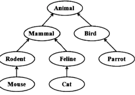
Because words higher up the thread are more general than the word itself, it is often the case that these ancestors are also part of other threads. For example, a mouse is a descendant of animal, but so is a cat or a parrot. With these thread commonalities, it is possible to superimpose different threads obtaining a classification tree. When comparing multiple threads, the two threads with the lowest common ancestors are said to be most alike. In Figure 2-2, you can see the threads for mouse, cat, and parrot superimposed into a hierar-chy. While mouse and cat have a common ancestor of mammal, mouse and parrot only join at animal. With this example it is clear that mouse and cat are more closely related, due to their lower ancestral root.

Using this intuition, it is possible to devise a way of computing how different two threads are. To compute the distance, we add up how much work it is to get from one word to another through their threads. A simplified approach counts the steps in the joined tree along the ..... ... .... ... .. . ....

(24)

Figure 2-2 - Threads for mouse, cat and parrot combined into a classification tree of

animal

shortest path between nodes. If using this approach, the distance between between mouse and cat in 2-2 is four.

Because ancestors higher in a tree have exponentially more descendants, climbing higher up the tree should incur exponentially higher cost. The metric used for this thesis follows a base two incrementing approach starting at power 0. When examining the mouse thread, to go from mouse to animal, the tree must be climbed three steps and therefore the cost of climbing to animal is 23-1 = 4. This is computed for both threads up to the common ancestor and the scores added together. To complete this example, the new distance between mouse and cat is four, while the distance between mouse and bird is five.

Note that for threads with 0 steps to common junction, the score is 2-1 = _2', which is clearly wrong. I account for this by always taking the floor of the distance, defining the distance between two identical threads as 0 rather than I without disturbing any of the₂ other distance scores.

2.2.2 Threads Make Multiple Word Senses Possible

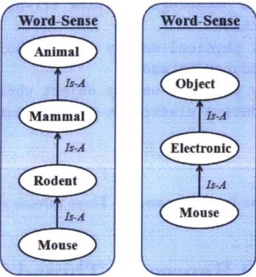
When a word is observed, it is possible that it can take on one of several meanings. The word mouse can imply either a rodent mouse or a computer mouse. Threads support this

(25)

quality of multiple word senses because each word sense is characterized by a unique thread. In Figure 2-3, you can see that two threads for mouse are different, even though the word at the bottom is the same.

Word-Slense

Word-Sgnse

Animal

hsA _Object Mammal ' -A Electronic

Rodent

hei-Is-A

Mouse

Figure 2-3 - two different word senses for the same word -mouse

2.2.3 WORDNET Enables Thread Construction

The GENESIS system obtains thread information by making queries to the WORDNET database. The database stores various word relationships -homonyms, antonyms, synonyms, hyponyms and hypernyms. The hyponym relationship is particularly useful because it stores the is-a relationships discussed earlier. When GENESIS queries the database it is able to ob-tain the complete hyponym information for the queried word and use it to construct a thread.

When words have multiple word senses, WORDNET returns hyponym information for each of the various word senses. GENESIS processes the information to create each of the threads and stores them in a thread bundle.

(26)

---<bundle>

<thread>thing entity physical-entity object whole living-thing organism animal chordate vertebrate mammal placental rodent mouse</thread>

<thread>thing entity abstraction attribute state condition

physical-condition pathological-state ill-health injury bruise shiner mouse</thread>

<thread>thing entity physical-entity object whole living-thing organism person mouse</thread>

<thread>thing entity physical-entity object whole artifact instrumentality device electronic-device mouse</thread> </bundle>

Figure 2-4 - sample thread bundle for mouse. These threads reflect the is-a relationships

stored by WORDNET

2.3 Event Models Represent Thread Relations

Threads are useful for representing word-senses. They are not however capable of capturing deeper concepts that exist in phrases and sentences. For example, a thread cannot model the event between mouse and cheese in "the mouse eats the cheese. " To handle concepts like this, GENESIS implements a frame architecture similar to those defined by Minsky [1974], to wrap concepts of varying complexity in higher abstracted concepts.

2.3.1 Semantic Nets Frame Threads

Threads are at the base of frame abstractions and are used as building blocks in the con-struction of higher level more sophisticated concepts.

(27)

mouse

183 cheese

188

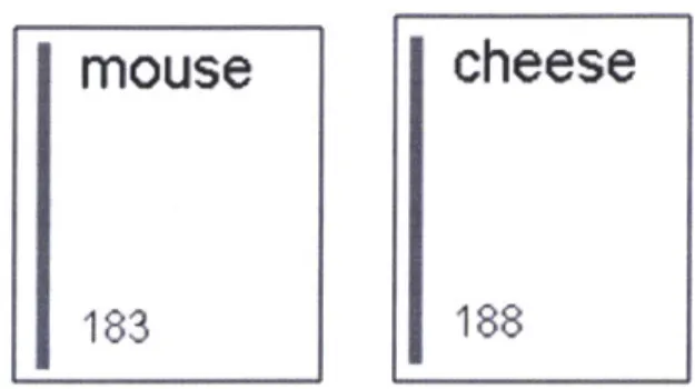
Figure 2-5 - Internal representation of each of the two objects -mouse and cheese

Directly above thread objects are semantic relations. A semantic relation models the cor-relation between multiple objects. This results in a greater understanding of each object in the relation.

Figure 2-6 - Semantic Relation Modelling the Relation between Joe and laptop in Joe' s laptop.

Using simple semantic relations, GENESIS is able to compile a semantic net, modelling the various relations between many objects.

A Semantic Net Modelling Relations Between Several Objects

(28)

2.3.2 Event Models Also Frame Semantic Relations

On top of the semantic net layer, GENESIS frames together concepts that have been modelled

by semantic relations. This layer relates concepts by the events that can occur between them.

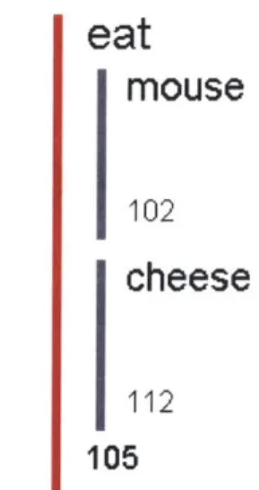
An event consists of a verb that often takes an array of concepts as arguments. For example in Figure 2-8, the verb eats relates mouse and cheese, a subject and a direct object. The verb is depicted spanning both of its arguments. In this case, the concepts are both threads, the simplest form of a semantic relation, but the event eat would handle, in the same fashion, the relation Joe' s mouse as a subject.

eat

mouse

102

cheese

112

105

Figure 2-8 - mouse and cheese are the arguments in the event eat

Because both event models and semantic nets take concepts as their arguments, and concepts have varying levels of complexity, the result can be a complicated arrangement of events and relations used to model an overall concept. This result is also a concept, and so you can imagine an unbound recursive model of nested concepts. Figure 2-9 shows the model for "the mouse eats the cheese on a plate."

(29)

on

eat

Imouse

284

I

cheese

286

285 I

plate

289

288

Figure 2-9 - "the mouse eats the cheese on a plate." shown as a recursive event

model.

2.3.3 This Thesis Handles Only Trajectory Events

Through the use of semantic relations and events, GENESIs is capable of modeling many different structures. The most complicated of these is a trajectory, which involves some object, moving along some path. An example trajectory is shown in Figure 2-10. I restrict

fall

I

mouse

209

path

off

I

at

Sdesk 234 235

231

232

Figure 2-10 - Sample Trajectory: "The mouse falls of f the desk" action: fall,

ob-ject: mouse, path: off the desk

my scope to deal only with examples of trajectories for two reasons. First, trajectories ...

(30)

are complex enough to provide an adequate representation of all other semantic structures. Second, the solution I propose for word disambiguation would require a different memory system for each semantic structure. As a result, handling different structures does not enhance the proof of concept for my proposed memory system. The system I propose learns from observed trajectories, in order to make informed word-sense disambiguation of words in future trajectories.

2.4 SOM's Store and Cluster Observed Objects by

Sim-ilarity

In order to learn from observed trajectories there needs to be a memory system capable of storing the trajectories in a useful fashion. SOMs satisfy this requirement by simplifying the process of saving and organizing observed trajectories.

2.4.1 Nodes Implement Distance Metrics

SOMs work by converting objects into nodes and placing them into a map. Nodes implement a distance metric through which various nodes are compared. Nodes with smaller distances between them are considered to be more alike than nodes with larger distances. As a result, it is possible to use this distance metric to organize the SOM such that similar nodes are clustered close to each other, by connecting them as neighbors.

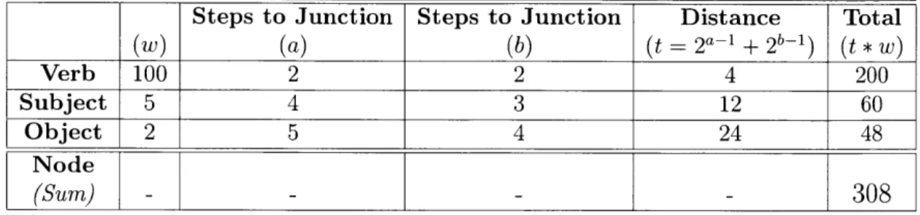
The metric for computing node distances depends on the contents of the SOM. Because the SOM used by CLARIFY stores trajectory objects, which are composed of threads, I elected to make use of the distance properties of threads discussed in 2.2.1. You can think of a trajectory as being composed of three main parts -the verb, the subject, and the path object. To compute the distance between two trajectories, you compute the distance be-tween each of the thread pairs: verb/verb, subject/subject, path/path and add them together. Whereas the subject and path are arguments of the verb, the verb is considered the most

(31)

critical aspect of the trajectory, and thus holds a larger weight than the other two thread pairs.

Table 2.1 - Sample Distance Computation Between Nodes A and B with Weights(w):

verb-50, subject-5, object-2

Steps to Junction Steps to Junction Distance Total

(w) (a) (b) (t = 2a1 2 1) (t*W) Verb 100 2 2 4 200 Subject 5 4 3 12 60 Object 2 5 4 24 48

Node

(Sum) - - - - 308

2.4.2 Inserting Looks for Most Similar Neighbors

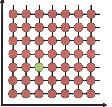
When a new node is to be inserted in the SOM, it must first be compared to every other node in the map, looking for the nodes with the most similarity. There are two SOM styles that implement this task in different ways. One SOM implements a two dimensional grid to store nodes (Fig. 2-11). A new 'seed' node is inserted at the point in the grid where the currently residing node has the smallest distance from the seed. All of the nodes surrounding that location are assigned as the seed's neighbors and are modified slightly, causing them to more closely resemble the seed. The downside of this approach is that the system is restricted to a static SOM with finite size. It replaces existing nodes with new nodes. As a result, I chose not to implement this type of SOM for CLARIFY.

The alternative is to create a dynamic SOM that has no fixed size. Each node is inserted in an arbitrary location but remains linked to the nodes with the smallest node distance, thus becoming its neighbors (Fig. 2-12). This is done by iterating through all the nodes in the map, keeping track of the n nodes with the smallest distance from itself. The variable n is the maximum number of allowed neighbors and has a predefined value. After iterating through the entire map, two-way neighbor links are established thereby creating a network of interconnected nodes. n limits the branching factor of my hill-climbing search (3.2.1).

(32)

Portion of a 2D grid SOM. The green

Figure 2-12 - View of a dynamic SOM where new nodes can be easily added and connected

to their neighbors. Red is the current node, green are its neighbors. ...

AdIk

AdIk

Ak

v Mv 14

(33)

In both SOM's, inserts occur in O(n) time, where n is the current size of the map. For the first SOM, n is a large constant, whereas in the second case, n starts small, but increases on every insert.

Note - though CLARIFY uses a dynamically resizing SOM, points regarding SOMs will be depicted using a 2D grid in future sections. This is done for the benefit of the reader, because it makes neighbors, paths and clusters clearer.

2.4.3 Lookup Takes as Long as Insert

When a node is looked up in the SOM, a very similar procedure to insertion is followed. The

SOM searches through all of its nodes looking for a node that most closely resembles the

seed. After looking through the entire map computing distances between the target node and each of the existing nodes, the SOM returns the single node with the shortest overall node distance. This procedure is the same in both versions of an SOM mentioned in the above section. Because the entire map must be examined, the SOM retrieval time runs in

O(n) time, similar to inserts.

In some instances, an O(n) lookup time is acceptable. Consider however a case where the map is very large and the system seeks to use the SOM for some computation that requires a large number of lookups. The result is a very long processing time. In the next chapter, I propose a modification to an SOM to speed up the lookup time, allowing a trained SOM to be used to aid in the task of word disambiguation.

(34)

(35)

Chapter 3 SOM Acceleration

e In this section you will learn about the clustered nature of SOM's and how this feature can be manipulated in several ways to speed up look-ups in dynamically resizing SOM's.

* By the end of this section, you will know enough about the acceleration mechanism to implement your own SOM look-up.

3.1 Disambiguation Preview

Imagine a situation where you have a collection of trajectories. Among those trajectories are some demonstrating falling actions, others demonstrating swimming actions, etc. At some point you receive a new trajectory that describes a leaf falling from a tree. You know that a leaf can be one of several things: a part of a plant, a part of a table, or a piece of paper. In your uncertainty, you decide to compare this trajectory to your overall collection of trajectories, hoping to find some clue of what definition is the best fit. The comparison strategy involves looking for a trajectory that looks most like your new trajectory.

As you begin to examine the collection, you are unsure of how to search for the trajec-tory that is the best match. In a naive approach, you could search through every single trajectory in the collection, but you realize that your collection is huge and you instead

(36)

decide to find a speedier way of locating the trajectory. One way involves manipulating the nature of your collection, thereby only searching relatable trajectories in the map.

3.2 SOMs Facilitate Nodal Gradients

By design, neighbors of any node in an SOM share some similarity to the node. As a result,

if one node is a neighbor to two other nodes, there is a high chance that the other two nodes also share similarities. If they share enough similarities, then there is a good chance that they also are neighbors. This organization usually results in clustered groups of similar nodes in various positions around the map. Nodes that lay outside other clusters are different from those clusters and are often an intermediary on a path between clusters. These intermediary nodes also have neighbors that are in some way similar to themselves. As a result the node clusters can be considered to be connected by a gradient path, where the gradient captures how neighbors are similar.

3.2.1 Difference Network Between Nodes Allows for Faster

Gradi-ent Traversal

The gradient layout of the nodes of an SOM makes several search methods reasonable. The first of these methods is hill-climbing. When looking for the most similar node in the map to a specific seed, hill-climbing would begin by selecting an arbitrary node. This node would be compared to the seed node and a score computed. Next the program would examine each of the neighbors of the current node, computing distance scores with the seed node. If a neighbor has a smaller distance, hill-climbing would advance to the location of that neighbor and continue the search, forever ignoring the other neighbors of the previous node. In cases where multiple neighbors have a smaller distance to the seed node than does the current node, the neighbor with the smallest distance is selected. Hill-climbing follows a heuristic to always select a node with the most matching improvement.

(37)

12 -

10

8

-'20 1815

Figure 3-1 - Sample hill-climb of an SOM starting at green and ending at red. The values in each node are the distances of the node from the seed node. Note that the neighbors of all traversed nodes have also been examined.

There are two downsides to hill-climbing. The first, local maxima, is discussed in Section

3.2.3. The second downside is the way in that hill-climbing heuristics are evaluated. For

an SOM that handles trajectories, every time a node is traversed, the distance between the seed and each of the node's neighbors must be computed. The distance computation as described in Section 2.4.1 runs in linear time to the size of the trajectories. This is because each thread pair must be iterated over in order to find the common junction. Only after the common junction has been found can the distance between nodes be computed. That final computation occurs in constant time.

.

(38)

Because SOM look-ups occur during the runtime of CLARIFY's testing phase (Section 4.1.2), some time can be saved by moving a portion of this computation to training time. To ac-complish this, I implement the concept of a Difference Network as described by Winston

[1970]. This network examines each neighbor pair, creating a difference object containing

thread junctions for each of the thread pairs in the nodes. Additionally, the object contains the indexes of those junctions for each of the threads as well as the total thread lengths. All of the difference objects are constructed before look-ups take place. With these difference objects, look-ups no longer need to compute distances between nodes, but instead compute changes in the distances by comparing the differences.

Difference Network traversal still follows a hill-climbing algorithm. When a seed is passed to the SOM for look up, a difference object is created between the seed and the current node, which is then used to represent the overall distance between the seed and current reference node. When deciding where next to move along the gradient, each of the difference objects with the current node's neighbors is compared to the difference object of the current node and the seed. By comparing the common junctions and their indexes, it is possible to tell if one of the neighbors is more or less similar to the seed node compared to the initial node.

Consider the nodes containing these trajectories:

Seed: the mouse fell off the desk

Current Node: the professor goes to the meeting

Figure 3-2 - Sample seed and current node trajectories

Looking at the verbs for each of these trajectories, we can see that the threads possess a common junction of travel at a zero-based index of one.

(39)

<thread>action trajectory travel fall</thread> <thread>action trajectory travel go</thread>

Figure 3-3 - The two verb threads f all and go have a common junction at travel

Looking next at the subjects of the trajectory, the threads have a common junction of organism at index six.

<thread>thing entity physical-entity object whole

living-thing organism animal chordate vertebrate mammal placental rodent mouse</thread>

<thread>thing entity physical-entity object whole living thing organism person adult professional educator

academician professor</thread>

Figure 3-4 - The subject threads mouse and professor have a common junction at organism.

Lastly, the place objects for these two trajectories have a common junction of entity at index two.

<thread>thing entity physical-entity object whole artifact instrumentality furnishing furniture table desk</thread> <thread>thing entity abstraction group social-group gathering meeting</thread>

Figure 3-5 - The object threads desk and meeting have a common junction of entity

Let us compress this information to a difference object, in a form that is easier to use: Table 3.1 - Difference Object Between Trajectories in Figure 3-2

Junction Index Length of Current Length of Seed

Verb travel 1 4 4

Subject organism 6 13 14

(40)

Now imagine two other difference objects that exist between the current node and two of its neighbors:

Table 3.2 - Difference Object Between Current Node and Arbitrary Neighbor 1

Junction travel person abstraction Index 1

7

6

Length of Current Length of Neighbor 1

4 4

13 10

7

9

Table 3.3 - Difference Object Between Current Node and Arbitrary Neighbor 2

Junction Index Length of Current Length of Neighbor 2

Verb go 2 4 3

Subject adult 8 13 9

Place gathering 5 7 15

When comparing two difference objects comparing alb and ajc, the junction occurring higher in the tree, or with the lower index is the junction that is carried over to the difference object between blc. For example, if you have differences between the following pairs of threads:

1. <thread>action trajectory travel fall</thread>

2. <thread>action trajectory travel go</thread> and:

<thread>action trajectory travel fall</thread>

<thread>action trajectory travel fall fall-into</thread> Figure 3-6 - Thread Comparisons for Two Difference Objects

(1) and (3) are the same thread, so the cornmon junction between (2) and (4) is travel,

which is the higher junction of the two differences. Using this principle, it is possible to quickly predict the difference objects between the seed and each of the neighbors.

If the common junctions in two difference objects are the same, it is possible that the

com-mon junction in the new difference object is further down the tree. dog and cat both differ

Verb Subject

(41)

from bird at animal, but between themselves they have a common junction at mammal. In cases such as these, the new common junction is found by starting at the current junction and stepping down the threads until they differ.

Table 3.4 - Potential Difference Object Between Neighbor 1 and Seed Node

Junction Index Length of Neighbor 1 Length of Seed

Verb travel 3 4 4

Subject organism 6 10 14

Place entity 5 9 11

Choosing which neighbor to go to, is a matter of comparing length of the threads along with the indexes of the common junctions. These values can be used to quickly compute the overall distance and test if the distance of a neighbor is less than the distance of the current node, thereby resulting in constant speed-up of the hill-climbing algorithm.

3.2.2 Gradient Traversal Eliminates Extraneous Searching

The primary motivation for using an algorithm that uses a gradient traversal search is to avoid searching many unnecessary nodes. If the distance between some node and the seed node is five, it would make no sense to move to a node whose distance from the seed is ten. Recall that traditional SOM look-ups search an entire map. For each node in the map, the distance between the node and the seed is computed and the node with the smallest distance is saved. By using a gradient approach instead, I make the assumption that the clustering of the map is well formed. Once a gradient is followed to the top of a peak where none of the neighbors possess a smaller distance, it does not make sense to climb back down the peak looking for other nodes. Hill-climb searches make it possible to locate the best match for a seed, while often searching only a small fraction of the map.

(42)

20

18

15

Figure 3-7 - A successful hill-climb that eliminates the need to search a large portion of

the map.

3.2.3 Gradient Traversal has Local Maxima

As with other hill-climbing applications, it is possible that the clustered nodes in the SOM contain local maxima. As a result, hill-climbing can get stuck at a local maxima mistaking it for the best match for a seed when there are better options elsewhere (Fig. 3-8).

In order to protect against local maxima, the hill-climbing algorithm I implement uses mul-tiple random samplings. There is a predefined number of searches to be performed on the map for a single seed. For each search a starting node is chosen at random, and the gradient

(43)

1 I

I

Figure 3-8 - A failed hill-climb, where the traversal ends at maximum is highlighted with a distance of '5'.

a local maximum. The true

traversal is executed until some maxima is reached. The algorithm is then repeated several times with different starting nodes, each time looking for a new local maxima. The best of the local maxima is then returned as the overall maxima. Unfortunately, re-sampling is a trade-off between accuracy and efficiency, and thus the number of re-samplings must be adjusted through experimental trials.

Though multi-sampling costs more time than a single gradient traversal, it can be guaranteed to take at most as long as a traversal of the entire map. Hill-climbing has a deterministic quality. If a node is ever examined in a search through the map, the path out of that node

(44)

will be the same for each subsequent search. Because of this, if a node has already been traversed it can be flagged to prevent re-entry. Additionally, a neighbor is examined but not selected it is not part of an ideal, and therefore all examined neighbors are flagged as well.

If all nodes have been examined, each will be flagged and thus the search will be forced to

quit, having not searched more than in the traditional SOM look-up.

3.3 Highways Speed up Difference Network

Another enhancement I introduce for SOM look-ups is the concept of hub nodes. Hub nodes follow with the metaphor of airline hubs. Imagine traversing the country, driving from one city to the next. In some cases, such as traveling between Boston and Plymouth, it is best to remain in a car and drive. In other cases, such as traveling between Boston and Palo Alto, it is significantly faster to first drive to Logan Airport, a hub, and fly to SFO, another hub, before resuming local travel by car. This back-gate 'hub traversal' bypasses a large chunk of time that would have been spent traveling across country in an automobile.

In my SOM, I follow this pattern, designating certain nodes as 'hub' nodes and allowing a single step traversal between any two hub nodes (Fig. 3-9). This implies that if, during a look-up, the gradient traversal lands on a hub node, it can proceed to either that node's regular neighbors, or any of the other hub nodes.

(45)

Figure 3-9 An SOM enhanced with hub nodes (blue), providing accelerated jumps across

Figure 3-9 - An SOM enhanced with hub nodes (blue), providing accelerated

jumps

across regions of the map.

3.3.1 How to Select Key Nodes

Hub nodes can be selected according to various metrics. Each metric possesses its own pros and cons. For example, one metric would choose to connect nodes that are most different. This approach would provide the largest speed up for samplings that initiate very far from their target nodes. However, this method is not easily adapted to handle multiple nodes. Because the nodes are so different, it is possible that the hubs are located on sparsely con-nected regions of the map, implying that the gradient traversal may never find them. . ... . ... ... ... -... . .. ...

(46)

An alternate metric selects the nodes with the most neighbors. Because these nodes have the most neighbors, there is a higher probability that the traversal of the difference network would arrive at the hubs. Unfortunately, due to the clustering in SOMs, it is common for the nodes possessing the most neighbors to also be neighbors to each other. This would require an additional metric that checks to make sure all hubs are some specified number of steps apart. Having two neighbors both be hubs reintroduces search complexity to the graph, without providing any significant benefits. Additionally, with any SOM, it is common for many nodes to all have the maximum number of neighbors, and so it would likely result in many hubs.

The metric I chose to implement for CLARIFY seeks to find a specified number of hub nodes evenly spaced around the map. The number of hub nodes I use is equal to the square root of the size of the SOM. Because the hub nodes are fully connected, it is ideal to have just enough hubs to represent the map. Having too many hubs, however, could result in a

(47)

To initialize the hub nodes, I implemented an algorithm that begins by randomly selecting the specified number of hub nodes in the map.

Figure 3-10 - Initial random selection of hub nodes . .... ... ...... .... ... ...

(48)

Each hub is then compared to each of the other hubs, using a Breadth-First Search to ex-amine the shortest path between them. If a hub possesses a neighbor that is not part of a shortest path to another hub, that neighbor takes its place as a hub, thus extending the shortest paths between hubs.

it

Figure 3-11 - A single iteration of shifting hubs apart by moving to further neighbors

(49)

-This algorithm is looped over until no hub can be pushed further out. At this point the hubs are considered to be well dispersed.

I

AIl

I\&w

Figure 3-12 - A possible ending hub configuration, after all hubs are pushed maximally

apart

Once all hub locations have been fixed, another stage of hub processing occurs. In this stage, every node in the SOM performs a Breadth-First Search looking for the nearest hub. The distance to that hub is stored and is later used for an alternate gradient traversal, described in the next section.

(50)

3.3.2 Markov Rewards Encourage the Use of Hub Navigation

One risk of the hub enhancement is that traversal may never reach the hub nodes at all. This would be unfortunate if the hubs actually provide access to the true maxima and the gradient traversal is caught up in local maxima. A partial solution to this problem was inspired by Markov Transition Reward Models [Russel and Norvig, 2010]. Following with these models, I introduce incentive to the gradient traversal, encouraging it to access the hub network. In addition to looking for the most similar node to a seed node, the look-up process now has a back-off option that compares the seed to the hub nodes.

At the start of an SOM look-up, the system begins by first comparing the seed to each of the hub nodes. It locates the hub with the smallest difference and stores it. By knowing the best hub, the seed can gauge how well the gradient traversal is performing. For example, if the difference between the seed and the hub is significantly less than the difference between the seed and the current node, the system might decide that it would be more beneficial to look for a maximum around the hub, than around its current position. Additionally, if the system arrives at a maximum with a node distance larger than that of the best hub, it can identify its position as a local maximum and continue searching.

If, in gauging effectiveness of locating a target node, the search decides that the hub is

a better destination than the nearest maxima, it is possible to traverse to the nearest hub using a different gradient traversal. This new gradient, the distance of nodes from the nearest hub, is much simpler. Because every node in the map knows how far it is from the nearest hub, the gradient traversal can step along the difference objects, following the differences with a positive gain towards a hub. At any point, the search may land on a node that would once again make local traversal a better option, and therefore the search for the hub will be placed on hold.

(51)

de-pendent on the Markov based reward computations for each transition. In my adaptation of the reward mechanism mechanism, the gradient search computes two separate reward scores. The first score is the improvement in the node distance from the seed that is achieved by moving to a neighbor of the current node. The second score is the positive gain in the node distance from the seed that is achieved by relocating to the best hub that was determined at the start of the search. Each of the scores is then multiplied by a reward value, equal to the reward factor raised to the number of steps required to achieve the relative gains. The reward factor is bounded by 0 and 1, because its purpose is to make far away targets less appealing. After computing the reward based scores, the target with the higher score is selected as the best destination to pursue via a gradient traversal.

Table 3.5 - example reward computation using a reward factor(f) of 0.85.

Target Gain of Target Steps to Target Reward Score:

(g) (s) (g * f8 )

Neighbor 1 15 1 12.75

Best Hub 45 4 23.49

3.3.3 Establish Highways Before Runtime

The process by which hubs are selected is a slow process, requiring numerous Breadth-First Searches to obtain shortest paths between nodes. Fortunately, during look-ups, the struc-ture of the SOM remains constant. This allows the highway implementation to be completed immediately after all the inserts have been made to the map, but before the look-ups begin.

For the purpose of the rewards system, it is important that all nodes know how far they are from the closest hub. This results in even more Breadth-First Searches for every node in the map. Fortunately, these values also never change and so they additionally can be computed before the lookups ever commence.

(52)

3.4 Acceleration Works for Look-ups but not Inserts

There are two reasons why the enhancements described in this chapter are not adapted to support faster inserts. First, inserts using the dynamic SOM, look for several nodes that have small differences from the seed node. These nodes are selected as the seed's neighbors. Unfortunately, the issue of local maxima make it more difficult to locate the several best nodes via gradient traversal than it is to locate the single best. This is because during the training phase it is ideal to create a well-formed SOM and there is little tolerance for errors. Errors in inserts could trickle down resulting in errors for look-ups.

The second reason why these enhancements do not support inserts, is that several com-putations are performed after the inserts but before the look-ups. Without some SOM in place, there would be no hub network to manipulate. Additionally, modifying the SOM results in a need to update the hub network, to ensuring that the hubs are well located. The act of building this network takes longer than the time to perform a traditional SOM look-up and thus it would not be a reasonable trade-off. It is best to wait and initialize the hub nodes after all nodes have been inserted to the SOM.

Disambiguating words with self-organizing maps

Disambiguating Words with Self-Organizing Maps

by

Martin Marcel Couturier

Submitted to the Department of Electrical Engineering and Computer Science

in partial fulfillment of the requirements for the degree of

at

the

MASSACHUSETTS INSTITUTE OF TECHNOLOGY

JUN

2 1 2011

June 2011

LIBRARIES

©

Martin Marcel Couturier, MMXI. All rights reserved.

ARCHIVES

The author hereby grants to MIT permission to reproduce and distribute

publicly paper and electronic copies of this thesis document in whole or in

part.

Z14

Author ...

//..

V

/K

.. r .

..

. ...

...

D partment of lectxical Engineering and Computer Science

May 12, 2011

C ertified by

...

i ...

. .

.

., ... x - :

~...

...

Patrick H. Winston

Ford Professor of Artificial Intelligence and Computer Science

Thesis Supervisor

A ccepted by ...

...

...

...

Arthur C. Smith

Chairman, Department Committee on Graduate Theses

Disambiguating Words with Self-Organizing Maps

by

Martin Marcel Couturier

Abstract

Acknowledgments

Contents

List of Figures

0(n)

List of Tables

and Accelerated(A) look-ups.

Chapter 1

Introduction

1.1

Big Picture: Representations Require an

Understand-ing of the Subjects

1.2

CLARIFY

Chooses One Relevant Meaning

1.2.1

Keeping All Meanings Leads to Learning Errors

1.2.2

GENESIS Selected the First Definition and Used it

1.2.3

CLARIFY's

Decisions Reflect its Experiences

1.3

Self-Organizing Maps Look-up the Best Word for a

Context

1.3.1

An Accelerated SOM Allows CLARIFY to Perform More

Effi-ciently

1.4

What is Next?

_LIBRARIES

_{Martin Marcel Couturier, MMXI. All rights reserved.}

_ARCHIVES

_//..

_V

_/K

_{.. r .}

_..

_{. ...}