SMaRT-OnlineWDN WP4 for Transport Modelling: Specification of the phenomena that shall be modelled

(1)

HAL Id: hal-02598907

https://hal.inrae.fr/hal-02598907

Submitted on 16 May 2020

HAL is a multi-disciplinary open access

archive for the deposit and dissemination of sci-entific research documents, whether they are pub-lished or not. The documents may come from teaching and research institutions in France or abroad, or from public or private research centers.

L’archive ouverte pluridisciplinaire HAL, est destinée au dépôt et à la diffusion de documents scientifiques de niveau recherche, publiés ou non, émanant des établissements d’enseignement et de recherche français ou étrangers, des laboratoires publics ou privés.

SMaRT-OnlineWDN WP4 for Transport Modelling:

Specification of the phenomena that shall be modelled

Denis Gilbert, Olivier Piller, Thomas Bernard

To cite this version:

Denis Gilbert, Olivier Piller, Thomas Bernard. SMaRT-OnlineWDN WP4 for Transport Modelling: Specification of the phenomena that shall be modelled. [Research Report] irstea. 2013, pp.17. �hal-02598907�

(2)

Specification of the phenomena that shall be modelled 15 November 2012

Deliverable 4.1

Specification of the phenomena that

shall be modelled

Dissemination level: Public

WP4

Transport Modelling

15th November 2012

ANR reference project: ANR-11-SECU-006 BMBF reference project: 13N12180

Contact persons

Fereshte SEDEHIZADE Fereshte.Sedehizade@bwb.de

(3)

WP 4 – Transport Modelling

D4.1 Specification of the phenomena that shall be modelled

List of Deliverable 4.1 contributors:

From Irstea

Olivier Piller (Olivier.Piller@irstea.fr) [WP4 leader]

Denis Gilbert (Denis.Gilbert@irstea.fr)

Hervé Ung (Herve.Ung@irstea.fr)

From IOSB

Thomas Bernard (Thomas.Bernard@iosb.fraunhofer.de)

Hannes Birkhofer (Hannes.Birkhofer@iosb.fraunhofer.de)

Chettapong Janya-anurak (Chettapong.Janya-anurak@iosb.fraunhofer.de)

From TZW

Andreas Korth (Andreas.Korth@tzw.de)

Reik Nitsche (Reik.Nitsche@tzw.de)

From BWB

Fereshte SEDEHIZADE (Fereshte.Sedehizade@bwb.de)

Work package number

4.1 _{Start date:} _01/04/2012

Contributors id Irstea IOSB TZW BWB

Person-months per

participant 3 1 1 1

Keywords

Imperfect Mixing – Dispersion – Inertia terms – Transport modelling

Objectives

To define which phenomena are relevant for the SMaRT-OnlineWDN project and the online modelling

(4)

Summary

The main objective of the SMaRT-OnlineWDN project is the development of an online security management toolkit for water distribution networks that is based on sensor measurements of water quality as well as water quantity. Pseudo-real time modelling of water quantity and water quality variables is the cornerstone of the project. Existing transport model tools are not adapted for online modelling and ignore some important phenomena that may be dominant when looking at the network in greater detail with an observation time of several minutes.

The aim of this deliverable is to define which phenomena should be considered in the online models.

Firstly, existing models are described and the way water distribution networks are represented by graphs. Then, important phenomena that are missing are presented. The results are based on a bibliography study and the experience of the partners. Finally, a summary of conclusions is given.

In summary, it is important to consider:

1) Inertia terms to make slow transient predictions of the hydraulic state. The velocity output will be slow-varying;

2) The hydrodynamic dispersion and possibly the molecular diffusion to improve the transport along a pipe and at junctions;

3) The imperfect mixing at Tee and Cross junctions depending on velocity inlets;

4) The diameter reduction and the wall roughness; It is proposed to calibrate these parameters on a regular basis (annual).

5) One chemical substance.

It was also decided not to develop the model for 6) Pathogens;

7) Behaviour of multi-species 8) Sedimentation.

(5)

List of Figures:

FIGURE 1: GRAPH FOR A SMALL NETWORK ... 5

FIGURE 2: PIECEWISE CONSTANT VELOCITY VS TIME MADE WITH PORTEAU ... 6

FIGURE 3: MINIMAL, AVERAGE AND MAXIMUM AGE VS TIME MADE WITH PORTEAU ... 7

FIGURE 4: CONCENTRATION VS TIME WITH INFLUENCE OF INITIAL CONDITION MADE WITH PORTEAU ... 8

FIGURE 5: WEAK COUPLING BETWEEN HYDRAULIC AND QUALITY MODELS ... 8

FIGURE 6: SLOW TRANSIENT EFFECT ON A HYDRAULIC VARIABLE ... 9

FIGURE 7: DEVELOPING PHASE WITH ADVECTION DISPERSION: D= 0.318 CM U= 0.4 CM/S AND RE= 12.7 ... 10

FIGURE 8: RELAXATION PHASE WITH DIFFUSION ONLY: D= 0.318 CM U= 0. CM/S AND RE= 0. ... 11

FIGURE 9: SOLUTE MIXING IN A PIPE JUNCTION WITH ADJACENT INLETS AND UNEQUAL DIAMETERS (TRACER INLET IS ON THE RIGHT, CLEAN INLET IS AT THE BOTTOM) SANDIA 2009 ... 11

FIGURE 10: DESCRIPTION OF THE MIXING VARIABLES AT A CROSS BY SANDIA 2009, NUMBERING ASSIGNMENT IN THE BULK MIXING MODEL FOR DIFFERENT FLOW CONFIGURATION: A-‐THE GREATEST MOMENTUM IS IN THE VERTICAL; B-‐THE GREATEST MOMENTUM IS IN THE HORIZONTAL DIRECTION. FLOW RATE IS DENOTED BY Q [L3/T], AND CONCENTRATION IS DENOTED BY C [M/L3] ... 12

FIGURE 11: RESULTS OF BAM MODEL : MEASURED AND PREDICTED NORMALIZED CONCENTRATIONS AT TRACER OUTLET FOR DIFFERENT INLET FLOW RATES AND EQUAL FLOW RATES ... 13

FIGURE 12: ILLUSTRATION OF T JUNCTIONS IN A NETWORK ... 14

FIGURE 15: FRACTION VOLUME OF TWO PHASES WITH THE SAME VELOCITY AND DENSITY ... 15

FIGURE 16: INFLUENCE OF DIAMETER CALIBRATING ON WATER AGE ... 15

FIGURE 17: VELOCITY -‐ LONGITUDINAL SECTION AND OUTPUT; UNIFORM VELOCITY INLET : 0.8 M/S (RE= 80000) ... 16

List of Tables: TABLEAU 1: LIST OF PHENOMENA THAT WILL BE DEVELOPED ... 17

Contents: 1. Background ... 5

1.1. The hydraulic model and representation of the distribution network ... 5

1.2. Water quality model ... 6

2. Slow transient ... 9

3. Diffusion and Dispersion ... 10

4. Mixing at junction ... 11

5. Roughness and sedimentation ... 14

6. Mixing in tanks ... 16

7. Decision ... 16

(6)

1. Background

A water distribution network is a hydraulic system consisting of interconnected components (resources, treatment, storage) connected by pipe segments and providing delivery points serving consumers. These segments include all the pipes and can include hydraulic equipment (pumps, valves) in series or in parallel. The segments are also the source of leaks. This system is described by a graph structure, boundary conditions, transport equations based on fluid mechanics and the laws of kinetics of the transported products.

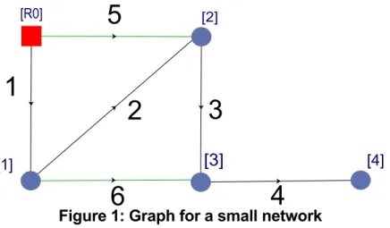
1.1. The hydraulic model and representation of the distribution network To model a network which might contain thousands of kilometres of pipes requires the system to be simplified. The Navier-Stokes equations are used for incompressible Newtonian fluids. The flow is considered permanent, unidirectional and uniformly mixed at junctions. Figure 1 shows a small network for whose hydraulic system is to be solved. The network is represented by a graph

i.e., a set of nodes and links.

Figure 1: Graph for a small network

A tree covering all nodes can be applied, given the flowrates of chords, all flow is calculated simply by applying the first equation of the system [HQ] below, a law of energy head loss must be chosen from the usual laws (Darcy Lechapt, Colebrook). The node / link incidence matrix of the network above is as follows:

Spanning tree !! !_! = −1 1 0 0 0 −1 1 0 0 0 −1 1 0 0 0 −1 1 0 0 0 1 0 0 −1 −1 0 0 0 0 1

The following equations describe, for any instant, the hydraulic equilibrium of the system:

(HQ) !_!! + ! = 0_!" ℎ − !_! !!_!− !_!!!_! = 0_!" ℎ = ℎ(!, !) (linear) (linear) (non linear)

(7)

Where nu is the number of junction nodes with unknown head; np is the number of pipes; d is the nodal demands with conceived beforehand values; Q is the flowrate vector in pipes (links); Hu is the head at junction nodes with unknown head and Hf the head at junction nodes with known head (reservoir and tanks); h is the head loss in pipes that is a function of the flowrate Q and the roughness K.

The system (HQ) consists of steady state equations. It is solved iteratively for a fixed time step (Piller 1995, Rossman 2000). Then the level of the storage tanks is updated with the following mass balance equation:

(0)

!_! ! = 0 = !_! is given The differentiable equation is solved by a forward Euler.

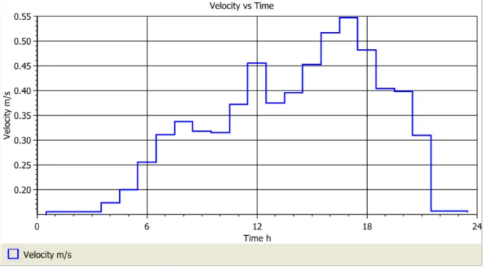
Outputs are piecewise constant flowrate and pressure function vs time. Illustration is given in Figure 2 for the velocity with an hourly timestep. The method is described as an "extended period simulation."

Figure 2: Piecewise constant Velocity vs time made with Porteau

1.2. Water quality model

The transport model uses hydraulic velocities as known variables and the advective transport and reaction are calculated. The determined variables can be the concentration of a monitored substance, the minimum, maximum or averaged by flowrates water age, or the tracking (provenance) of the sources. Generally, a relationship between the pipe and the kinetic product is used (kWall); it may be added to the kinetic product of the water (Kbulk).

The partial differential equation of the system, Eq (2), is solved with a timestep at most equal to the hydraulic one.

!!! !, ! + ! !, ! !!! !, ! + ! !, !, ! = 0 (2)

! 0, ! = !! ! , ! !, 0 = Φ ! , ∀ ! ≥ 0

(8)

The system is said to be weakly coupled.

The kinetic order (alpha) is any value greater or equal than one for any consideration of complex phenomena involving multiple interactions.

Reaction term: ! !, !, ! = !!! _{!, ! with α ≥ 1}

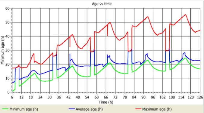
The calculation of the water age interval is illustrated in the Figure 3 below, with the minimum water age in green, the mean age in blue, and the maximum water in red.

Figure 3: Minimal, average and maximum age vs time made with Porteau software

The initial conditions (IC) are crucial because they may influence the results for several days. Usually zero values over the entire network is used, however it is necessary that sufficient time is calculated before any model prediction reflects reality. The graph in Figure 3 illustrates that 5 days of simulation are necessary to get stable water age results that are not influenced by the IC. For the concentration (Figure 4) 18h are needed to reach the observation node from the source and still 4 or 5 days are necessary to get the independence from the IC.

(9)

Figure 4: Concentration vs time with influence of initial condition made with Porteau

The coupling of hydraulic and quality systems is illustrated below, the parameters of the two systems (d, K) and (α, β) can be calibrated independently and the transport-reaction system solved independently of the hydraulic model solving.

Figure 5: Weak coupling between hydraulic and quality models

In summary, the results of hydraulic and transport models are piecewise constant values. The initial condition for the transport equation can strongly influence the results. Both models are weakly coupled: first we solve the hydraulic system and then the transport system.

(10)

2. Slow transient

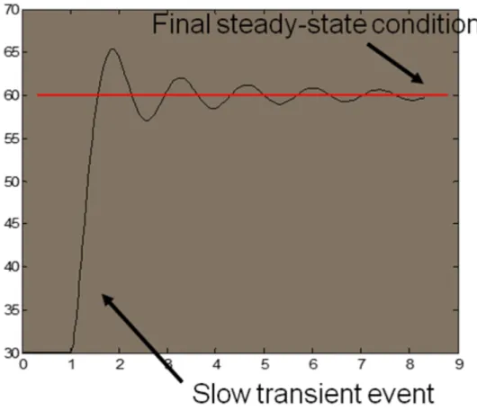
The above models have been designed for sizing optimization and off-line management. Their use online does not allow the reproduction of observations where the boundary conditions change continuously. For example, Figure 6 shows a slow transient event with a change of boundary condition which then remains constant for the observation. Consequently, the hydraulic state will vary continuously fairly fast before eventually stabilising and remaining constant.

In the real time Scada, the time step becomes very small and when the boundary conditions (tank, demand…) are changing and/or when control valves are acting, inertia terms have to be considered in the equations (Piller and Propato, 2006). Jaumouillé 2009, then Brémond et al. (2009) derived a slow transient pressure-driven model from Navier Stokes equations for incompressible flows to account for continuously time-varying velocity and leakage along pipes. As the velocities are continuously varying time functions, this impacts the water quality solving solution method (Fabrie et al., 2010).

Figure 6: Slow transient effect on a hydraulic variable

The hydraulic equations to be considered are:

!_!!_! = !_!(−ℎ ! + !_!!!_! ! + !_!!!_!(!) − !!_!(!)) !_!!_!= −!_!!

Where qc is the loop flow rate; the overdot is the time derivative; M0 is the loop-link incidence matrix; L is the link inertia rate; Lc = M0LM0T is the loop inertia rate; qd is the flow rate that corresponds to qc = 0; f refers to the free-surface tanks and r corresponds to the reservoir.

(11)

With ! = !! !! ! _{+ !} !; !! ! = −!!"## !! _{! !} 0_!!! !! 0 = !! !"# ℎ! 0 = ℎ!!(!")

These equations are solved with a time compatible with real-time execution. Irstea has a slow transient code that can be easily added to the Porteau software. 3S Consult also has a generic code that allows another form of slow transient calculation.

3. Diffusion and Dispersion

The diffusion is the process where a constituent moves from a higher concentration to a lower concentration. There are two kind of diffusion: the molecular diffusion for the fluid at rest and the eddy diffusion that corresponds to a turbulent mixing of particles to be considered in zones with large vortices. The dispersion is a mixing caused by the variation in velocities.

The advection-reaction transport models § 1.2 Eq. (2) show some approximations made as default for low velocities (case of transit by night or discharge pipes used during downtime). To improve this for transport in a pipe, it is necessary to take into account the molecular diffusion and dispersion. This builds on the work of (Lee, 2004) who showed the effect of diffusion on a contaminated liquid stream on a front at t = 0s, travelling first in the laminar regime for 2000s as shown in Figure 7, then stopped for 2000s to see the pollutant dispersion around the front cf. Figure 8.

Figure 7: Developing Phase with Advection Dispersion: D= 0.318 cm U= 0.4 cm/s and Re= 12.7

(12)

Figure 8: Relaxation Phase with Diffusion Only: D= 0.318 cm U= 0. cm/s and Re= 0.

A 1D Lagrangian advection-dispersion transport (LADT) is proposed improving efficiency vis-à-vis the dispersion. The adaptation of such a model using a Eulerian framework could be tested.

4. Mixing at junctions

The transport models that are currently used assume perfect mixing at junction nodes. Such a situation is not usually checked and depends on the network geometry and flow characteristics. Recent work at Sandia National Laboratories (2009) on this subject has led to the development of simple rules for the passage at a cross-junction directly applicable to the 1D model. This involves calculating the proportions of flows occurring in the mixture according to the different branches of the junction to infer imperfect mixing. Figure 9a illustrates the imperfect mixing of blue tracer dye. In the second case, Figure 9b, mixing is approximately perfect for both the north and west outlets.

Figure 9: Solute mixing in a pipe junction with adjacent inlets and unequal diameters (tracer inlet is on the right, clean inlet is at the bottom) Sandia 2009

(13)

Using a pilot site and 3D CFD modelling, the EPANET quality model (Rossman, 2000) was modified to best represent mixtures (Ho and O'Rear, 2009). This model is called BAM: Bulk advective Mixing. Figure 10 shows two situations where the greatest momentum is vertical (north) or horizontal (west). It is clear that in both situations a pollutant arriving with less momentum will not reach the outlets.

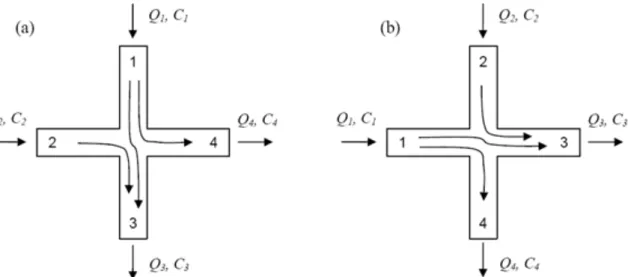
Figure 10: Description of the mixing variables at a cross by Sandia 2009, numbering assignment in the bulk mixing model for different flow configuration: a-the greatest

momentum is in the vertical; b-the greatest momentum is in the horizontal direction. Flow rate is denoted by Q [L3/T], and concentration is denoted by C

[M/L3]

For perfect mixing we have in the situation of Figure 10a and 10b, C3 and C4 output concentrations given by equation 3:

!_!"#$%&'& = !_! = !_! = !!!!!!!!!

!!!!! (3) This corresponds to an average of the input concentrations weighted by the flow rates.

(14)

The BAM model (Eq. 4) provides the weighting formula for inlet concentrations for the concentration of the outlet facing the greatest bulk fluid momentum:

!_! = !_!"# = !!!!! !!!!! !!

!! (4)

Then for the second outlet Eq. 5:

(5)

The last two equations correspond to the situation of Figure 10. However, they neglect several effects such as turbulent (eddy) diffusivity and instabilities at the impinging interface that appear when we consider the equations in 3D. Also, the situation is more an intermediate situation between the perfect mixing and BAM mixing. Therefore the following equation (Eq. 6) is proposed:

!_!"#$%&'( = !_!"# + ! !_!"#$%&'&− !_!"# (6)

With 0 ≤ ! ≤ 1.

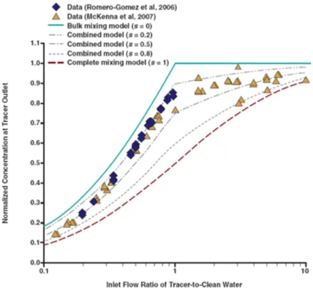
Equation 6 has been validated for different values of s by experimentation as illustrated in Figure (11) below.

Figure 11: Results of BAM model: Measured and predicted normalized concentrations at tracer outlet for different inlet flow rates and equal flow rates

However, with preliminary tests with CFD performed by Irstea using Ansys (2009) simple configurations with T-junction in series show Eq. 6 is not directly applicable and Eq. 3 is no

(15)

longer valid. Finding a 1D mixing law when two T-junctions are close to each other will be crucial to the project, particularly when one considers the large number of T-junctions compared to cross junctions for the SMaRT-OnlineWDN test case networks. Initial tests show that simplifications will be needed for application in the 1D model to represent various configurations of T-junctions in series leading to mixing laws approaching those for cross junctions but distinct depending on configurations and "inter- T-junction" distances, as shown in Figure 12.

Figure 12: Illustration of T junctions in a network

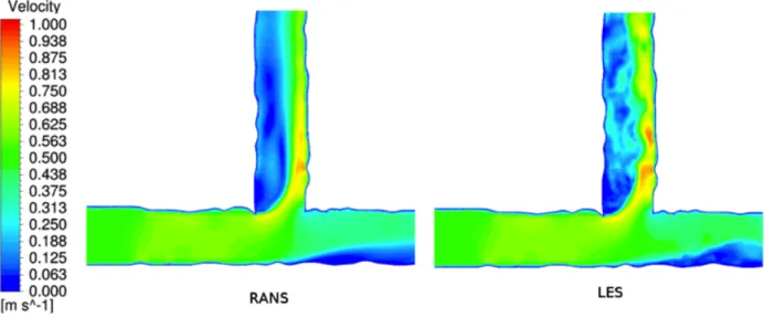
Modelling (Irstea and IOSB) and equivalent tests in the laboratory (TZW) will carefully analyse whether simplifications comparable with the EPANET BAM model may apply. 3D turbulent models are required to use a solving of type LES as RANS does not provide sufficient detail for medium scale turbulence and leads to strong approximations of the current lines and therefore on mixtures cf Figure 13.

Figure 13: 3D simulation with two models of turbulence RANS and LES

5. Roughness, diameter reduction and sedimentation

The following graph, Figure 14, shows a result for a mixture of two products of the same density; gravity has no effect. However, corrosion and hard fouling of the pipe also lead to significant deformation of streamlines and mixtures.

(16)

Figure 14: Fraction volume of two phases with the same velocity and density

The level of corrosion and fouling for a pipe is measured by equivalent sand roughness that is only known for new pipes. The roughness needs to be calibrated for aged pipes. The pipe diameter may also be reduced significantly and play a significant role in the residence time of the system. Christensen (2009) made a comparison with calibration of roughness with or without pipe diameters at the same extend. He reported better prediction for velocities, residence times, product kinetics and residual concentration of disinfectants. The influence of diameter on water age prediction and roughness estimation is shown in Figure 15.

Figure 15: Influence of diameter calibration on Water Age predictions

To show the effects of corrosion on the flows we did some tests on 3D CFD straight pipes and connections T-junctions. The effects on the current lines are clearly visible; the velocity profile Figure 16 is not formed as a smooth pipe, but more or less follows the previous deformation of the wall. The same is seen above in Figure 13, the mixing is strongly disrupted.

(17)

Figure 16: Velocity - longitudinal section and output; Uniform Velocity Inlet: 0.8 m/s (Re= 80000)

Given the difficulty of obtaining a profile of pipe wall fouling (3D laser) and the difficulty to simulate such behavior (fine mesh, LES), the simulations will focus primarily on smooth pipes and their joints (T-junction, multi T-junction).

For the SMaRT-OnlineWDN project, regular (annual) calibration of the equivalent roughness and diameter of the pipe is proposed rather than to model precisely the processes of sedimentation and corrosion.

6. Mixing in tanks

Mixing in storage tanks will also be improved as required in existing tools (Porteau, Sir) by the tested compartment models (LIFO, FIFO ...). However, the elaboration of a new model does not seem necessary for our purposes, because there will always be measures of tank inputs and outputs. Modelling the tank becomes a boundary condition. Tested EPANET models (Sandia 2009) already provide accuracy compatible with the measurements.

7. Multispecies and pathogens modelling

In the SMaRT-OnlineWFN_{project it is intended to model in real-time the hydraulic state and the} transport of the usual quality parameters such as chlorine concentration, residence time, tracking of the source, temperature and conductivity. The modelling of multi species and pathogens is out of the scope of the project. Moreover, a result from the SecurEau project (EU project n° 217976 under the call FP7-SEC-2007-1 is that non-specific water quality sensors may detect a chemical or biological contamination. This reinforces the need to model non-specific but classical water quality parameters online and not pathogens and multispecies.

8. Decision

(18)

Tableau 1: list of phenomena that will be developed Phenomena Will be developed

Slow transient yes

Cross and Tee junctions yes

Dispersion and diffusion yes

Pathogens no

Behaviour of multi-species no

Mixing in tanks no

Sedimentation no

Surface roughness yes

Diameters reduction yes

Modelling of one chemical

substance yes

9. Referred bibliography

Ansys Fluent 12.0 (2009), Theory guide.

Brémond, B., Fabrie, P., Jaumouillé, E., Mortazavi, I., and Piller, O. (2009). "Numerical simulation of a hydraulic Saint-Venant type model with pressure-dependent leakage." Applied Mathematics Letters, 22, 1694-1699.

Christensen Ryan T. (2009), Age effects on iron-based pipes in water distribution systems, Ph.D. thesis, Utah State University.

Fabrie, P., Gancel, G., Mortazavi, I., and Piller, O. (2010). "Quality Modeling of Water

Distribution Systems using Sensitivity Equations." Journal of Hydraulic Engineering, 136(1), 34-44.

C. Ho and L. O'Rear, Jr., (2009) “Evaluation of solute mixing in water distribution pipe junctions," American Water Works Association AWWA, vol. 101:9, pp. 116-127

Jaumouillé, E. (2009). "Contrôle de l'état hydraulique dans un réseau potable pour limiter les pertes," Applied Mathematics thesis from the University of Bordeaux, 132 pages, Talence, France.

Lee Y. (2004), Mass dispersion in intermittent laminar flow, Ph.D. thesis, Iowa State University, 2004.

Piller O. (1995), Modélisation du Fonctionnement d’un Reseau - Analyse hydraulique et choix de mesures pour l’estimationn des paramètres. PhD thesis, Université de Bordeaux I.

Piller, O., and Propato, M. (2006). "Slow Transient Pressure Driven Modeling in Water

Distribution Networks." 8th annual Water Distribution System Analysis Symposium, University of Cincinnatti, Cincinnati, Ohio USA, August 27-30 2006, printed by ASCE, 13.

Rossman L.A. (2000), EPANET 2 User Manual, National Risk Management Research Laboratory.

Sandia (2009), Joint Physical and Numerical Modeling of Water Distribution Networks, Internal report 130 pages.