Data analysis for stress measurements by overcoring : new optimization techniques
Texte intégral
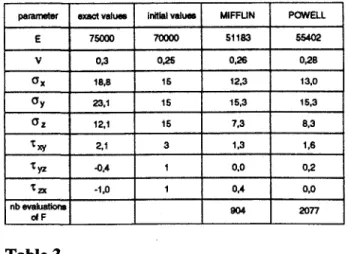
Figure
Documents relatifs
This algorithm is important for injectivity problems and identifiability analysis of parametric models as illustrated in the following. To our knowledge, it does not exist any
2. b) Derive the least squares solution of the unknown parameters and their variance-covariance matrix.. Given the angle measurements at a station along with their standard
In addition to its main goal, the experiment is well suited to determine the neutrino velocity with high accuracy through the measurement of the time of
The virtual gauge which corresponds to the positional tolerance is composed by a fitter 1 external cylinder (reference on the external surface) and five limitter internal cylinders..
The delays in producing the Target Tracker signal including the scintillator response, the propagation of the signals in the WLS fibres, the transit time of the photomultiplier
The special case of linear dynamical system with one-dimensional output the state of which is observed only on a short-time interval is consid- ered and it is shown that
In the last years, we have undertaken a comprehensive study of excited state lifetimes of single protonated aromatic amino acids and small peptides by means of femtosecond
In this paper, we demonstrate new state preparation and state detection techniques using 174 YbF molecules, which increase the statistical sensitivity to the eEDM by a factor of 20
